


ABSTRACT
Sex differences in birth weight contribute to within-litter variability, which itself is connected to piglet survival. Therefore, we studied whether the sex difference in piglet birth weight is a genetically variable sex dimorphism. For that purpose a linear mixed model including sex-specific additive genetic effects was set up. A hypothesis testing problem was defined to detect whether these genetic effects significantly differ between sexes. In a second step, the effect of sex-linked genes was studied explicitly by partitioning the additive genetic effects into autosomal and gonosomal effects. Furthermore, a definition of heritability for the sex difference of a randomly chosen pair of littermates with opposite sex was given. The proposed models were applied separately to a Landrace and Large White data set. Significant genetic variability for the sex dimorphism was found in Landrace (P = 0.03) but not in Large White (P = 0.10). Heritability estimates were at 3 to 5% depending on the model. The X-chromosomal genetic variation was not significant (P > 0.18) at all, whereas the Y-chromosome significantly (P < 0.01) contributed to the genetic variation in Landrace with a corresponding SD of 34 g. It can be concluded that the sex dimorphism of piglet birth weight is genetically variable and a potential target of genetic improvement.
INTRODUCTION
Sexually dimorphic trait expression appears in many species. For example, sex-linked genes are responsible for differences in wing, thorax, and head traits in Drosophila melanogaster (Cowley et al., 1986; Cowley and Atchley, 1988). The sex-specific abdominal pigmentation in D. melanogaster is due to a dimorphic expression of the genes at the Bab locus (Kopp et al., 2000; Couderc et al., 2002; Williams et al., 2008). Gene expression of the Bab locus is weaker in male abdomen than in females (Kopp et al., 2000). Kopp et al. (2003) applied QTL mapping techniques and identified the Bab locus as candidate gene. It caused 59% of the variation in female abdominal pigmentation in a panel of recombinant inbred lines of D. melanogaster. In a later work, Cowley et al. (1989) analyzed postnatal growth in mice. The authors reported that BW was sexually dimorphic at nearly every stage of age. In humans, Weiss et al. (2006) detected a wide range of sexually dimorphic traits (e.g., adult height, high-density lipoprotein cholesterol), but additive genetic variation that differed between males and females was found only for 2 traits (low-density lipoprotein cholesterol, lymphocyte count).
To identify genetic variation in traits of D. melanogaster, Cowley et al. (1986) included the effect of sex-linked genes by partitioning the additive genetic effect into autosomal and X-chromosomal effects. The authors were able to show that X-chromosomal variance exists for most wing length traits. The X-linked variance of males was twice the X-linked variance of females. The heritability of the difference in trait expression per sex was quite low (e.g., 4 to 7%) for the traits of wing length. The Y-chromosome was supposed to be highly heterochromatic in D. melanogaster, and hence its contribution to genetic variability was neglected in that study.
In pigs, birth weight is sex-specifically expressed. As an example, Arango et al. (2006) reported that male piglets were about 4% (about 55 g) heavier at birth than females. This sex difference contributes to the within-litter variability of birth weight (Wittenburg et al., 2008). Because the uniformity of birth weight is an important factor for piglet survival (English and Smith, 1995) or meat quality (Rehfeldt et al., 2008), breeding to reduce birth weight variability is of interest and has been previously determined to genetically affect growth and survivability (e.g., Högberg and Rydhmer, 2000; Damgaard et al., 2003).
In this paper we studied whether the sex difference in piglet birth weight is genetically variable. We fitted a linear mixed model (LMM) to birth weight and defined a hypothesis testing problem to detect whether the genetic effects significantly differ between sexes. In a second approach we studied the effect of sex-linked genes explicitly and applied a pedigree approach proposed by Fairbairn and Roff (2006). Additional to a fixed sex effect, we allow for variation caused by X-chromosomal loci as well as Y-chromosomal loci. Concerning this, the additive genetic effect was partitioned into autosomal and gonosomal effects. We set up a relationship matrix accounting for the X-chromosomal inheritance. The Y-chromosomal effect was traced back to the male founder animals. The proposed tools were applied to practical data sets of Landrace and Large White pigs.
MATERIALS AND METHODS
Animal Care and Use Committee approval was not obtained for this study because the data were obtained from an existing database of a commercial breeding organization.
Data
The data set was provided by the German breeding organization Bundeshybridzuchtprogramm. It consisted in total of 90,791 birth weights of Landrace (line LR, n = 45,172 piglets) and Large White pigs (line LW, n = 45,619 piglets) born within a period from January 2002 to August 2006. Sows were mated to 557 boars (line LR: 257; line LW: 300). Purebred litters of 3,637 sows (line LR: 1,968; line LW: 1,669) were observed. Only piglets born alive and sexed were weighed and included for further investigations. Most births were observed up to the third parity (41.1, 27.3, and 16.5%). The average birth weight of male piglets in line LR (line LW) was 1,677.10 g (1,529.63 g) with an SD of 364.42 g (356.27 g). Female piglets of line LR (line LW) had an average birth weight of 1,632.07 g (1,484.78 g) and the SD was 358.01 g (345.55 g). Hence, males were heavier but more variable in birth weight than females. The corresponding pedigree included 128,879 animals (line LR: Np = 64,943; line LW: Np = 63,936, with Np denoting the pedigree size) of up to 11 generations backward. The data were collected from 5 farms, where 3 farms bred sow line LR and 2 farms bred sow line LW exclusively. The following analyses were carried out separately for both pig lines.
The trait studied was the difference of male and female birth weight, which is a secondary trait. The primary observed phenotype is piglet birth weight itself. Because it is not straightforward to define a measure for the sex difference, we first fit a model to the primary trait. Afterward the genetic components are evaluated and derived for the secondary trait.
Model 1: Additive Genetic Effect Differing Between Sexes
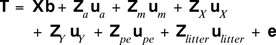
It was studied whether the difference in birth weight of male and female piglets is partly under genetic control. Bold symbols are used for vectors and matrices. We set up the following LMM for the vector of piglet birth weights, T, which included, among others, a fixed sex effect and an additive genetic component differing between sexes. It is
The vector of fixed effects  summarizes the effects of farm-year-season bf (line LR: 53; line LW: 38 levels), parity of sow bpa (1, 2, 3, ≥4), and sex bg (g = 1, 2 for males and females). The random effects are normally distributed, where
  describes the direct genetic effects of male and female piglets. The um indicates the maternal genetic effect. The covariance matrix of the genetic effects will be specified below. Furthermore,
  with I denoting the identity matrix of appropriate size, reflects the permanent environment affecting all offspring of 1 sow, and
  denotes the permanent environment within 1 litter. The residual deviation is normally distributed with
  The X and Zk denote the design matrices for the fixed effects and the random effects
  respectively. Note that Za is an
  matrix with
  where incidence is made in that submatrix corresponding to the sex of the piglet.
It is assumed that the genetic effects differ among male and female offspring. Furthermore, the correlation between the genetic effects ua and um has to be considered. With use of the (Np × Np) numerator relationship matrix A, it is assumed that
The covariance matrix of the direct genetic effects is  The genetic correlation
  is included in
  It has to be tested whether the genetic variation is the same for males and females, meaning
 Thus, the absence of any sex effect on the genetic components implies the null hypothesis,
and its alternative is HA: Σ is positive definite. Note that the null model equals a typical single-trait animal model. Under H0, where the breeding values are identical, the parameter  is located at the boundary of its parameter space [−1,1] and the variance component
  is unknown but equal to
  This testing problem can be examined by a likelihood ratio test. The corresponding test statistic is the restricted likelihood ratio test statistic (RLRT), which is twice the difference of restricted normal log-likelihood functions of the full model [M1] and the respective model under H0 in Eq. [2]. For independently distributed response variables, Self and Liang (1987) derived the asymptotic null distribution of RLRT as a 50:50 mixture of χ2 distributions with 1 and 2 df
Because the required regularity assumption of independence may be violated (e.g., due to the relationship structure in A), the asymptotic result of the RLRT null distribution should be applied with care.
Once significance of the genetic difference in birth weight per sex has been proved, a measure of heritability is required. For that purpose we construct an artificial trait describing the sex difference in birth weight. Assuming that both sexes appear in a litter, we define this trait by the difference in male birth weight (T1) and female birth weight (T2) of a randomly chosen pair of littermates and set
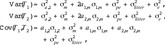
In view of model [M1] and under the assumption that no inbreeding appears, the variance and covariance of T1 and T2 and are given by
where 
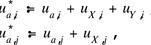
 and
and  are entries of the relationship matrix A. Because littermates are full sibs, it is
  For unrelated parents (as in the base generation), the coefficient of relation between mother and offspring is
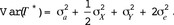
  Hence the total phenotypic variance of
  is
is
The genetic variability due to the difference in genetic effects is 

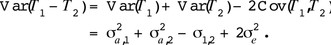
The heritability of the artificial trait  is defined as the proportion of genetic variability to the phenotypic variance of
Model 2: Autosomal and Gonosomal Effects
To identify the origin of sex-specific variation in birth weight, we may distinguish between autosomal and gonosomal inheritance. If only X-chromosomal inheritance would be considered (as suggested by Fairbairn and Roff, 2006), then it was suspected that variation in female birth weight was larger than in males. The raw SD of birth weights for this data set disagreed with that assumption. Hence Y-chromosomal inheritance was also included. Now we studied the autosomal genetic effects (not differing between sexes) and introduced additional vectors uX and uY accounting for the X-chromosomal and Y-chromosomal effects, respectively. We define the following LMM for piglet birth weight
The effects b, um, upe, ulitter, and e coincide with model [M1]. The autosomal genetic effect ua and maternal effect um may have a joint normal distribution
It is assumed that  where the
  covariance matrix S describes the relationship between individuals in terms of the X-chromosomal loci. The matrix S is set up as in Fernando and Grossman (1990) using gametic inbreeding coefficients (Wang et al., 1995). For male i, it is valid that
  and for a non-inbred female j, it is
  Furthermore, it is
  where the number of levels of uY is equal to the number of male founder animals.
Now the presence of sex-specific variation in birth weight is tested. Omitting the gonosomal effects, we start with the null model [M1], where the condition in Eq. [6] holds (i.e., the animal model). As a first step, we include the Y-chromosomal effect uY. The restricted likelihood ratio test is applied to the testing problem

If significance is proved, then the X-chromosomal effect uX is added and yields model [M2]. Otherwise, in case of nonsignificance, the X-chromosomal effect is added to the null model. We test for the variance component  Both testing problems have in common that the variance component in question lies at the boundary of its parameter space
  under H0. Then the null distribution of the test statistic RLRT may be roughly approximated by a 50:50 mixture of χ2 distributions with 0 and 1 df (Self and Liang, 1987).
We studied a measure of heritability for the difference in birth weight  in Eq. [4], which is obtained similarly to the function in Eq. [5]. Assuming no inbreeding, the phenotypic variance of
  is given by
If the breeding values of male i and female j are defined as
then the genetic variability due to the difference in breeding values is
Eventually, the heritability is obtained as
Model 3: Combined Model
Looking back on the sexually dimorphic impact of the Bab locus on abdominal pigmentation in D. melanogaster, one may think about possible interactions between autosomes and gonosomes. The Bab locus is situated on the third chromosome, which is an autosome (Kopp et al., 2000). To include such interactions in the study of piglet birth weight, we combined the approaches presented above. The third model (called [M3]) includes the effect of autosomes, which is different for males and females, and the effect of gonosomes. This approach is identical to model [M2] but with the condition in Eq. [1] fulfilled.
Software
The estimation and prediction of fixed and random effects, respectively, and the REML estimation of variance components were carried out with ASReml 2.0 (Gilmour et al., 2006). Using ASReml the significance of the fixed sex effect was tested by an F-test with adjusted denominator degrees of freedom (Kenward and Roger, 1997). In the study of X-chromosomal effects the gametic inbreeding coefficients were calculated with subroutines of the Fortran program package COBRA (Baes and Reinsch, 2007).
RESULTS
The analysis of piglet birth weight per model [M1] confirmed that the fixed sex effect  on birth weight was significantly present (P < 0.001). Male piglets were on average 49.76 g (47.34 g) heavier than females at birth in line LR (line LW). The estimated variance components are listed in Table 1. As an example for pig line LR, the estimated phenotypic SD in males was 361.16 g and in females 357.91 g. Most of the variation was caused by dam-related sources. In LR pigs, 14.89% of the phenotypic variation of males was due to maternal genetic effects. Furthermore, permanent environmental effects accounted for 4.40% and the permanent environment within litter contributed 19.00% to the phenotypic variation of males. In both pig lines, inbreeding was in average 2% on the level of litter.
Estimated variance components and SE (in parentheses) based on model [M1] including direct genetic effects for males and females1
| Component | Line LR | Line LW |
|---|---|---|
 | 7,531.95 (1,900.02) | 5,144.59 (1,618.94) |
 | 6,233.84 (1,671.82) | 4,436.09 (1,460.23) |
 | 5,599.43 (1,646.05) | 4,290.21 (1,478.12) |
 | −5,081.02 (2,034.33) | −1,368.10 (1,912.93) |
 | −5,489.75 (1,870.75) | −2,370.97 (1,845.63) |
 | 19,420.50 (2,932.17) | 18,549.20 (3,025.87) |
 | 5,739.94 (1,565.56) | 5,924.92 (1,680.64) |
 | 24,788.40 (984.79) | 25,087.80 (933.40) |
 | 78,038.90 (1,000.72) | 68,619.40 (874.92) |
| h2 | 4.23 (1.05) | 3.51 (1.05) |
| Component | Line LR | Line LW |
|---|---|---|
| 7,531.95 (1,900.02) | 5,144.59 (1,618.94) |
| 6,233.84 (1,671.82) | 4,436.09 (1,460.23) |
| 5,599.43 (1,646.05) | 4,290.21 (1,478.12) |
| −5,081.02 (2,034.33) | −1,368.10 (1,912.93) |
| −5,489.75 (1,870.75) | −2,370.97 (1,845.63) |
| 19,420.50 (2,932.17) | 18,549.20 (3,025.87) |
| 5,739.94 (1,565.56) | 5,924.92 (1,680.64) |
| 24,788.40 (984.79) | 25,087.80 (933.40) |
| 78,038.90 (1,000.72) | 68,619.40 (874.92) |
| h2 | 4.23 (1.05) | 3.51 (1.05) |
1 and
and  = variance of direct genetic effects of males and females, respectively, and the covariance
  between those;
  = variance of maternal effect and covariance
 between maternal effect and male (female) breeding value;
  = variance of permanent environmental effect;
  = variance of environmental effect within litter;
  = residual variance; h2 = heritability of sex difference × 100; LR = Landrace; LW = Large White.
Estimated variance components and SE (in parentheses) based on model [M1] including direct genetic effects for males and females1
| Component | Line LR | Line LW |
|---|---|---|
| 7,531.95 (1,900.02) | 5,144.59 (1,618.94) |
| 6,233.84 (1,671.82) | 4,436.09 (1,460.23) |
| 5,599.43 (1,646.05) | 4,290.21 (1,478.12) |
| −5,081.02 (2,034.33) | −1,368.10 (1,912.93) |
| −5,489.75 (1,870.75) | −2,370.97 (1,845.63) |
| 19,420.50 (2,932.17) | 18,549.20 (3,025.87) |
| 5,739.94 (1,565.56) | 5,924.92 (1,680.64) |
| 24,788.40 (984.79) | 25,087.80 (933.40) |
| 78,038.90 (1,000.72) | 68,619.40 (874.92) |
| h2 | 4.23 (1.05) | 3.51 (1.05) |
1 and = variance of direct genetic effects of males and females, respectively, and the covariance between those; = variance of maternal effect and covariance between maternal effect and male (female) breeding value; = variance of permanent environmental effect; = variance of environmental effect within litter; = residual variance; h2 = heritability of sex difference × 100; LR = Landrace; LW = Large White.
The analysis of model [M1] revealed that the correlation  between the direct genetic effects of males and females was close to 1 in both lines (line LR: 0.96, line LW: 0.94). For the significance test with regard to the question whether genetic effects differ between sexes in line LR, the test statistic was observed as 6.06, whereas in line LW it was 3.82. In line LR, the birth weight showed additive genetic variability differing between sexes (P = 0.031). Genetic evidence for the difference in birth weight per sex could not be excluded clearly for line LW (P = 0.099). In line LR, the heritability for the difference in birth weight was estimated as
  (line LW:
  Note that on the basis of model [M1], birth weights of males and females were defined as 2 distinct traits. If heritability was determined for these primary traits, then its estimates were
  for birth weight of males and
  for females in line LR
 in line LW).
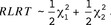
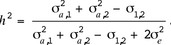
The study of gonosomal effects per model [M2] led to the estimates of variance components listed in Table 2. Birth weights of males separated by the Y-chromosomal inheritance were less variable in LW pigs than in LR pigs (Figure 1). The Y-chromosome was traced back to 30 founders in line LR, and 17 founders were identified in line LW. Testing for gonosomal effects showed that the Y-chromosomal effect was significantly present in pig line LR (P = 0.004) but not in LW (P = 0.444). Furthermore, the X-chromosomal inheritance can be neglected. Its variance component did not differ significantly from 0 in both lines (LR: P = 0.183, LW: P = 0.312). Hence, loci situated on the Y-chromosome caused more variation in birth weight than X-chromosomal loci. The estimates of heritability for the difference in birth weight were quite similar to the results above (i.e.,  in line LR and
  in line LW). Again, the fixed sex effect was significantly different from 0 in both lines (P < 0.001).
Estimated variance components and SE (in parentheses) based on model [M2] including autosomal and gonosomal effects1
| Component | Line LR | Line LW |
|---|---|---|
 | 5,767.13 (1,600.71) | 4,435.23 (1,444.10) |
 | −5,127.56 (1,862.79) | −2,560.74 (1,859.24) |
 | 19,613.10 (2,927.70) | 19,071.10 (3,077.90) |
 | 177.25 (237.38) | 111.21 (228.74) |
 | 1,182.54 (685.35) | 1.70 (28.35) |
 | 5,622.46 (1,563.83) | 6,039.29 (1,689.31) |
 | 24,748.40 (982.73) | 25,095.20 (933.75) |
 | 78,399.30 (965.46) | 68,784.50 (864.84) |
| h2 | 4.30 (1.05) | 3.16 (1.02) |
| Component | Line LR | Line LW |
|---|---|---|
| 5,767.13 (1,600.71) | 4,435.23 (1,444.10) |
| −5,127.56 (1,862.79) | −2,560.74 (1,859.24) |
| 19,613.10 (2,927.70) | 19,071.10 (3,077.90) |
| 177.25 (237.38) | 111.21 (228.74) |
| 1,182.54 (685.35) | 1.70 (28.35) |
| 5,622.46 (1,563.83) | 6,039.29 (1,689.31) |
| 24,748.40 (982.73) | 25,095.20 (933.75) |
| 78,399.30 (965.46) | 68,784.50 (864.84) |
| h2 | 4.30 (1.05) | 3.16 (1.02) |
1 = variance of autosomal effect;
  = variance of maternal effect and the covariance
  between both;
  and
and  = variance of X- and Y-chromosomal effect, respectively;
  = variance of permanent environmental effect;
  = variance of environmental effect within litter;
  = residual variance; h2 = heritability of sex difference × 100; LR = Landrace; LW = Large White.
Estimated variance components and SE (in parentheses) based on model [M2] including autosomal and gonosomal effects1
| Component | Line LR | Line LW |
|---|---|---|
| 5,767.13 (1,600.71) | 4,435.23 (1,444.10) |
| −5,127.56 (1,862.79) | −2,560.74 (1,859.24) |
| 19,613.10 (2,927.70) | 19,071.10 (3,077.90) |
| 177.25 (237.38) | 111.21 (228.74) |
| 1,182.54 (685.35) | 1.70 (28.35) |
| 5,622.46 (1,563.83) | 6,039.29 (1,689.31) |
| 24,748.40 (982.73) | 25,095.20 (933.75) |
| 78,399.30 (965.46) | 68,784.50 (864.84) |
| h2 | 4.30 (1.05) | 3.16 (1.02) |
1 = variance of autosomal effect; = variance of maternal effect and the covariance between both; and = variance of X- and Y-chromosomal effect, respectively; = variance of permanent environmental effect; = variance of environmental effect within litter; = residual variance; h2 = heritability of sex difference × 100; LR = Landrace; LW = Large White.
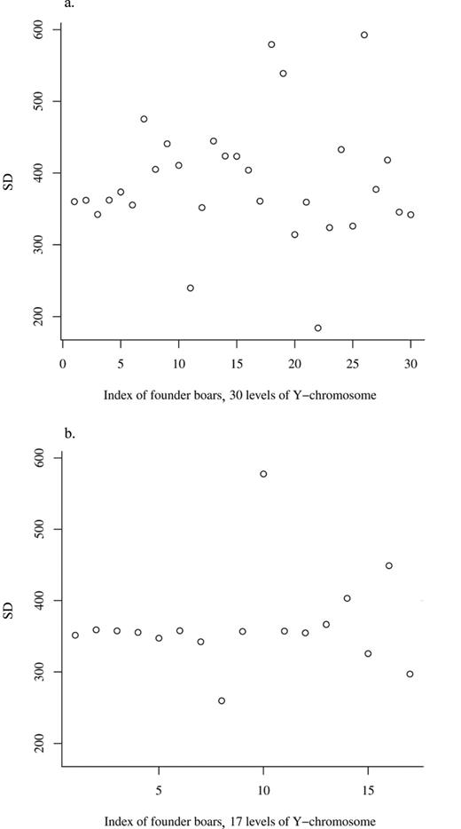
Sample SD of birth weights of males separated by the Y-chromosome of founders: a) Landrace and b) Large White pigs.
Last, results for the combined model [M3] are presented in Table 3. The estimates of heritability increased slightly to 4.81 and 3.50% in line LR and LW, respectively. The autosomal effects of males and females were rather similar to the additive genetic effects per sex of the first approach (model [M1]), whereas the variation of gonosomal effects changed. The Y-chromosomal effect was still significantly present (P = 0.014) in LR. In line LW, neither the X-chromosomal effect nor the Y-chromosomal effect was significant.
Estimated variance components and SE (in parentheses) based on model [M3] including direct genetic effects for males and females and gonosomal effects1
| Component | Line LR | Line LW |
|---|---|---|
 | 7,763.90 (54.80) | 5,129.19 (1,617.70) |
 | 6,357.91 (44.88) | 4,427.59 (1,461.09) |
 | 5,356.58 (37.81) | 4,241.86 (1,503.29) |
 | −5,555.59 (39.21) | −1,390.60 (1,913.96) |
 | −5,924.43 (41.82) | −2,392.43 (1,847.79) |
 | 21,143.90 (149.24) | 18,563.40 (3,027.63) |
 | 228.58 (237.19) | 55.99 (269.19) |
 | 1,005.56 (643.76) | 0.01 (0.00) |
 | 5,093.96 (1,106.54) | 5,925.58 (1,680.86) |
 | 24,732.20 (976.09) | 25,086.80 (933.41) |
 | 77,925.00 (550.01) | 68,620.70 (874.72) |
| h2 | 4.81 (0.38) | 3.50 (1.05) |
| Component | Line LR | Line LW |
|---|---|---|
| 7,763.90 (54.80) | 5,129.19 (1,617.70) |
| 6,357.91 (44.88) | 4,427.59 (1,461.09) |
| 5,356.58 (37.81) | 4,241.86 (1,503.29) |
| −5,555.59 (39.21) | −1,390.60 (1,913.96) |
| −5,924.43 (41.82) | −2,392.43 (1,847.79) |
| 21,143.90 (149.24) | 18,563.40 (3,027.63) |
| 228.58 (237.19) | 55.99 (269.19) |
| 1,005.56 (643.76) | 0.01 (0.00) |
| 5,093.96 (1,106.54) | 5,925.58 (1,680.86) |
| 24,732.20 (976.09) | 25,086.80 (933.41) |
| 77,925.00 (550.01) | 68,620.70 (874.72) |
| h2 | 4.81 (0.38) | 3.50 (1.05) |
1 and
and  = variance of direct genetic effects of males and females, respectively, and the covariance
  between those;
  = variance of maternal effect and covariance
 between maternal effect and male (female) breeding value;
  and
and  = variance of X- and Y-chromosomal effect, respectively;
  = variance of permanent environmental effect,
  = variance of environmental effect within litter;
  = residual variance; h2 = heritability of sex difference × 100; LR = Landrace; LW = Large White.
Estimated variance components and SE (in parentheses) based on model [M3] including direct genetic effects for males and females and gonosomal effects1
| Component | Line LR | Line LW |
|---|---|---|
| 7,763.90 (54.80) | 5,129.19 (1,617.70) |
| 6,357.91 (44.88) | 4,427.59 (1,461.09) |
| 5,356.58 (37.81) | 4,241.86 (1,503.29) |
| −5,555.59 (39.21) | −1,390.60 (1,913.96) |
| −5,924.43 (41.82) | −2,392.43 (1,847.79) |
| 21,143.90 (149.24) | 18,563.40 (3,027.63) |
| 228.58 (237.19) | 55.99 (269.19) |
| 1,005.56 (643.76) | 0.01 (0.00) |
| 5,093.96 (1,106.54) | 5,925.58 (1,680.86) |
| 24,732.20 (976.09) | 25,086.80 (933.41) |
| 77,925.00 (550.01) | 68,620.70 (874.72) |
| h2 | 4.81 (0.38) | 3.50 (1.05) |
1 and = variance of direct genetic effects of males and females, respectively, and the covariance between those; = variance of maternal effect and covariance between maternal effect and male (female) breeding value; and = variance of X- and Y-chromosomal effect, respectively; = variance of permanent environmental effect, = variance of environmental effect within litter; = residual variance; h2 = heritability of sex difference × 100; LR = Landrace; LW = Large White.
DISCUSSION
Genetic Variation Differing Between Sexes
We have shown that the sex difference in piglet birth weight is genetically variable, at least in 1 pig line. The first approach (model [M1]) was carried out to identify whether the genetic effects differ between sexes. The second approach (model [M2]), which includes the effects of X- and Y-chromosomal loci, was more suitable to study the origin of sex-specific trait variation. The latter approach was computationally more demanding. The inverse of the relationship matrix S, which accounts for the X-chromosomal inheritance, had to be determined in advance.
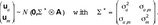
An alternative approach, which is similar to model [M1], leads to a reduced dimensionality of the analysis, because it applies only 1 breeding value  per individual i. Set
  with indicator variable
  if the ith individual is male and 0 otherwise. The w denotes a factor of proportionality between genetic variation of males and females. The vector of sexless genetic effects is
  with
with  We assume that the genetic variation differs between sexes
where  is the (i, j)th entry of the numerator relationship matrix A. In future studies, the variance component
  and the factor w may be estimated, for example, via REML. Additionally, one could test for
  vs.
vs. 
Model Extensions
The models [M1] or [M2] can be extended further if desired. Any random effect can be split into sex-specific components and a correlation between those. As an example, environmental effects may differ between males and females, and this fact is considered by the vector  which may have the joint distribution
Dam-related sources of variability (maternal genetic, permanent, and litter) are by far more important than direct genetic for the primary trait birth weight (e.g., also see Roehe, 1999). The possible question of their sex specificity was not further investigated, but would be a necessary condition for their contribution to variation of the sex difference. One may imagine differences in developmental stability of sexes in an interplay with variation in the ability of the dam to buffer disturbances. Though this could probably lead to sex-specific maternal variability, analyses were restricted to sex specificity of direct genetic effects, which were anticipated as the most likely source of variation for the difference.
The models presented in this paper are applicable to any continuous trait that is sex-specifically expressed. But also noncontinuous or categorical traits may be influenced by sex-linked regions. As an example, Knol et al. (2002) found that preweaning survival rates are larger in female piglets than in males. In those applications where discrete data have to be studied, the genetic effect differing between sexes should be included in a generalized linear mixed model with adequately chosen link function.
Heritability of Sex Difference
The derivation of heritability in Eq. [5] on the basis of 2 littermates is quite plain. Litter size and the proportion of sexes within litter may have an influence on the measure of heritability. In line LR, in average 5.4 male and 5.3 female piglets were born alive (5.7 males and 5.6 females in LW). Hence we have also determined heritability on the basis of total litter size. Let T1 and T2 be the average birth weights among males and females, respectively, within litter of size  The trait of interest is the difference of the average birth weight (i.e.,
  The calculation of its (co-) variance components is omitted for brevity (available from the authors). Eventually, the heritability is obtained as
Applying this formula to the variance components estimated via model [M1] yielded  in LR and
  in LW. In comparison to the estimates for a pair of piglets (Eq. [5]), a difference was only observed in LR. For larger differences between
  and
and  litter size has more impact on heritability.
Because the analyses made in this study are based on birth weight of liveborn piglets, the genetic parameters are potentially underestimated. In an earlier paper (Wittenburg et al., 2010) we studied the influence of including or not including birth weight of stillborns on the variation of birth weight within litter. Even though the genetic variance components were slightly underestimated with stillborns omitted, the estimates of heritability did not differ significantly if either birth weights of all piglets were involved or stillborns were omitted. It would be interesting to prove this hypothesis for individual birth weight, too. Birth weights of stillborns were not available in the underlying data sets.
Benefit in Future Selection
In all cases, the estimates of heritability for the sex difference in birth weight were in the same range (3 to 5%), which shows robustness of the methods presented and the possibility of genetic improvement. In newborn piglets, the sex difference is of special interest because it directly contributes to within-litter variability (Wittenburg et al., 2008). Minimizing the sex difference reduces the within-litter variance of birth weight and thereby has a positive impact, for example, on preweaning survival (Roehe and Kalm, 2000).
In later ages, heritabilities for sex differences in production traits are presumed to be even larger because effects of differential development between sexes accumulate with age. But for these traits having both sexes represented in performance testing, no matter whether it is a sire line or a dam line, may be sufficient to prevent undesirable genetic trends for sex differences. Unlike for birth weight, the importance of sex differences for production traits also depends on the practices applied by industry (e.g., split-sex finishing or finishing of entire males or castrates). In conclusion, the proposed models are well-suited for analyzing the genetics of a sex dimorphism and may also be applied by the pig industry to gain insight into the amount of genetic variation in specific populations, for monitoring genetic trends for sex differences, and for the sake of genetic improvement.
LITERATURE CITED
Footnotes
We thank Hubert Henne from the Bundeshybridzuchtprogramm (Züchtungszentrale Deutsches Hybridschwein GmbH, Dahlenburg-Ellringen, Germany) for providing the extensive data. We also thank the anonymous reviewers for their constructive comments. The research project was financially supported by the H. Wilhelm Schaumann Stiftung, Hamburg, Germany.
