


ABSTRACT
This study sought to assess whether residual feed intake (RFI) calculated by regressing feed intake (DMI) on growth rate (ADG) and metabolic mid-BW in 3 different ways led to similar estimates of genetic parameters and variance components for young growing cattle tested for feed intake in fall and winter seasons. A total of 378 beef steers in 5 cohorts were fed a typical high energy feedlot diet and had free-choice access to feed and water. Feed intake data were collected in fall or winter seasons. Climate data were obtained from the University of Alberta Kinsella meteorological station and Vikings AGCM station. Individual animal RFI was obtained by either fitting a regression model to each test group separately (RFIC), fitting a regression model to pooled data consisting of all cohorts but including test group as a fixed effect (RFIO), or fitting a regression to pooled data with test group as a fixed effect but within seasonal (fall-winter or winter-spring) groups (RFIS). Two animal models (M1 and M2) that differed by the inclusion of fixed effects of test group or season, respectively, were used to evaluate RFI measurements. Feed intake was correlated with air temperature, relative humidity, solar radiation, and wind speed (−0.26, 0.23, 0.30, −0.14 for fall-winter and 0.31, −0.04, 0.14, 0.16 for winter-spring, respectively), but the nature and magnitude of the correlations were different for the 2 seasons. Single trait direct heritability, model likelihood, direct genetic variance, and EBV accuracy estimates were greatest for RFIC and least for RFIO for both M1 and M2 models. A significant genetic correlation was also observed between RFIO and ADG, but not for RFIC and RFIS. Including a season effect (M2) in the genetic evaluation of RFIO resulted in the smallest heritability, model LogL, EBV accuracy, and largest residual variance estimates. These results, though not conclusive, suggest a possible effect of seasonality on feed intake and thus feed efficiency.
INTRODUCTION
Residual feed intake (RFI) is increasingly becoming the standard measure for evaluating feed efficiency. The trait is typically a linear function of feed intake, BW, and BW gain (Koch et al., 1963; Arthur et al., 2001) and any other measurable energy sinks (Crews, 2005), such as body composition and lactational performance (Veerkamp et al., 1995; Montanholi et al., 2009). The intention of having RFI net of correlated traits is such that differences in efficiency between animals are due to differences in metabolic efficiency rather than in production (Crews, 2005).
Variations in animal performance occasioned by seasonal changes in environmental and climatic conditions are known to occur (Birkelo et al., 1991). Such variations are thought to be due to differences in adaptation and efficiency of energy utilization in response to the requisite energy demands. The effects of ambient temperature on animal performance have also been widely studied in beef cattle. Exposure to extended periods of cold can lead to cold stress, invoking various thermoregulatory mechanisms such that maintenance requirements remain unchanged until a critical temperature is surpassed (Young, 1983). Metabolic acclimatization due to exposure to cold temperatures has been thought to reduce performance and efficiency in animals compared with those not exposed to such conditions at the same feed intake (Young, 1981). Residual feed intake measures individual animal differences in maintenance requirements after adjusting for growth. Consequently, due to the increased physiological demand in cold conditions, RFI estimated in winter periods may represent a different trait from that obtained in warmer seasons. This study sought to compare if there were significant differences in the performance and efficiency of groups of steers tested for feed intake in 2 periods (fall-winter and winter-spring seasons) over 3 successive years.
MATERIALS AND METHODS
All animals were cared for following the protocols and guidelines outlined by the Canadian Council on Animal Care (CCAC, 1993).
The data consisted of 378 beef steers, offspring of a cross between a composite dam line, (generated as an experimental dam population after 30 yr of selection) and Angus, Charolais, or University of Alberta hybrid bulls. The dams used were produced from crosses among 3 composite cattle lines, namely beef synthetic 1, beef synthetic 2, and dairy × beef synthetic. Beef synthetic 1 was composed of 33% Angus, 33% Charolais, and about 20% Galloway, among other beef breeds whereas beef synthetic 2 was composed of 60% Hereford with the remaining 40% being other beef breeds. The dairy × beef synthetic was composed of approximately 60% dairy breeds (Holstein, Brown Swiss, or Simmental) and 40% beef breeds, mostly Angus and Charolais (Goonewardene et al., 2003). Sire and breed distributions for fall-tested and winter-tested groups are shown in Table 1. Feed intake data were collected using the GrowSafe automated feeding system (GrowSafe Systems Ltd., Airdrie, Canada) over a period of 3 yr with 2 cohorts of animals tested for feed efficiency in each year, except in yr 1 where 1 cohort was included in the analysis (Table 1). Feeding behavior data (number of feeding events, feeding duration, and head-down time) were also collected from the GrowSafe system and summed to obtain daily counts following similar methods as those in Basarab et al. (2003).
Summary of the number of steers per sire, within test group and sire breed
| Item | Fall-winter | Winter-spring |
|---|---|---|
| Steers, No. per year | ||
| Year | ||
| 20031 | NA2 | 64 |
| 20043 | 80 | 76 |
| 20054 | 80 | 78 |
| Breed5 | ||
| Angus | 26, 44, 70 | 22, 45, 26, 93 |
| Charolais | 41, 12, 53 | 19, 14, 11, 44 |
| Hybrid | 13, 24, 37 | 23, 17, 41, 81 |
| Sires | ||
| Total No. of sires | 34 | 55 |
| Average No. of offspring per sire | 4.7 | 3.96 |
| No. of sires with single offspring | 19 | 38 |
| Average No. of offspring per sire6 | 9.4 | 10.59 |
1Number of steers for cohort 1 (fall-winter) and cohort 2 (winter-spring).
2NA = not analyzed.
3Number of steers for cohort 3 (fall-winter) and cohort 4 (winter-spring).
4Number of steers for cohort 5 (fall-winter) and cohort 6 (winter-spring).
5Number of steers for cohorts 3, 5, and total (fall-winter) and cohorts 2, 4, 6, and total (winter-spring).
6Average for sires with more than 1 offspring.
The test diets consisted of standard high energy feedlot diets as shown in Table 2 (Nkrumah et al., 2007). Each formulation of the test diet was sampled approximately once every 2 wk and composited monthly. The composite samples were mixed and subsampled for in vivo digestibility tests whereas the 3 pooled samples were analyzed as triplicates for proximate analysis to ascertain nutrient and DM content as described by Nkrumah et al. (2004, 2006). The nutrient compositions reported were averaged across the triplicates (Table 2). The testing periods lasted approximately 90 d, and animals had free-choice access to feed and drinking water. Body weight data were recorded every 2 wk, with the first BW obtained on the day preceding the test. The exception was for yr 1 where BW were recorded weekly. The last BW was obtained as close to the end of test as possible, generally within 2 to 3 d before the end of the experiment. Ultrasound backfat thickness, measured between the 12 and 13th rib, was obtained at the end of the feed intake test using an ultrasound transducer as described by Basarab et al. (2003).
Nutrient composition and ingredients of experimental diets for the years tested
| Item | 2003 | 2004 | 2005 |
|---|---|---|---|
| Ingredient, %, as-fed basis | |||
| Dry-rolled corn | 80.00 | — | — |
| Barley grain | — | 64.50 | 64.50 |
| Oat grain | — | 20.00 | 20.00 |
| Alfalfa hay | 13.50 | 9.00 | 9.00 |
| Beef feedlot supplement1 | 5.00 | 5.00 | 5.00 |
| Canola oil | 1.50 | 1.50 | 1.50 |
| DM, % | 90.50 | 88.90 | 88.90 |
| Nutrient composition, DM basis2 | |||
| ME, Mcal/kg | 2.90 | 2.91 | 2.91 |
| CP, % | 12.50 | 14.00 | 14.00 |
| Crude fat, % | — | — | — |
| NDF, % | 18.30 | 21.49 | 21.49 |
| ADF, % | 5.61 | 9.50 | 9.50 |
1Contained 440 mg/kg of monensin (Cargill Feeds, Camrose, Alberta, Canada), 5.5% Ca, 0.28% P, 0.64% K, 1.98% Na, 0.15% S, 0.31% Mg, 16 mg/kg of I, 28 mg/kg of Fe, 1.6 mg/kg of Se, 160 mg/kg of Cu, 432 mg/kg of Mn, 432 mg/kg of Zn, 4.2 mg/kg of Co, as well as a minimum of 80,000 IU/kg of vitamin A, 8,000 IU/kg of vitamin D, and 1,111 IU/kg of vitamin E.
2Obtained from digestibility trials and subsequent proximate analysis as described by Nkrumah et al. (2006).
Climate data (average, minimum and maximum air temperature, average relative humidity, average solar radiation, and wind speed) for the years 2003–2004 (designated year 2004) and 2004 to 2005 (2005) were obtained from the University of Alberta Kinsella meteorological station. The Kinsella station was installed in October 2003, such that data for 2002 to 2003 (2003) were obtained from the Vikings AGCM, the weather station closest to Kinsella (about 20 km away).
Trait Derivations
Individual ADG was obtained for each animal as the slope of the regression of BW on test days, with the intercept being the BW at start of test (SWT). Metabolic mid-BW (MWT) was calculated as the mid-BW on test raised to 0.75. Average daily feed intake was converted into daily DMI by multiplying intake with the DM content of the diet. The DMI of the diet was then standardized across the different years to 10 MJ of ME/kg of DMI by multiplying intake with diet ME content then dividing by 10 (Basarab et al., 2003). All animals tested between September and January belonged to the fall-winter (season 1) test group, whereas those tested between January and May were assigned to the winter-spring (season 2) test group. Individual animal RFI was calculated as the difference between average DMI and its expected feed intake (EFI), using one of 3 methods:
By fitting a regression model (Eq. [1]), RFIC = DMI – (β0 + β1ADG + β3MWT), to each test group (cohort) separately as in Basarab et al. (2003).
By fitting a regression model (Eq. [2]), RFIO = DMI – (β0 + β1Cohort + β2ADG + β3MWT), to pooled data (overall) consisting of all tests groups but including test group as a fixed effect (Arthur et al., 2001).
By fitting a regression model (Eq. [3]), RFIS = DMI – (β0 + β1Cohort + β2ADG + β3MWT), to pooled data with test group as a fixed effect but within seasonal [fall-winter (1) or winter-spring (2)] groups,
where β0 is the intercept and β1, β2, β3 are partial regression coefficients, and Cohort is a group of steers tested together for feed intake. Other traits evaluated included ultrasound backfat (UBF), measured at the end of test, SWT, and BW at slaughter (SLTWT), measured 1 d before animals were shipped to slaughter.
Statistical Analysis
Least squares means and differences between seasons and cohorts for climate as well as performance data were obtained using the MIXED procedure (SAS Inst. Inc., Cary, NC). Because there were differences in the BW and age of the animals between the 2 seasons at the start of the test, SWT was included as a covariate in the model used to compare the means between the 2 seasonal groups. The model used was defined as follows:

where yijk represent various traits to be evaluated, μ is the overall mean, SWTk is the BW of the kth animal at the start of test, Seasonj represents the season of test (j = 1 or 2), and eijk is the random residual associated with each record.
Phenotypic correlations between feed intake, efficiency and body composition traits were calculated using the CORR procedure, whereas regression parameters were estimated using the REG procedure. Average air temperature, average relative humidity, and wind speed were regressed on feed intake to assess whether these parameters influenced the amount of feed consumed within each season. However, wind speed was found to only have a significant effect on DMI in the winter cohort and the final model used was as follows:

where DMI is the average daily DMI, RH is the relative humidity, Temp is the average daily temperature, Season is the season of test (1 or 2), and eijk is the random residual associated with each record.
Two different forms of animal model were used to estimate variance components, genetic parameters, and breeding values using the ASREML program (Gilmour et al., 1998). The models were defined as follows:
where y is any one of RFIC, RFIO, or RFIS; μ is the overall mean; agek is the age of the kth animal at start of test and is used as a covariate; Breedi is the breed of the sire (i = Angus, Charolais, or hybrid); Cohort is the test group (j = 2 to 6); Seasonj represents the season of test (j = 1, 2); ak is the random genetic effect of the kth animal [a~N(0, Aσ2a)]; and eijk is the random residual [e~N(0, Iσ2e)] with A being the numerator relationship matrix of all animals and I being an identity matrix with order equal to the number of animals with records; σ2a and σ2e are the additive genetic and residual error variances, respectively.
Estimated breeding value accuracies were calculated using elements of the inverse coefficient matrix as accuracy =  where sk is the SE reported with the BLUP for the kth animal, and 1 + fk is the diagonal element of A for the kth animal (Gilmour et al., 1998). The effect of year within season was not included in the final model because it neither changed the model likelihood nor was it significant. The interaction of year × season was equivalent to fitting a fixed effect of cohort. Genetic correlations between traits were obtained from a bivariate analysis based on model M1.
RESULTS
The distribution of steers within sire breeds is shown in Table 1. There were more Angus steers than Charolais or hybrid steers. The number of steers per sire ranged between 1 and 28, with an average of about 10 steers per sire, when considering sires with more than 1 offspring. Of the 89 sires in the pedigree, 57 had a single offspring (Table 1). Table 2 details the ingredients and nutrient composition of the diets fed. The diets were typically high energy rations with similar energy density for the 3 yr spanning the tests.
The integrity of the feed intake data used to calculate RFI is important so that parameter estimates are comparable across test conditions, regions, and breeds. Often, there is a need to discard data for several days because of system malfunction and problems with data collection. In this study, a relatively small amount of data, 2%, was lost in this way. Also, the proportion of DMI variance accounted for by ADG and MWT should be sufficiently large. Usually, between 30 and 45% of DMI variance is available as RFI (Basarab et al., 2003; Crews, 2005). Cohort-specific values for expected feed intake prediction equation ranged between 54.12 to 76.93% (data not provided). On average, ADG and MWT accounted for 60% of the variation in DMI. Additionally, RFI is not expected to have phenotypic correlations with its component traits, ADG and MWT, as seen in this analysis. To remove genetic correlations between RFI and its component traits, genetic RFI is often calculated (Kennedy et al., 1993). However, because of the large correlation between phenotypic and genetic RFI (Hoque et al., 2006; Nkrumah et al., 2007), only phenotypic RFI was used in this study.
Average values for climate parameters in the 2 seasons are given in Table 3. As expected, season 1 temperatures were much less on average than season 2 temperatures. Similarly, solar radiation and wind speed were less in season 1 than season 2. On the other hand, relative humidity was greater in season 1 than season 2. A similar trend was seen on a year-to-year basis, with season 1 temperatures being less than season 2 temperatures. The average temperatures for cohorts 2, 3, 4, 5, and 6 were −5.13, −11.05, 3.51, −8.71, and 0.32, respectively.
Means (±SE) and significance levels for climate variables in the 2 test periods evaluated
| Variable | Fall-winter, mean ± SE | Winter-spring, mean ± SE | P-value |
|---|---|---|---|
| Minimum air temperature, °C | −14.58 ± 0.74 | −6.72 ± 0.62 | <0.001 |
| Maximum air temperature, °C | −4.95 ± 0.81 | 5.20 ± 0.63 | <0.001 |
| Average air temperature, °C | −9.7 ± 0.75 | −0.72 ± 0.63 | <0.001 |
| Average relative humidity, % | 78.59 ± 1.0 | 64.56 ± 1.03 | <0.001 |
| Average solar radiation, W/m2 | 43.18 ± 3.55 | 161.85 ± 3.65 | <0.001 |
| Wind speed scalar, m/s | 3.37 ± 0.11 | 3.92 ± 0.11 | <0.01 |
Table 4 provides means and adjusted means for feed intake and efficiency, feeding behavior, and performance traits. Season 2 animals started the feed intake test approximately 80 d later than the season 1 test and were subsequently older and heavier (by about 92 kg) at the beginning of the test. Consequently, season 2 animals had a greater DMI and MWT compared with the season 1 group. The DMI/MWT of season 1 animals was greater compared with that of season 2 animals (124.6 vs. 113 g of DMI·d−1/kg of MWT, respectively). However, the season 2 group had less UBF thickness, shorter feeding duration (5.19 vs. 7.83 min/kg DMI), fewer number of visits to the feeding bunk (0.48 vs. 2.98 events/kg of DMI), and a shorter head-down time (2.89 vs. 3.83 min/kg of DMI). Even though ADG was not significantly (P > 0.05) different between the fall and winter groups, after adjusting for differences in starting BW, season 1 animals had comparatively greater growth rates than season 2 animals. As shown in Table 5, the difference between ADG regression coefficients for the 2 seasonal groups is not significant (P = 0.0808) until an adjustment for SWT was applied (P = 0.0444).
Adjusted and unadjusted least squares means (±SE) for various feed intake and performance traits evaluated on steers tested in fall-winter and winter-spring periods1
| Trait | Fall-winter, mean ± SE | Winter-spring, mean ± SE | Fall-winter, Adjmean ± SE | Winter-spring, Adjmean ± SE |
|---|---|---|---|---|
| ADG, kg·d−1 | 1.492 ± 0.02 | 1.482 ± 0.02 | 1.55* ± 0.03 | 1.44* ± 0.02 |
| Age, d | 211.72 ± 1.39 | 293.91 ± 1.19 | — | — |
| DMI, kg of DM·d−1 | 10.43 ± 0.11 | 11.14 ± 0.09 | 11.58 ± 0.12 | 10.31 ± 0.10 |
| Duration, min·d−1 | 81.70 ± 1.23 | 57.84 ± 1.06 | 84.36 ± 1.68 | 56.02 ± 1.35 |
| HDown, min·d−1 | 39.95 ± 0.90 | 32.25 ± 0.77 | 39.84 ± 1.23 | 32.48 ± 0.99 |
| MWT, kg | 83.70 ± 0.52 | 98.77 ± 0.45 | 92.74* ± 0.18 | 92.12* ± 0.14 |
| RFIO | 0.002 ± 0.06 | 0.002 ± 0.05 | — | — |
| RFIC | 0.21 ± 0.07 | −0.15 ± 0.06 | — | — |
| RFIS | 0.002 ± 0.07 | 0.002 ± 0.06 | — | — |
| SLTWT, kg | 561.20 ± 4.67 | 524.42 ± 4.01 | 616.55 ± 4.74 | 483.49 ± 3.82 |
| SWT, kg | 311.67 ± 3.00 | 404.42 ± 2.58 | — | — |
| UBF, mm | 10.77 ± 0.27 | 9.02 ± 0.23 | 12.06 ± 0.36 | 8.10 ± 0.29 |
| Visits, events·d−1 | 31.12 ± 0.51 | 23.02 ± 0.44 | 26.932 ± 0.62 | 26.182 ± 0.50 |
| WWT, kg | 241.22 ± 2.81 | 182.48 ± 2.42 | — | — |
1Adjmean = adjustment mean; adjustment obtained by including BW at start of test (SWT) as a covariate. HDown = head-down time; MWT = metabolic mid-BW; RFIO = RFI obtained by regressing ADG and MWT on DMI for each test group separately; RFIC = RFI obtained by regressing ADG and MWT on DMI on all pooled data, with test group as a fixed effect; RFIS = RFI obtained by regressing ADG and MWT on DMI, with test group as a fixed effect but within seasonal (fall, winter) groups; SLTWT = BW at slaughter; UBF = ultrasound backfat; age = the age at the beginning of test; visits = number of visits to the feeding bunk; WWT = weaning weight.
2Means for fall and winter do not significantly differ; no adjustment done.
*P-value <0.05. All other P-values <0.001.
Differences between estimated regression coefficients (±SE) for fall-winter and winter-spring test groups based on different models for estimated expected feed intake
| Model parameter1 | Fall-winter | Winter-spring | Difference | P-value |
|---|---|---|---|---|
| Model: DMI = GROUP + ADG + MWT + (ADG × GROUP) + (MWT × GROUP) | ||||
| Intercept | −3.14 ± 0.94 | −2.25 ± 0.92 | −0.89 ± 1.41 | 0.5312 |
| ADG | 2.05 ± 0.24 | 1.38 ± 0.28 | 0.67 ± 0.38 | 0.0808 |
| MWT | 0.13 ± 0.01 | 0.12 ± 0.01 | 0.01 ± 0.02 | 0.5379 |
| Model: DMI = SWT + GROUP + ADG + MWT + (ADG × GROUP) + (MWT × GROUP) | ||||
| Intercept | −7.36 ± 3.17 | 28.98 ± 8.78 | −1.09 ± 1.43 | 0.4460 |
| SWT | −0.03 ± 0.02 | 0.21 ± 0.06 | —2 | 0.5272 |
| ADG | 0.86 ± 0.88 | 8.63 ± 2.07 | 0.80 ± 0.40 | 0.0444 |
| MWT | 0.31 ± 0.13 | −1.15 ± 0.36 | 0.01 ± 0.02 | 0.5372 |
1MWT = metabolic mid-BW; SWT = BW at start of test; coefficient of determination (RSQ) for both models is 60%.
2Parameter not estimated.
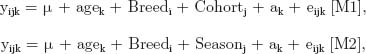
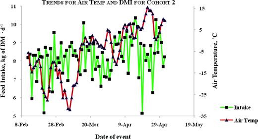
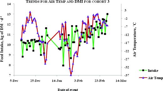
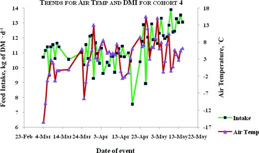
The correlation between air temperature and DMI was moderate and negative in season 1, but moderate and positive in season 2 (Table 6). The trends between air temperature and feed intake are illustrated in Figures 1, 2, 3, 4, and 5. Feed intake seemed to decline after sharp decreases in ambient temperature (Figures 3, 4, and 5). Feed intake (DMI) for animals tested in season 1 was correlated with the minimum and average measures of relative humidity (RH; P < 0.01), whereas season 2 animals did not show significant (P > 0.09) correlations between DMI and any measurement of RH. There were significant correlations between DMI and average, maximum and total solar radiation (P < 0.05) for season 1, whereas for season 2, significant correlations (P = 0.0109) were only observed between DMI and maximum solar radiation. Wind speed was significantly (P = 0.0495) correlated with DMI in season 2.
Estimates of correlation coefficients and associated significance levels for the correlation between climate variables and feed intake data for fall-winter and winter-spring seasons
| Item1 | Fall-winter | Winter-spring | ||
|---|---|---|---|---|
| Estimate | P-value | Estimate | P-value | |
| Maximum air temperature, °C | −0.26 | 0.001 | 0.27 | <0.0001 |
| Minimum air temperature, °C | −0.26 | 0.0008 | 0.33 | <0.0001 |
| Average air temperature, °C | −0.26 | 0.0011 | 0.31 | <0.0001 |
| Maximum RH, % | 0.00 | 0.9526 | 0.14 | 0.0949 |
| Minimum RH, % | 0.32 | <0.0001 | −0.08 | 0.3161 |
| Average RH, % | 0.23 | 0.0034 | −0.04 | 0.6598 |
| Maximum solar radiation, W/m2 | 0.19 | 0.0134 | 0.21 | 0.0109 |
| Average solar radiation, W/m2 | 0.30 | 0.0001 | 0.14 | 0.0957 |
| Total solar radiation, MJ | 0.30 | 0.0001 | 0.14 | 0.096 |
| Wind speed, m/s | −0.14 | 0.0712 | 0.16 | 0.0495 |
1RH = relative humidity.
Plots for trends of average air temperature and average daily DMI for animals tested in winter-spring of 2002–2003. Color version available in the online PDF.
Plots for trends of average air temperature and average daily DMI for animals tested in the fall-winter of 2003–2004. Color version available in the online PDF.
Plots for trends of average air temperature and average daily DMI for animals tested in the winter-spring of 2003–2004. Color version available in the online PDF.
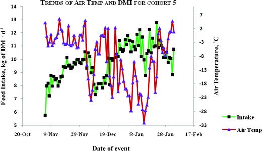
Plots for trends of average air temperature and average daily DMI for animals tested in the fall-winter of 2004–2005. Color version available in the online PDF.
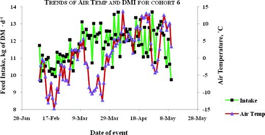
Plots for trends of average air temperature and average daily DMI for animals tested in the winter-spring of 2004–2005. Color version available in the online PDF.
Regression of mean climate parameters on DMI indicated that air temperature and RH had a significant effect on DMI in season 1 but not season 2 (P = <0.0001 and 0.1584, respectively). For season 1, average air temperature accounted for 5% of the variation in DMI, whereas average RH accounted for 3.3% (Table 7).
Parameter estimates (±SE) obtained by the regression of weather variables on feed intake in fall-winter and winter-spring test groups
| Item1 | Fall-winter | Winter-spring |
|---|---|---|
| Intercept | 8.89 ± 0.82 | 9.36 ± 0.82 |
| Cohort | −0.42 ± 0.08 | 0.08 ± 0.011 |
| Average air temperature | −0.02 ± 0.01 | 0.05 ± 0.02 |
| Average RH | 0.03 | 0.01 ± 0.01 |
| RSQ | 0.232 ± 0.01 | 0.03 |
| Model P-value | <0.0001 | 0.1584 |
| Item1 | Fall-winter | Winter-spring |
|---|---|---|
| Intercept | 8.89 ± 0.82 | 9.36 ± 0.82 |
| Cohort | −0.42 ± 0.08 | 0.08 ± 0.011 |
| Average air temperature | −0.02 ± 0.01 | 0.05 ± 0.02 |
| Average RH | 0.03 | 0.01 ± 0.01 |
| RSQ | 0.232 ± 0.01 | 0.03 |
| Model P-value | <0.0001 | 0.1584 |
1RH = relative humidity; RSQ = coefficient of determination.
2Average air temperature accounts for 5% of variation in DMI, whereas average RH accounts for 3.3%.
Genetic and phenotypic correlations between the different measures of RFI, performance, and behavior traits are shown in Table 8. Genetic correlations between RFIS, RFIC, and ADG were not significant given the large SE observed. However, there was significant correlation between RFIO and ADG. The correlations between RFIC or RFIS and DMI were moderate and within the range observed by other studies, whereas the correlation for RFIC was slightly greater. Feeding duration was not genetically correlated with RFI, whereas number of visits showed a high correlation. Ultrasound backfat did not have a significant correlation with RFI. Phenotypic correlations between RFI, UBF, and feeding duration were significant in contrast to genetic correlations. On average, ADG and MWT accounted for 60% of the variation in DMI.
Genetic and phenotypic correlations (±SE) among various measures of residual feed intake (RFI) and feed intake, performance, and behavior traits1
| Item | Genetic correlation | Phenotypic correlation | ||||
|---|---|---|---|---|---|---|
| RFIC | RFIO | RFIS | RFIC | RFIO | RFIS | |
| ADG | 0.21 ± 0.37 | 0.53 ± 0.46 | 0.31 ± 0.39 | −0.00 | 0.00 | 0.00 |
| DMI | 0.45 ± 0.29 | 0.68 ± 0.24 | 0.51 ± 0.28 | 0.56 | 0.63 | 0.58 |
| MWT | −0.33 ± 0.55 | −0.32 ± 0.59 | −0.27 ± 0.58 | −0.00 | −0.00 | 0.00 |
| UBF | −0.92 ± 1.05 | −0.79 ± 1.15 | −0.99 ± 1.20 | 0.19 | 0.23 | 0.17 |
| Duration | 0.03 ± 0.45 | 0.29 ± 0.41 | 0.04 ± 0.47 | 0.36 | 0.46 | 0.36 |
| Visits | 0.95 ± 0.31 | 0.64 ± 0.50 | 0.94 ± 0.34 | 0.25 | 0.16 | 0.21 |
| HDown | 0.46 ± 0.38 | 0.74 ± 0.35 | 0.51 ± 0.39 | 0.41 | 0.49 | 0.45 |
1Duration = length of time spent on a meal; HDown = head-down time; MWT = metabolic mid-BW; UBF = ultrasound backfat; visits = number of visits to the feed bunk; RFIO = RFI obtained by regressing ADG and MWT on DMI for each test group separately; RFIC = RFI obtained by regressing ADG and MWT on DMI on all pooled data, with test group as a fixed effect; RFIS = RFI obtained by regressing ADG and MWT on DMI, with test group as a fixed effect but within seasonal (fall, winter) groups.
Estimates of variance components, heritability, and EBV accuracy are shown in Table 9. Irrespective of the model used to evaluate RFI, RFIC had a better model fit, whereas RFIO had the least favorable fit based on the model LogL. Single trait direct heritability and EBV accuracy were greatest for RFIC and least for RFIO. In all instances, evaluation of the various RFI derivations with models M1 and M2 led to greater residual variance estimates for RFIO.
Variance component and genetic parameter estimates obtained from the genetic evaluation of the 3 measures of residual feed intake (RFI) using 2 different evaluation models1
| Item | Model M1 | Model M2 | ||||
|---|---|---|---|---|---|---|
| RFIC | RFIO | RFIS | RFIC | RFIO | RFIS | |
| Direct genetic variance | 0.15 | 0.12 | 0.13 | 0.13 | 0.14 | 0.14 |
| Residual variance | 0.47 | 0.56 | 0.50 | 0.48 | 0.61 | 0.53 |
| Heritability, h2a | 0.24 ± 0.17 | 0.18 ± 0.14 | 0.20 ± 0.16 | 0.22 ± 0.16 | 0.18 ± 0.14 | 0.21 ± 0.16 |
| EBV accuracy | 0.53 | 0.48 | 0.50 | 0.51 | 0.48 | 0.50 |
| Model Logl | −113.01 | −131.61 | −116.51 | −108.49 | −144.71 | −123.13 |
1RFIC = residual feed intake (RFI) obtained by regressing ADG and metabolic mid-BW (MWT) on DMI on all pooled data, with test group as a fixed effect; RFIO = RFI obtained by regressing ADG and MWT on DMI for each test group separately; RFIS = RFI obtained by regressing ADG and MWT on DMI, with test group as a fixed effect but within seasonal (fall, winter) groups.
DISCUSSION
In this study as expected, season 1 temperatures were less than season 2 temperatures because the fall-winter feed intake tests ended in January or February and thus span the coldest months (November, December, and January) in Alberta.
The average minimum air temperature in season 1 was close to the proposed critical body temperature (−20°C) for cattle (Young, 1981; NRC, 1996). Under thermoneutral conditions, the core body temperature (temperature of the inner body of the animal) is between 38 and 38.5°C (Sjaastad et al., 2003). Exposure to cold conditions below the critical body temperature has been associated with metabolic cold acclimatization, which results in increased resting heat production (Young, 1983). Lefcourt and Adams (1998) found that ambient temperature affected body temperature when a certain threshold was attained. In a separate study, Berman (2004) estimated significant increases in metabolic heat production as well as increased maintenance requirements due to exposure to cold at −10°C using published experimental data. Similar results were observed by several other studies reviewed by Young (1983) that attribute increased energy requirements in winter to enhanced resting heat production (RHP) brought about by the effects of cold climates on body core temperature. However, Kennedy et al. (2005) found no relationship between exposures to cold with metabolic acclimatization in crossbred beef heifers exposed for as much as 10 h·d−1 to −20°C conditions. Similarly, Birkelo et al. (1991) found no effect of season on maintenance requirements in Hereford steers. Nonetheless, various studies provide evidence suggesting that colder temperatures results in poor performance in terms of feed efficiency (Delfino and Mathison, 1991) and ADG (Birkelo et al., 1991).
In this study, the animals tested in season 2 were older and heavier at the start of the feed intake test, whereas ADG was not significantly different between the groups. To remove differences attributable to body size, the SWT was used to adjust growth and performance traits using Eq. [4]. Feeding behavior for season 1 animals (increased feeding duration, feeding events, and visits to the feed bunk) suggests increased feed intake, but reduced feed efficiency, compared with animals tested in season 2. More energy would be required for the increased feeding events especially because the animal would be more exposed to the elements, increasing the chances of heat loss. On a BW-to-BW basis, and considering the adjusted DMI estimates and intake per MWT, season 1 animals consumed more feed than season 2 animals, even though animals that are larger in size are expected to consume more feed. Given that this greater intake did not translate into faster growth rates (unadjusted ADG is the same for both groups), feed energy may have been allocated to mitigate the effects of harsh weather conditions, such as increasing heat production or accumulation of body fat to aid in insulation against heat loss. Season 1 animals had on average greater UBF thickness compared with season 2 animals.
The trend of increased feed intake with reducing air temperature is further supported by the negative correlations between DMI and air temperature. Correlations between DMI and solar radiation also suggest that feed intake increased with greater levels of solar radiation. The magnitude of this correlation was greater for season 1 compared with season 2, suggesting that the prospect of reduced heat loss may have encouraged animals to venture out to the feed bunks, as opposed to huddling together to conserve heat. Young (1981) suggests that the decreased critical temperature of a group of animals is much more reduced compared with that of a single animal. In their simulation study, Keren and Olson (2006) showed that in cold conditions, solar radiation is important in reducing the effects of extreme weather on metabolic requirements. On the other hand, wind velocity increases metabolic requirements due to the chill factor, such that ambient temperature feels much colder with greater wind speed. The negative correlations for season 1 suggest that days with greater wind speed accompanied by typically cold temperatures in that season may have led to a reduction in feed intake, by necessitating increasing huddling behavior or restricted movement by the animals so as to conserve body heat. Similarly, increased humidity may often result into wet hair coat for the animals, thus reducing insulation capabilities. For season 1, days with decreased humidity showed increased feed intake. On the whole, air temperature and RH had the greatest impact on feed intake in season 1. Regression of DMI on climate variables did not yield any detectable effects for season 2 despite the correlations observed between DMI and climate variables for this group.
Metabolic acclimatization to cold may possibly be a response to changes in core body temperature, and such changes affect energy partitioning. Individual animals are bound to show differences in metabolic adaptation to these changes. Given the differences in the correlation and regression parameter estimates for feed intake and climate variables in the 2 seasons, these results suggest possible differences in energy partitioning, adaptation, and hence efficiency of energy utilization in the 2 seasons. Consequently, RFI calculated in these 2 seasons may actually be indicative of 2 different traits, each capturing different components of energetic efficiency. However, because of the confounding affect brought about by animals in the 2 seasons being at different ages and BW, it is impossible to specify a cause-and-effect relationship between climate variables and feed intake.
Nonetheless, having observed differences in DMI, MWT, and UBF for the 2 groups, and possible individual animal differences in metabolic adaptation to cold conditions, it seems appropriate to group the cohorts into season 1 and season 2 groupings for genetic evaluation purposes. Furthermore, it also becomes necessary to assess how effective the various methods used to calculate RFI perform with respect to these groups. Normally, RFI is calculated as the differences between observed feed intake and EFI. Typically, EFI is predicted by regressing DMI on ADG, MWT and any other energy sinks (Crews, 2005) that show a correlation with RFI either within (Basarab et al., 2003) or across test groups (Arthur et al., 2001; Hoque et al., 2006). Some body composition traits such as ultrasound and carcass backfat (Arthur et al., 2001; Robinson and Oddy, 2004) and rib eye area (Hoque et al., 2005) have been shown to be associated with RFI. However, these correlations as reported in the literature are small in magnitude with large SE. A third way of deriving RFI is used here following the method of Arthur et al. (2001), but the regression is performed in each seasonal group separately. The reason for such an approach is to try and account for season-specific influences on DMI.
Within seasonal groups, RFIC and RFIS sum to 0, whereas RFIO does not. This is to be expected based on the methods applied. The genetic correlations between RFIC, RFIS and ADG, MWT were not significant. On the contrary, there was a significant correlation between RFIO and ADG. Even though RFI may be genetically correlated with ADG and MWT, the fact that RFIC and RFIS did not show this correlation and RFIO did points to reduced efficiency in minimizing the correlation between RFI and its component traits. Similarly, RFIO has a greater correlation with head-down time and weaker correlation with number of visits to the feeding bunk compared with RFIS and RFIC.
The stronger genetic correlations between RFI and number of visits or head-down time would imply reduced feed efficiency for animals tested in season 1, given that this group had a greater number of visits to the feeding bunk. Even though the magnitude of the differences between the correlations for the 3 measures of RFI is well within the range of the SE, there seems to be a trend that suggests that RFIO performs differently from the other 2 measures of RFI. Estimates of variance components using either model (M1 or M2) resulted in RFIC having the smallest residual variance and greatest estimates of heritability and EBV accuracy. Given the LogL, model M2 was best for evaluating RFIC and RFIO, whereas model M1 was suitable for evaluating RFIS. For RFIC, the results suggest that seasonal effects can be partly accounted for by including a season effect in the evaluation model (M2). For RFIO, however, trying to account for seasonal effects in the evaluation model results in the worst fit. These results suggest that the method of Basarab et al., (2003) leading to RFIC is the most suitable for evaluating RFI in animals tested in the 2 seasons. No matter what evaluation model was used, estimation of RFI by fitting a separate regression for each test group (RFIC) seems to be more consistent than when done within seasonal groups (RFIS). However, the method of Basarab et al. (2003) would fail when the intention is to assess increases in efficiency due to RFI selection. Typically, a single regression would need to be applied to all selection groups so that the progressive change in mean EBV with successive generations of selection is assessed. The method of Basarab et al. (2003) ensures that each group tested has a mean of null, whereas for the Arthur et al. (2001) method, each group will have a different mean allowing for changes in mean RFI value to be easily quantified as selection proceeds. Where selection has been undertaken and the population under study is tested for feed intake in different seasons, it is envisaged that the season-specific adjustments suggested in this study would become useful given no confounding factors.
The results in this study are suggestive of seasonal effects on feed intake and RFI estimation. However, because the 2 groups of animals started the tests at different ages, there is a confounding effect of age with season and it is hard to separate these 2 such that the differences in intake observed be wholly attributed to seasonal influences. The inclusion of age as a covariate in the evaluation model only allows a mathematical equalization to a common age (given that animals started the test at different ages) but does little to adjust for the real metabolic differences caused by the animals being at different physiological stages. Even though the differences in the estimated parameters cannot be wholly attributed to seasonal influences, it is apparent that feed intake measured in the 2 seasons relates differently to climate parameters, and the manner in which RFI is derived affects variance component estimation. However, as the drive to obtain more efficient cattle using RFI becomes intensified, more studies need to be conducted to understand how animals respond to environmental perturbations in situations of cold stress and how this may affect selection for NE efficiency.
Conclusions
This study sought to assess the influence of climate variables on feed intake and whether RFI calculated by regressing DMI on ADG and MWT in 3 different ways led to similar estimates of genetic parameters and variance components for young growing cattle tested for feed intake. There was a significant difference between fall-winter (season 1) and winter-spring (season 2) in mean climate variables to warrant separation of the tested cohorts into seasonal groupings. For season 1 animals, feeding behavior observed was indicative of increased DMI although unadjusted DMI was less than for season 2 animals. Correlation between climate variables and feed intake showed increased feeding with reducing temperature for season 1. Results obtained suggest that given no selection for RFI in previous generations, RFI is best estimated by regressing DMI on ADG and MWT for each test group separately, followed by genetic evaluation using a model that includes season as a fixed effect. However, confounding effects of age and BW of animals in the 2 seasons affected the results observed.
LITERATURE CITED
Footnotes
The study was made possible by grants awarded to Stephen Moore from the Canadian Cattleman's Association (Calgary), Alberta Agricultural Research Institute (Edmonton), Alberta Beef Producers (Calgary), Canada-Alberta Beef Industry Development Fund, and the Beef Cattle Research Council (Armidale, New South Wales, Australia).
