


Abstract
Viruses shape microbial community structure and activity through the control of population diversity and cell abundances. Identifying and monitoring the dynamics of specific virus-host pairs in nature is hampered by the limitations of culture-independent approaches such as metagenomics, which do not always provide strain-level resolution, and culture-based analyses, which eliminate the ecological background and in-situ interactions. Here, we have explored the interaction of a specific “autochthonous” host strain and its viruses within a natural community. Bacterium Salinibacter ruber strain M8 was spiked into its environment of isolation, a crystallizer pond from a coastal saltern, and the viral and cellular communities were monitored for one month using culture, metagenomics, and microscopy. Metagenome sequencing indicated that the M8 abundance decreased sharply after being added to the pond, likely due to forces other than viral predation. However, the presence of M8 selected for two species of a new viral genus, Phoenicisalinivirus, for which 120 strains were isolated. During this experiment, an assemblage of closely related viral genomic variants was replaced by a single population with the ability to infect M8, a scenario which was compatible with the selection of a genomic variant from the rare biosphere. Further analysis implicated a viral genomic region putatively coding for a tail fiber protein to be responsible for M8 specificity. Our results indicate that low abundance viral genotypes provide a viral seed bank that allows for a highly specialized virus-host response within a complex ecological background.
Introduction
Virus-host interactions shape microbial ecosystems [1], have profound effects on food webs and biogeochemical cycles, and are key determinants of microbial evolution thus linking evolutionary and ecological dynamics in microbial communities. Virus-host interactions are frequently very specific, both for the host and the virus, and depend on the community context [2]. At the level of individual virus-host pairs, interactions may proceed in a continuum between two extreme infection strategies: purely lytic and purely lysogenic [3, 4]. These interactions may translate, respectively, into two large scenarios in nature, known as Kill the Winner (KtW) and Piggy back the Winner (PbtW). In the KtW model, lytic infections are favored when host availability increases, keeping host diversity constant [5], whereas in the PbtW this increase will favor lysogeny and its ecological consequences. Both models have experimental support in different conditions and settings [6–8]. However, these are likely oversimplifications of the reality in which mixed approaches are adopted, either consecutively or simultaneous in different components of the community [9, 10], in combination with less characterized viral strategies such as pseudolysogeny or chronic infection [3]. Most importantly, how these interactions proceed have a strong dependence on the ecological communities involved and their biotic and abiotic interactions [1]. Compatible with these two scenarios, the Bank model suggests that most viral variants are present in the natural community at very low abundances and they only become (transiently) abundant when susceptible host increase their availability [11, 12].
The specificity of virus-host interactions may be undetectable using some community-focused approaches. Powerful as it is, short-read metagenomics cannot always assemble genomes from abundant viruses if levels of microdiversity are high. In fact, one of the most notorious cases is that of 37F-6, a marine virus that putatively infects Pelagibacter and is likely one of the most abundant viruses on the planet. This virus was unveiled only by the use of single-virus genomics since its genome had never been assembled from marine viral metagenomes due to its high level of microdiversity [13, 14]. Likewise, pairwise culture analyses, which have unparalleled power to explore interaction mechanisms, eliminate the community within which the virus-host interactions occur [1]. The temporal monitoring of medium complexity systems, such as mesocosms, can overcome some of the limitations of metagenomics and cultivation-based studies. This mixed approach allows the study of relatively controlled and natural systems and provides a sort of controlled “natural” experimental evolution setting [15].
Previously, some studies have been carried out to explore the evolutionary effects of the (normally simplified) community presence on focal cultured bacteria-phage species [2]. However, as pointed out by Ignacio-Espinoza et al. [16], “direct field observations of co-evolutionary outcomes are rare or limited to model systems”. Here, we have explored the interaction of a specific “autochthonous” host strain within a natural and diverse virus community, providing insight on the eco-evolutionary feedbacks occurring during virus-host dynamics. The system under study has been hypersaline brines (close to saturation) of a crystallizer pond from Es Trenc solar salterns in the Mallorca island (Balearic Islands, Western Mediterranean). The extreme environmental conditions in hypersaline ecosystems appear to drive their microbial communities into taxonomically similar assemblages with low diversities that are accompanied by highly dense viral communities. These prokaryotic assemblages generally consist of two major lineages: the archaeal Halobacteria class and the bacterial family Salinibacteraceae [17, 18]. Thus, hypersaline environments constitute tractable systems for studying virus-host interactions in natural settings. Within the Salinibacteraceae family, Salinibacter ruber was the first member of Bacteria demonstrated to grow actively and to high abundance in brines [19]. It is the dominant bacterium in many hypersaline systems worldwide although generally it is outnumbered by haloarchaea, in spite of being as halophilic as the most halophilic archaeon. This lower abundance could be due to viruses that control Sal. ruber populations in nature [20, 21].
Within the above mentioned framework, our goal was to explore the effects of the re-introduction of an autochthonous host on its natural community of cells and viruses. For this purpose, we added Sal. ruber strain M8 to a crystallizer pond from Es Trenc saltern, from where the strain had been isolated 15 years before, and monitored the community for one month. Our results showed how the increase of a suitable host was followed by a selection of initially very low abundance viral strains encoding specific genomic islands putatively involved in host recognition. In addition, drastically different outcomes were achieved by metagenomics and culture even for culturable host strains, stressing the complementarity of both approaches. The novelty of our work lies on the temporal monitoring of the evolution of phage-host interactions at the strain level against an ecological background, away from the lab environment.
Materials and methods
Experimental setup (pond description and sampling)
The mesocosm experiment was performed in August 2014 at the Mediterranean solar salterns of Es Trenc, located in Mallorca Island, Spain (39°20’N; 2°59′E), where two crystallizer ponds like the ones used for salt exploitation were prepared (Figs. 1A and1D). The first crystallizer, called Control pond, was used to study the natural dynamics of microbial communities and was left unamended along the experiment. The second one, named Sal. ruber strain M8 pond, was inoculated with 1.83X10¹³ cells of Sal. ruber M8 pure culture, ~9.3% of total cell counts (see below for the inoculum preparation details). The volume of brine in each ponds was, approximately, 15.2 m3 for the control pond, and 7.2 m3 for the amended pond. Both ponds were filled up to 40 cm approx. The ponds were built in 2012 and have been operating as the rest of crystallizers in the salterns since then, using the brines from the system of concentrator ponds that had been working for decades. Sal. ruber M8 was isolated from the Es Trenc saltern 15 years before the experiment [19] but was below the detection limit at the time of inoculation as checked using strain specific primers 156 [22].
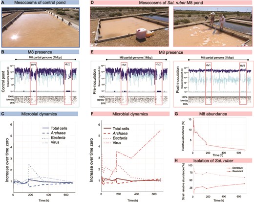
The experiment. (A) Control pond. (B) Recruitment of the genomic region of Sal. ruber containing the strain specific regions HV1 and HV2 against reads from the metagenome retrieved from the control pond at the beginning of the experiment. (C) Microbial dynamics in the control pond throughout the experiment tracked using total cell counts by DAPI staining, archaea and bacteria counts by CARD-FISH with domain specific probes, and virus counts as VLP detection by Sybr gold staining followed by epifluorescence microscopy. For each parameter, the variation respect to the initial time is given. (D) Pond amended with the Sal. ruber M8 culture. (E) Recruitment of the genomic region of Sal. ruber containing the strain specific regions HV1 and HV2 against reads from the metagenomes retrieved from the M8 pond before (t = 0) and after (t = 4 h) adding the strain M8 to the pond. (F) Microbial dynamics in the M8 pond measured as shown for the control pond in B. (G) Dynamics of M8 in the pond throughout the experiment measured as percentage of metagenomic reads recruited by the strain specific regions. (H) Sal. ruber strains isolated from the M8 pond which were sensitive or resistant to Phoenicisalinivirus.
The experiment was monitored for one month and the ponds were periodically sampled (including the sampling time right before and after Sal. ruber M8 addition, see Supplementary Fig. S1). During the first week, samples were taken every 24 h and then weekly. A total of 13 brine samples were taken from each pond, five of which were studied in more detail. At 168 h, because they were drying out due to evaporation, ponds were refilled (using the same brine for both ponds), a standard procedure in solar saltern management.
Biological replicates were not obtained due to the large volume and frequent sampling required in the mesocosms, making replication prohibitively expensive. Moreover, replication is generally unnecessary in time-series experiments like ours, where microbial community variability tends to be relatively small [23], as shown in previous time-series studies of hypersaline samples [24].
Sal. ruber M8 inoculum preparation and isolation along the experiment
A pure culture of Sal. ruber M8 was grown in 25% sea water (SW), 0.2% yeast extract (YE), pH 7.2 at 37°C as previously published [19]. The inoculum was checked using strain-specific primers [22] and a pool of primers specific to Salinibacter spp. or Archaea to guarantee its purity. Finally, 64 liters of pure M8 inoculum were concentrated to 35 liters by Vivaflow 100 K ultrafiltration in order to facilitate its transport from Alicante to Mallorca. Inoculum cell concentration was determined by DAPI staining [25].
Sal. ruber M8 was isolated along the experiment by plating brine samples in 25% SW + 0.05% YE agar plates at 37°C and checking the individual colonies with M8 specific primers.
Isolation of M8 viruses from mesocosm experiments
Exponentially grown M8 cultures were directly mixed with 0.7% agar in 25% SW and poured into 25% SW + 0.2% YE agar plates. Viral assemblages were prepared after centrifuging brines to pellet cells at 13000 rpm and filtering the supernatants through 0.22 μm filters. Then, 5 μl of these viral preparations, were separately spotted, directly and after decimal serial dilution (down to 10−6 of the initial concentration), on top of the Sal. ruber M8-soft agar layer. Virus isolation was carried out with samples from M8 and control ponds, as well as from another crystallizer pond of the system (E2), amended with Sal. altiplanensis strain PH3 [26], which was not otherwise used in this work. The resulting spot-plaques were then collected from the soft agar, suspended in 25% SW, mixed thoroughly, and used for further virus purification using the double layer technique (See Supplementary Methods for more details of the process).
Microbial and viral counts and nucleic acid extraction
Cells and viruses were counted by DAPI and Sybr Gold staining [20, 21, 27], and the proportion of Archaea and Bacteria determined by FISH (Antón et al., 1999). Details are provided in the supplementary methods.
For cell DNA extraction, 25 ml of brine samples were centrifuged at 13000 rpm and DNA was extracted from the pellet as detailed previously (Urdiain et al., 2008). For RNA extraction, pellets were stored in RNAlater solution (Invitrogen, Thermo Fisher Scientific, Lithuania) at −80°C until processed. The PowerMax Soil DNA kit for extracting RNA was used for total RNA extractions (MoBio) and TURBO DNAse (Ambion) to remove DNA. More details are provided in the supplementary methods.
Sequencing and preliminary viral metagenome analyses
Sequencing of viral DNAs was performed using a MiSeq Nextera XT run (2x300bp, paired-end reads; Illumina) and isolated viral genomes were sequenced separately using Nextera libraries and a MiSeq SEQ 500 Hi-output sequencing run (Illumina). Reads were quality assessed and trimmed using PRINSEQ v0.20.4 software [28] (min_length 50, trim_qual_right 20, trim_qual_type mean, trima_qual_window 20) and paired-end reads were joined using fq2fa from IDBA v1.1.1 assembler [29]. Only reads larger than 50 bp and with a quality over 20 were considered for further analyses. The Nonpareil v2.4 tool [30] was used to estimate the coverage of the community in each metagenome dataset with default parameters. De novo assemblies of trimmed reads were generated using the IDBA v1.1.1 assembler [29] with the “-pre_correction” option.
Sequencing and initial cell metagenome and metranscriptome analyses
Sequencing of cell DNA was performed using an MiSeq (2 × 250 bp, paired end reads; Illumina) and HiSeq (2 × 100 bp, paired end reads; Illumina) instruments. SolexaQA tool v3.1.4 [31] was used to trim the paired-end reads with a quality score below 20 and reads with <50 bp lengths were discarded. The trimmed reads were assembled with the IDBA v1.1.1 assembler [29] with the “—pre-correction” option. Genes from the assembled contigs with length > 500 bp were predicted using MetaGeneMark.hmm v3.25 [32]. Protein-coding genes were annotated against the UniProt database using BLASTp 2.2.30+ [33], considering the best match to have >40% amino-acid identity, >70% sequence length compared to the reference sequence and a bit-score higher than 60. For phylogenetic purposes, the reads associated with 16S rRNA genes were extracted using the Parallel-META v2.4 tool [34] and clustered at 98.7% similarity using QIIME v1.9.1 script pick_closed_reference_otus.py to identify Operational Taxonomic Units (OTUs). The representative sequences from each OTU were aligned using the SINA tool v1.3.1 [35] and were added to the reference database SILVA REF 128 [36] using the parsimony method implemented in the ARB software v6.0.6 [37]. The OTUs were then clustered into OPUs (Operational Phylogenetic Units) as recommended [38].
For metatranscriptome analyses, RNA was retrotranscribed to cDNA and sequenced. Metatranscriptomic sequences were cleaned by Prinseq v0.20.4 (−fastq -fastq2 -verbose -derep 12 345 -lc_method entropy -lc_threshold 70 -out_format 3 -min_len 20 -trim_qual_right 15 -trim_qual_left 15 -trim_qual_window 2 -trim_qual_step 1 -min_qual_mean 20 -ns_max_p 1 -noniupac -out) (Cantu et al., 2019). Following, the 16S rRNA gene sequences were identified and removed by rnascan v 2.0.0 (−moltype ssu,lsu,tsu). The trimmed metatranscriptomic reads were mapped against Sal. ruber M8 and M8 isolate virus genomes by Bowtie v9.3.0 (Langmead and Salzberg, 2012) and Tophat library-type fr-firststrand —no-novel-juncs (Trapnell et al., 2009). The outputs were filtered using the Samtools v1.10 collection (depth –aa –d 10 000 000) (Weeks and Luecke, 2017).
Cell and virus metagenome annotation and comparison
Functional annotation of predicted genes from cellular and viral assembled metagenomes was done using the JGI IMG/MER platform [39], DIAMOND BLASTp v0.9.28. [40] and interpro 5.41–78.0 [41]. In addition, the NR NCBI database (December 2019 update) and the UniProt database [42] were used for viral and cell metagenomes, respectively. Raw cell and viral metagenomes “all versus all” comparisons were performed by BLASTn 2.9.0 stand-alone considering only best-hit matches over 70% of read coverage. Additionally, metagenome raw read comparisons were performed by MASH v1.1 (parameters for sketch: -s 10000 -r -m 2) [43] and Metafast v1.3 [44].
Viral genome comparisons and clustering
After viral DNA extraction and sequencing (see supplementary methods.), whole viral genome comparisons (in nucleotides) were performed by VIRIDIC [45] and ORF comparisons between reference viral genomes were analyzed using an amino acid reciprocal best match strategy (rbm.rb, enveomics collection) [46]. Heat maps and boxplots were drawn by Plotly by R (Plotly Collaborative Data Science 2015 Data Storytelling Studio @ MIT). Whole viral genome alignments were drawn using the Easyfig platform [47]. Viral proteomic tree including published viral genomes was built using VIPtree [48].
The first clustering step was performed using cd-hit-est v4.8.1 (−c 1, n 8, aL 0.8) [49], considering only genomes larger than 43 kb (this threshold was chosen based on the viral genome sizes determined by PFGE). Briefly, ANI was performed by VIRIDIC [45] and Jspecies [50]. The non-redundant 120 viral genomes were clustered again according to their reciprocal AAI (average amino acid identity). The AAI of each genome was calculated by reciprocal best match of all versus all ORFs in amino acids (rbm.rb, default parameters by enveomics collection [46] and additionally the ANI of each complete genome was calculated. Finally, viral genomes were clustered using a dissimilarity matrix based on AAI values between genome pairs (Bray Curtis) [51] and the largest and most complete genome of each cluster was selected as “group reference genome”.
Cell and viral genome abundances
Cell and viral abundances, as well as the absence, presence, and permanence of M8 during the experiment were calculated by fragment recruitment of each genome in each metagenome (cell or virus) by BLASTN v2.9.0 (cut-off >70% coverage, −evalue 0.1 and filtered with the BlastTab.best_hit_sorted.pl script from the enveomics collection). The BlastTab.seqdepth.pl script, also from the enveomics package [46], was used to calculate the sequencing depth of the genomes. Isolated viral abundances (viral genotype abundance) were calculated as a percentage of total recruited nucleotides in each metagenome (% of total nucleotides were performed as recruited nucleotides/total metagenome nucleotide size × 100) and normalized by viral genome size (Kbp), only reads mapped over 70% of coverage and 100% of identity were considered. Recruitment plots were drawn with R (enveomics.R library) [46]. Finally, the abundance fold change between different times was calculated as (abundance in time X/ abundance time Y) when X is a selected time point n and Y is the previous time n-1.
Proteomic analyses of the new viral isolates
In order to refine the annotation of the viral genomes, structural proteins (i.e. present in the virion) were analyzed by orbital mass spectrometry on digested virion extracts. The detected proteomes were mapped into a custom proteomic database including the non-redundant ORFs from isolated viral genomes. More details are provided in the supplementary methods.
Viral genome diversity analyses (SNPs and pN/pN + pS)
To calculate the percentage of polymorphisms in the isolated viral genomes, raw reads from each viral metagenome were mapped against isolated viral genomes separately (only reference genomes) using the sensitive local mode of Bowtie2 V 2.4.4 (Langmead and Salzberg, 2012). Then, in order to obtain counts of synonymous and nonsynonymous mutations in each ORF, the output files were analyzed by DiversiTools (−-min_aa_cov 5 --min_mut_codon_count 4 --min_mut_codon_freq 1) (http://josephhughes.github.io/DiversiTools/). Only ORFs shared between the control and M8 ponds were considered. Details on downstream analyses are provided in the supplementary methods.
qPCR and amplicon sequencing analyses of selected viral genes
The abundance of the newly isolated Phoenicisalinivirus was measured in the control and M8 pond by qPCR with two primers pairs targeting, respectively, the highly conserved tail fiber protein gene (primers C) and a highly diverse structural protein gene (primers VR, from “variable region”). All qPCR amplifications, including those of the standard curve, were carried out in triplicate. See supplemental methods for further details.
The diversity of these viruses was monitored by a metabarcoding analysis using these two primers pairs with the appropriate adapter for Illumina sequencing. More details are provided in the supplementary methods. Sequences were quality filtered by employing Trimmomatic v0.36 [52] (ILLUMINACLIP:NexteraPE-PE.fa:2:30:10 LEADING:3 TRAILING:3 SLIDINGWINDOW:4:15 MINLEN:36) and joined with FLASH v1.2.11 using default parameters [53]. To remove spurious sequences, only those sequences that aligned against viral genomes (BLASTn v2.9.0+, minimum e-value 1e-10) were analyzed. FastA.sample.rb from the Enveomics collection [46] was employed to normalize samples to 11 421 sequences for primers C, and 61 195 sequences for RV to allow comparisons between them. Then, sequences were clustered at 100% identity and coverage with cd-hit-est v4.8.1 (−as 1 -c 1) [49], the Shannon index was calculated by the phyloseq R package v1.40.0 [54] and finally, the plot was drawn in R with ggplot2 v3.4.2 [55].
Host range
The host ranges of the 10 reference viruses against a panel of different Sal. ruber strains were determined by the spot test technique [21]. The susceptible and resistant hosts were detected with a spot test applying cell-free phage lysates over agar-overlays of individual host lawns. Susceptibility to the viruses was verified by plaque assay. The plates were incubated as described above.
Results and discussion
Experiment set-up and monitoring community dynamics
Two ponds (hereafter “control” and “M8 pond”, Figs. 1A and1D) were chosen for the experiment based on the undetectable levels of strain Sal. ruber M8, as determined by PCR with M8-specific primers, which can detect in the order of 103 cells/ml (as estimated by using serial dilutions of a Sal. ruber M8 culture), and further confirmed by metagenomic analyses (Figs. 1B and1E 1, see below). M8 cells from a pure culture were added to the M8 pond to a final concentration of 9.3% of total cells whereas nothing was added to the control pond. Strain M8 had been isolated in 1999 from these salterns [19], and therefore can be considered part of their autochthonous microbiota and had the opportunity to interact and coevolve with the salterns’ cell and virus assemblages in the past.
The ponds were monitored during a 672-h period, with a higher sampling frequency at the beginning of the experiment (Supplementary Fig. S1). At 168 h, due to evaporation, the ponds were drying out and had to be refilled (using the same brine for both ponds, which caused a decrease in salinity of 4–7% units approx., see Table S1), a standard procedure in solar saltern management. It is important to notice that the refilling brine came from the concentrator pond used for feeding all the crystallizers. In both M8 and control ponds, cell counts returned to their time zero numbers by the end of the experiment while virus counts increased only in the M8 pond (Figs. 1C and1F, and Table S1).
The fate of M8 in the M8 pond was followed by metagenomic recruitment of M8-specific genomic regions, known as hypervariable regions 1 and 2 [22], labeled as HV 1 and 2 (Figs. 1B and1E, andS2). This analysis also confirmed the absence (or abundance below the sequencing detection limit, that at this sequencing depth is 2.105 genomes/ml calculated as in [56]) of the strain in the system prior to the experiment (Fig. 1E, Fig. S2A), in good agreement with the previous PCR with strain specific primers. Following M8’s addition to the pond, its abundance steadily decreased, reaching, by the end of the experiment, an almost residual abundance (less than 0.4% of the metagenomics reads). This decrease of M8 did not imply that the added M8 was inactive, as shown by genome recruitment against metatranscriptomic reads of the cellular assemblage (Fig. S2B). The decrease of M8 density is predicted by classical ecological theory [57] and can be explained as an outcome of either competition and/or viral predation.
The analysis of cellular and viral metagenomes (Tables 1 and 2 for their general traits) indicated how the addition of M8 impacted both cellular and viral assemblages (Fig. S3); distances between whole metagenome read comparisons (MASH distances in Figs. S3A, B, and D) showed that M8 addition had a larger effect on the cellular than the viral community (Fig. S4). However, although the initial communities were different in each pond, pointing to a certain degree of stochasticity in the system, the taxonomic profiles of both crystallizers at the end of the experiment were very similar to that of their respective initial communities (Fig. S3C). A similar stability was observed in different experiments carried out in 2012 and 2014 in crystallizer ponds from the saltern system analyzed here [24].
Characteristics of the viral metagenomes used in this study.
| Pond | Metavirome ID | Time (hours) | Reads | Total nucleotides | %GC | Nonpareil values (diversity/coverage) | 16S rRNA gene proportion (%) | Assembly size (Mbp) | Q20/Q30 | Min/max (bp) | Contigs | Assembled (%) |
|---|---|---|---|---|---|---|---|---|---|---|---|---|
| Control pond | Control T0h | 0 | 1 314 648 | 271 550 874 | 53.5 | 16.24/87.87% | 0.018 | 26.5 | 98.4/93.4 | 100/22350 | 62 040 | 21.5 |
| Control T72h | 72 | 1 307 290 | 262 782 463 | 55.5 | 16.9/76.7% | 0.05 | 26.7 | 98.5/93.6 | 100/40208 | 595 588 | 21.4 | |
| Control T168h | 168 | 1 340 470 | 262 122 041 | 55 | 16.78/83.4% | 0.04 | 25.7 | 98.6/94 | 100/28633 | 54 615 | 21.3 | |
| Control 169 h | 169 | 1 498 842 | 304 765 505 | 54.4 | 16.52/86.1% | 0.05 | 29.7 | 98.5/93.6 | 100/34056 | 60 010 | 24.5 | |
| Control T672h | 672 | 731 830 | 145 710 123 | 57 | 16.5/82.1% | 0.05 | 15.49 | 98.5/93.7 | 100/23854 | 31 382 | 20.9 | |
| Sal. ruber M8 pond | S. ruber M8 T0h | 0 | 990 508 | 220 721 760 | 53.7 | 16.9/90.4% | 0.002 | 21.0 | 98.3/96 | 100/18155 | 57 625 | 24.1 |
| S. ruber M8 T72h | 72 | 2 611 956 | 575 669 555 | 54.8 | 15.7/93.6% | 0.005 | 4.8 | 98/91 | 100/31905 | 149 598 | 24.7 | |
| S. ruber M8 T168h | 168 | 1 961 392 | 439 592 060 | 50.3 | 17.1/93.3% | 0.001 | 36.42 | 98/91.8 | 100/38302 | 111 380 | 24.7 | |
| S. ruber M8 T169h | 169 | 1 859 328 | 407 296 917 | 54.4 | 16.6/88.2% | 0.001 | 40.5 | 98.4/93 | 100/34260 | 100 265 | 25.5 | |
| S. ruber M8 672h | 672 | 1 977 784 | 438 021 570 | 52.2 | 16.5/92.1% | 0.001 | 45.2 | 98.5/93.4 | 100/263015 | 108 222 | 28.9 |
Characteristics of cellular metagenomes.
| Pond | Metagenome ID | Time (hours) | Reads | Total nucleotides | %GC | Nonpareil values (diversity/coverage) | Assembly size (Mbp) | Contigs |
|---|---|---|---|---|---|---|---|---|
| Control pond | Control T0h | 0 | 337 702 | 66 195 891 | 55.738 | 17.77/42.1% | 6.3 | 4555 |
| Control T72h | 72 | 528 468 | 103 434 888 | 56.441 | 18.08/44.61% | 10 | 6885 | |
| Control 169 h | 169 | 997 812 | 196 400 422 | 55.217 | 17.77/58.23% | 17 | 11 691 | |
| Control 360 h | 360 | 788 212 | 151 486 662 | 56.668 | 18.18/48.89% | 13 | 10 898 | |
| Control T672h | 672 | 1 142 478 | 229 346 011 | 55.963 | 18.11/55.66% | 19 | 14 875 | |
| Sal. ruber M8 pond | S. ruber M8 T0h | 0 | 497 798 | 95 137 015 | 57.082 | 18.1/43.86%3 | 12 | 9248 |
| S. ruber M8 T72h | 72 | 453 732 | 95 392 451 | 58.540 | 17.61/52.62% | 12 | 7539 | |
| S. ruber M8 T168h | 168 | 384 504 | 83 688 457 | 57.584 | 17.91/44.22% | 11 | 7909 | |
| S. ruber M8 T169h | 169 | 40 273 294 | 3 797 761 300 | 61.898 | 18.2/85.95% | 94 | 64 502 | |
| S. ruber M8 t 360 h | 360 | 28 844 742 | 2 708 447 940 | 58.114 | 17.97/87.4% | 71 | 51 579 | |
| S. ruber M8 672h | 672 | 110 992 232 | 2 209 258 135 | 55.4 | 18.08/83.5% | 94 | 85 892 |
Retrieval of viruses infecting Sal. ruber M8
Two strategies were used for M8 virus retrieval: the identification of metagenomic viral contigs corresponding to putative Sal. ruber viruses and the isolation of Sal. ruber M8 viruses by plaque assays.
Viral contigs were retrieved from the viral metagenomes of both the control and the M8 ponds (Dataset S1, Fig. S5), and their relative abundances along the experiment were calculated. Only contigs larger than 10 Kb whose relative abundances increased along the experiment more in the M8 than in the control pond were selected for further study. The rationale was to select genomes corresponding to virulent viruses that would increase their abundance as a result of M8 infection and lysis. However, except for their relatively high GC content (also common in most haloarchaeal viruses), genomic analyses did not unveil any trait (e.g. CRISPR protospacers and tRNAs) that could unambiguously identify them as infecting Sal. ruber. Therefore, this strategy was disregarded, and a culture-dependent approach was undertaken instead.
Viruses infecting M8 were isolated by the plaque assay technique using filtered brine as a direct source of viruses, as previously described ([21]; methods). Viruses infecting M8 could be isolated from the M8 pond, at time points 336 (40 plaques) and 672 (132 plaques). Not a single M8 virus was isolated from control pond brines (Dataset S2 and Table S2). Furthermore, an additional set of 27 viruses infecting M8 could be isolated from a contiguous pond (named E2, supplementary results), after 672 h post inoculation. Thus, a total of 199 plaques were obtained from three different samples (Dataset S2).
Genomic characterization of the Phoenicisalinivirus: A new genus of viruses infecting Sal. ruber M8
A total of 190 virus genomes were sequenced and, of these, 120 were non-redundant complete viral genomes (Table S2). Overall, the 120 genomes formed a genetically homogenous group, which, according to VIRIDIC (Fig. S6A), constituted two species from the same viral genus. One species was represented by only one genome, B2_17, whereas the second species comprised the other 119 viruses, which formed nine different groups (i.e. intra-species clusters) based on amino acid identity (Fig. S6B). One representative of each of the nine groups (i.e. nine strains from the same species), together with virus B2_17, were selected for detailed phenotypic and genotypic characterization. Virions from each representative had a head and tail morphology resembling myoviruses (Fig. S7) with head diameters around 66 nm and tail lengths of 120 nm, slightly larger than the previously isolated Sal. ruber phages [21]. Viral particles were not sensitive to chloroform (supplementary methods for the protocol description), likely indicating that they had no lipid envelopes.
The genomes of the newly isolated viruses infecting Sal. ruber M8 had sizes and GC contents of 44–46 Kb (confirmed by PFGE) and 63%, respectively, and presented terminal redundancy. They had no homology at the nucleotide level with any previously isolated virus present in databases, including those infecting Salinibacter (Fig. S8 for a proteomic tree). According to ICTV guidelines (two phages are assigned to the same species/genus if their genomes are more than 95%/70% identical at the nucleotide level over their full genome length, tested reciprocally [58–60]), these viruses belonged to two new species (Fig. S8) within the Caudoviricetes class, and formed a new genus for which we propose the name Phoenicisalinivirus. The genus name comes from the Phoenix bird in the Greek mythology which regenerated from its ashes cyclically. The two new species are named P. gymnesicum and P. balearicum, in reference to the Greek and Latin names, respectively, of the place of isolation (Mallorca, Balearic Islands, Spain). Around one half of the ORFs in the new Phoenicisalinivirus genomes could be annotated, either in silico or by the identification of structural proteins by mass spectrometry (Fig. 2, Supplementary Dataset S3). A more detailed description of the genomic characteristics of Phoenicisalinivirus is provided in Supplementary Results.
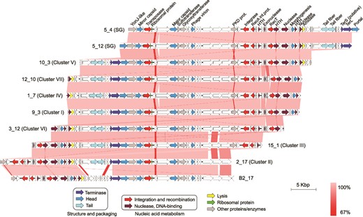
The Phoenicisaliniviruses. Genomic organization of the phoenicisaliniviruses. Every ORF is colored according to its predicted function (see legend). Lines connecting genomic regions are colored according to their nucleotide identities.
The genomes of both viral species displayed regions of high gene identity and synteny, as well as species-specific regions corresponding with the metagenomic islands discussed below, as an additional example of the typical mosaicism observed in viral genomes (Fig. 2). The comparison of the representative viral genomes within the species P. gymnesicum, from which we had a high number of genomes to compare (i.e. 119 genomes in the nine clusters mentioned above, whereas only one genome corresponded to P. balearicum), indicated that, despite their relatedness, there were genomic regions where differences accumulated whereas other regions were extremely conserved (Fig. 2 and Supplementary Fig. S9). Genes coding for proteins identified as structural were overall more conserved than genes encoding other or unknown functions (Fig. S9, the equivalence in genes labeling among the different isolates can be found in Dataset S3). Conversely, several hypothetical proteins displayed high levels of variation between the different virus groups. A similar trend has been observed when studying uncultured viruses infecting a natural bloom of green sulfur bacteria [6]. These regions of variability do not seem to affect host specificity of P. gymnesicum although they could potentially affect future adaptation to new hosts, as shown by experimental genomic evolution of phage-host pairs [61].
None of these genomes had any similarity to the viral contigs (larger than 3 Kb) assembled from their corresponding viral metagenomes, likely due to the high microdiversity of the population and low relative abundance (e.g., see recruitment plots in Fig. S10), together with the presence of both species-specific and shared genomic regions. As mentioned above, this is a well know limitation of viral metagenomics [21, 62, 63].
To ascertain to which extent these isolated viral genomes represented their “natural” populations and could thus be used for a meaningful monitoring along the experiment, we first retrieved these populations by selecting all metagenomic reads mapping above 95% identity with the isolate genomes in the metavirome of the Sal. ruber amended pond at time 692 h. This value has been previously considered as the threshold for a viral species/population [64, 65]. Then, the fraction of the population retrieved by culture was ascertained by quantifying the reads matching with 100% identity against the isolate genomes. The rationale was thus to retrieve first the reads accounting for each viral species-like population and then to ascertain the fraction of these reads corresponding to the isolated genomes. The viral isolates of the species P. gymnesicum and P. balearicum represented around one half of the diversity (46.9 and 46.4% of the reads representing either species, respectively) in the viral metagenomic reads from their respective natural populations. In other words, culture allowed the retrieval of around one half of the natural species-like population diversity for both viral species. Thus, the isolated viral genomes could be considered as good representatives of their natural populations and were used to monitor viral-host dynamics.
Dynamics of phoenicisaliniviruses involves the selection of a viral genomic variant
Changes in phoenicisaliniviruses assemblages along the experiment were monitored by recruiting isolated genomes against cellular and viral metagenomic reads from the control and M8 ponds. The recruitment plots showed some genomic regions of low recruitment at the beginning of the experiment that, in pond M8, subsequently experienced an increase in coverage. Thus, complete P. balearicum and P. gymnesicum genomes could not be detected by metagenomics in the pond before inoculation, although closely related viruses (i.e., sharing part of their genomes with phoenicisaliniviruses) were present. The following analyses focus on the dynamics of the species P. gymnesicum, given also that the dynamics of P. balearicum was similar (see the corresponding recruitment plots in Fig. S10).
In more detail, a region specific to the P. gymnesicum genome and highly conserved in all isolated viruses (marked with an asterisk in Fig. 3) showed extremely low coverage at the beginning of the experiment in both ponds, and was replaced at the end by a homogenous sequence coverage only in the amended pond (Fig. 3). This was observed for the recruitments with both the viral and the cellular metagenomes from the amended pond, indicating that the selected genomic variants were present both within extracellular virions and actively replicating within the host cells. This pattern was not observed in the control pond (see the corresponding recruitment plots in Figs. 3 and S10).
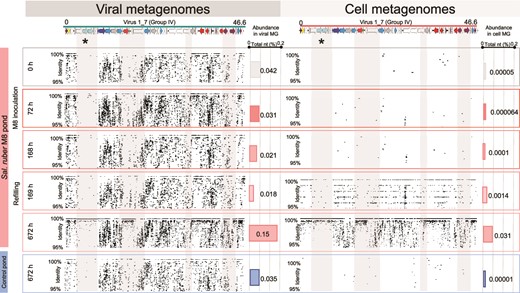
Dynamics of Phoenicisalinivirus gymnesicum throughout the experiment. Recruitment of reads to a Phoenicisalinivirus gymnesicum genome. Reads are from the viral (left) or cellular (right) metagenomes sampled at different times during the experiment in the M8 pond. The asterisk marks the region coding for the putative tail protein.
Annotation indicated that, among the genes within this conserved region, there were two ORFs (colored light blue in Fig. 2) identified as “putative tail fiber protein”. Furthermore, the corresponding proteins could be detected by mass spectrometry in the isolated phages and were therefore structural. Tail fiber proteins are very frequently involved in host recognition and may be responsible for virus specificity [66]. Thus, this genomic region could be involved in host interaction and be responsible for specificity of P. gymnesicum for their host. Our results suggest that a genome encoding a variant of the tail fiber protein was selected throughout the experiment, as its sequence became less diverse (as indicated by the recruitment plots) and more abundant over time, as previously shown in other systems [1]. Another clue that suggests this region was involved in host recognition was provided by the genomic comparison of the two isolated virus species which indicated that both viral species differ in this region and had (slightly) different host ranges (Fig. 2), as discussed below. Thus, metagenomic recruitments of the isolated viruses suggested that an assemblage of closely related genomic variants of P. gymnesicum with the ability to infect M8 was selected along the experiment.
Tail fiber gene amplicon sequencing and qPCR analyses provide higher resolution into Phoenicisalinivirus population dynamics
The increase of the M8-infecting viral population was confirmed by qPCR with a primer set targeting one of the genes coding for the putative tail fiber (CCDS09 in the annotation dataset S3). Both metagenomic and qPCR analyses yielded similar patterns (Fig. 4). These results also indicate that metagenomics did not have enough sensitivity to detect this virus population initially, a phenomenon that must be kept in mind when analyzing shotgun metagenomic datasets. The higher sensitivity of qPCR compared to metagenomics has been previously documented for the detection in natural samples of specific viruses or antibiotic resistance genes [67–70]). In fact, the limit of detection of metagenomics has been estimated to be, at least, two orders of magnitude higher than that of PCR based methods, depending on the relative abundance of the targeted organism and the sequencing effort applied [71]. Thus, unless sequencing is performed at a sufficient depth, metagenomics may not be useful to distinguish between genetic evolution due to immigration, or fluctuation or selection of previously existing (but low relative abundance) genetic variants. Therefore, caution must be exerted when over-interpreting metagenomic data.
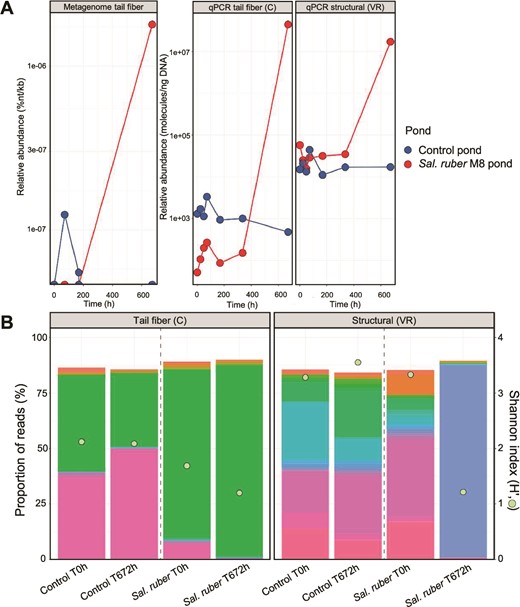
Phoenicisalinivirus gymnesicum abundance and diversity along the experiment. (A) Abundance of P. gymnesicum in the M8 (red lines) and control (blue lines) ponds calculated as normalized percentage of the viral metagenome reads (left panel), copies per nanogram of DNA measured by qPCR with primers specific for the gene coding for the tail fiber protein (central panel), and with primers targeting a more variable region encoding for a structural protein (right panel). (B) Diversity of the tail fiber (left) and the structural protein (right) genes at times 0 h and 672 h as estimated by amplicon sequencing using extracellular viral DNA as the target and primers used in A. The bar plot represents the relative abundance of different phylotypes (in different colors) detected by amplicon sequencing measured as percentage of reads. Phylotypes were called by sequence clustering at 100% identity and coverage. A total of 57 and 77 phylotypes were identified for the tail fiber (C) and the structural protein (VR) genes, respectively. Green dots represent the Shannon index (H′).
To ascertain whether there was selection of a previously available genotype or, less likely, evolution of the previously present virus, which would allow it to infect a new host, the diversity of viral genomes was tracked throughout the experiment using a amplicon sequencing approach. For this purpose, DNA from the ponds was amplified with the above mentioned primer set conveniently modified for amplicon sequencing analyses of their corresponding amplicons. A clear decrease of the diversity of the tail-fiber coding gene was observed in the amended but not in the control pond (Fig. 4B, left panel). This decrease in diversity was due to the selection of a sequence previously present in the system, which relative abundance increased only in the M8 pond and corresponded to that of the isolated viruses. Thus, the presence of strain M8 selected for a subset of viruses initially present at low concentration which carried the gene coding for the tail fiber protein that likely mediates host specificity.
For comparison, qPCR and amplicon sequencing analyses were also carried out with primers VR targeting a gene less conserved in the P. gymnesicum genomes (CCDS24 in Dataset S3). Most likely, as indicated by the recruitment plot and qPCR (compare qPCRs in Fig. 4A), this region was shared with other viruses initially present in the system. Amplicon sequencing analyses indicated that, at the end of the experiment, there also was a relative increase in the amended pond of a previously present sequence variant (right panel in Fig. 4B). This observation is compatible with a selection (and increase) of genomes carrying the tail fiber protein gene which would in turn select for the rest of the genes in the genome. This would explain why, at the end of the experiment, qPCRs with both primer sets yield the same concentration, while at the beginning the tail fiber coding region was less abundant.
Overall, metagenome, qPCR and amplicon sequencing data indicated that (i) the isolated viral populations were below the metagenomics detection limit in the system at the beginning of the experiment; (ii) their abundances increased only in the M8 amended pond, and (iii), this increase was accompanied by the selection of virus genotypes, within the original assemblage, throughout the experiment. The increase of viruses infecting Sal. ruber M8 in the amended pond is in good agreement with the Bank model according to which most viral genotypes are relatively rare until their hosts increase their abundance [11], and previously observed, for instance, for marine cyanophages [12]. Furthermore, the overall dynamics of Sal. ruber M8 and the two species of phoenicisaliniviruses does not contradict the KtW model in spite of the long delay between virus increase and host decrease. A summary of the overall changes in host and viruses is provided in Figs. 5 and S11.

Summary of the dynamics of Sal. ruber M8 and the two species of Phoenicisalinivirus in the amended pond along the experiment. Relative abundance was calculated as the number of recruited nucleotides divided by metagenome size and genome size (for Phoenicisalinivirus values were multiplied by × 1000 to facilitate interpretation). Sal. ruber M8 and Phoenicisalinivirus relative abundance were calculated in the cellular and viral metagenomes, respectively.
The viral species-specific genomic regions of initially low coverage that were “enriched” in the M8 spiked pond corresponded to the so-called metaviromic (or metagenomic) islands. These low read recruitment regions reflect the presence of highly variable genes within co-existing variants of the same species [72] and represent areas of diversity within natural assemblages [73]. These “viral metagenomic islands” were first described in hypersaline systems [74] where they were predicted to be involved in adaptation of clonal cellular lineages, as seems to be the case for the M8 host of phoenicisaliniviruses.
The dynamic nature of these metagenomic islands is illustrated by their changes along the experiment, as shown by our time series analyses (see the comparison of the recruitment plots at different times in Fig. 3A). The species-specific region (shaded in gray and marked with an asterisk) could only be detected in the metagenomes at the end of the experiment and only in M8 pond, while it displayed a very low recruitment at the beginning. Conversely, the corresponding metagenomic island (defined as a low recruitment region) was only apparent at the beginning. Thus, sampling temporally is essential for unambiguous metagenomic island detection and full characterization of viral genomic diversity. Furthermore, when the genomes of the isolated viruses were compared, some hypervariable areas were also observed (Fig. S12). However, these areas of diversity within closely related genomes did not always correspond with metagenomics hypervariable regions (islands).
Analyses of the evolution along the experiment of the genomic regions shared by the isolates are shown in Supplementary results (“Mutation analyses”).
Sal. ruber M8-Phoenicisalinivirus dynamics as shown by culture
Sal. ruber dynamics throughout the experiment was also followed by colony isolation. During the experiment, a total of 196 Sal. ruber strains were isolated at different time points from the pond amended with M8, 142 of which corresponded to M8 based on PCR with strain specific primers and MALDI-TOF MS identification. The strain M8 always constituted a considerable proportion of the Sal. ruber isolated colonies for each time point, from over 90% of the total at 2 h after inoculation to 60% at the end of the experiment. The M8-specific genomic regions (HV1 and HV2 in Fig. 1B) could not be detected in the pond by metagenomics at this later time point (when M8 specific genome recruited less than 0.4% of the metagenomics reads). Thus, the proportion of M8 among the cultured Sal. ruber strains was much higher than expected based on metagenomic data (compare Figs. 1G and1H). This high cultivability could be due to M8’s adaptation to lab conditions since its isolation in 2000. In fact, in a previous work [75], metabolomic differences were found between old and new strains isolated from the same ponds that could be related to extended exposure to laboratory conditions. Alternatively, M8 may have been readily isolated at that time due to its ability to grow under lab conditions. In any case, these results highlight the complementarity of culture-based and metagenomic approaches for monitoring environmental microbial dynamics.
All 142 M8 strains isolated along the experiment were sensitive to the 10 Phoenicivisalinivirus representatives, whereas none of the resistant Sal. ruber strains corresponded to M8. Thus, M8 did not apparently develop resistance to the virus during the 28-day experiment. This is contrary to what was observed in pure liquid cultures, where resistance could be reproducibly detected after 200 h of incubation (Supplementary Fig. S13). This is reminiscent of the observation that patterns of mutation in viral genomes differ between in vitro and in vivo populations [76], and provides another example of how virus-host interactions are context dependent [2]. Furthermore, as pointed out by [77], this also highlights how the influence of the ecological context on virus-host dynamics may have profound effects on the outcomes of phage therapy.
Thus, except for Sal. ruber M8, no other phage-sensitive Sal. ruber strains could be isolated from the pond. As pointed out in Koskella et al. [1], one would have expected that Sal. ruber resistant strains would outcompete sensitive strains, as was indeed observed using metagenomics (see Supplementary Results for a more detailed explanation). However, this was not the case within the culturable fraction. This is a new dimension of the great plate count anomaly [78] that must be taken into account when studying virus-host interactions within an ecological context.
Phoenicisalinivirus host range analyses confirmed their high specificity
Examining a series of Sal. ruber strains that were isolated in 2000 (8 strains) from Es Trenc and Santa Pola salterns [19], and in 2012 (37 strains) or 2019 (21 strains) from the Es Trenc salterns, showed that only two of the Sal. ruber strains isolated in 2012 could be infected by a phoenicisalinivirus (Supplementary Dataset S4). Furthermore, these two strains were only infected by P. balearicum, supporting the hypothesis that the genome region differing between the two viral species is involved in virus-host recognition. Although our numbers of isolates evaluated were too low to draw broad conclusions, these data support the previous hypothesis that hosts are more sensitive to viruses “from the future” [1], as in our case host isolated in 2012 were sensitive to viruses isolated in 2014. This can be explained by the co-evolution between viruses and host, since past hosts would have their defenses outdated [79]. Finally, the 10 Phoenicisalinivirus representatives were challenged against a set of 19 strains corresponding to new species of Salinibacter [18], which, again, were all resistant to the infection (Dataset S4). Overall, these results indicate that all Phoenicisalinivirus have a similar and narrow host range (they only infected strain M8), which highlights their high host specificity (except for the two Sal. ruber strains mentioned above which were sensitive to P. balearicum).
The extremely narrow host range of Phoenicisalinivirus is somehow unexpected since host ranges in nature are thought to be wider than predicted from lab studies [1]. One could argue that narrow host ranges are considered to be biased from the choice of host since very often, host and phages do not come from the same environment [1]. However, this is not the case here, since both viral and bacterial strains were derived from the very same samples and likely had the chance to interact and coevolve.
Low persistence of Phoenicisalinivirus in the system
The phoenicisaliniviruses described herein were apparently present in the system before the addition of the external host (as shown by qPCR and amplicon sequencing analyses, Fig. 4) although their abundances in the free virus fraction were very low. This is the verification, within an ecological context, that phage density is bottom-up limited by the density of their host bacteria [2]. This is also in agreement with the fact that we could not detect a culturable co-occurring Sal. ruber strain throughout the experiment, other than M8, which was sensitive to these viruses. The small population sizes of phoenicisaliniviruses and their hosts in the system could have promoted the extinction of these phages unless they had undergone integration into their host genome (or a reproduction strategy other than the lytic cycle). Given that phoenicisaliniviruses harbor integrases in their genomes, this seemed a plausible hypothesis to test. In addition, the presence of prophages in the resident Sal. ruber strains would not only provide them with a mechanisms of resistance by superinfection exclusion, but also a mechanism of intraspecific competence with M8 [80], since prophage induction would inhibit M8 growth.
We then checked whether the 54 resistant Sal. ruber strains different from M8 that were isolated during the experiment (i) inhibited M8 growth on a plaque assay and (ii) harbored phoenicisaliniviruses as prophages integrated into their genomes (using PCR with specific primers). However, all results were negative. In addition, phoenicisaliniviruses could not be found as prophages in the genomes of any of the genomes from the 392 available isolated Sal. ruber (data not shown). Therefore, although the high salinity of the brines could contribute to the preservation of virions, how these viruses persist in the system remains a mystery.
The recruitment plot of Phoenicisalinivirus genomes in the viral metagenomes from Es Trenc salterns in 2019 (Fig. S14), five years after the experiment described here, indicated that the species represented by the newly isolated viruses were below the metagenomics detection limit. However, there was an assemblage of related viruses that shared some genomic regions with the phoenicisaliniviruses, as had been detected at the beginning of the experiment. This may contrast with what has been previously found in marine environments, where the same phage genomes have been found to reoccur seasonally even between biomes [81]. However, this discrepancy may be due to the different thresholds used to consider than a given genome is present in a sample. This is especially relevant considering that closely related virus genomes may have very different host ranges and infectivity and, therefore, very different ecological outcomes at the microdiversity level.
Conclusion
As with experiments carried out with gut microbiota [76], our data show that changes in the microbiota shift the genetic diversity of bacteriophages. Along the same lines, Enav and coauthors [82] observed that the proliferation of a rare host results in an increase in the abundance of rare viral types. In our case, however, there seemed to be a selection of previously present viral genotypes and not the “generation” of new viral diversity. As noted by Berg and Roux [83], host strain diversity, not only host numbers, is a key factor controlling virus-host dynamics in natural systems. The novelty of our work is that these interactions have been unveiled in a complex environment, by leveraging an approach combining observation and manipulation of a natural system. The dynamics of the response observed here could not have been anticipated: one could have expected that the added strain disappeared without any effect in the viral assemblage (strain M8 was not present at the beginning at the limit of detection of our metagenomic effort and likely had not been present for years) or, alternatively, it could have remained as the dominant strain in the system escaping viral predation, or viruses would have had a stronger effect on the decrease of the added host. In fact, viruses increased considerably much later than the host addition, when host’s concentration was quite low. Our mixed approach has allowed “real-time” monitoring of temporal dynamics and evolution of the viral assemblages. Our results highlight how very low abundance viral genotypes can be kept “waiting” for the right host to increase their numbers, similar to seeds in a seed bank waiting for the right germination conditions. Here, only the combination of holistic (metagenomics) and reductionist (virus isolation) approaches allowed matching viral and host strains while tracking their dynamics in a natural and complex ecosystem.
Acknowledgements
We thank Ramiro Logares and Oded Béjà for their critical reading of the manuscript and their helpful suggestion as well as Heather Maughan for the professional English editing and critical reading of the manuscript, and the classical language expert Fernando Nicolás for his help with the new virus names. Thanks to the mathematicians F. Rosselló (UIB) for the statistical analysis shown in Fig. S4, and to M. Llabres and I.M. García-Mosquera for their help with the experimental design.
Conflicts of interest
None declared.
Funding
This study was funded by the Spanish Ministry of Science and Innovation projects METACIRCLE PID2021-126114NB-C41 and PID2021-126114NB-C42, which were also supported by the European Regional Development Fund (FEDER) and by the “Virhost” project, Ref. CIPROM/2021/006 (PROMETEO 2022, Generalitat Valenciana). MDRB and TV acknowledge the “Margarita Salas” postdoctoral grant, funded by the Spanish Ministry of Universities, within the framework of Recovery, Transformation and Resilience Plan, and funded by the European Union (NextGenerationEU), with the participation of the University of Alicante and University of Balearic Islands, respectively. MC is recipient of a Ayuda de Formación de Profesorado Universitario (FPU) from the Spanish Ministry of Universities. The research at the IMEDEA was carried out within the framework of the activities of the Spanish Government through the “Maria de Maeztu Centre of Excellence” accreditation to IMEDEA (CSIC-UIB) (CEX2021-001198). MDRB, MMG, FS and JA are members of the National Excellence Network FAGOMA (RED2022-134837-T).
