


Abstract
Changes in calcium concentration along the sperm flagellum regulate sperm motility and hyperactivation, characterized by an increased flagellar bend amplitude and beat asymmetry, enabling the sperm to reach and penetrate the ovum (egg). The signalling pathways by which calcium increases within the flagellum are well established. However, the exact mechanisms of how calcium regulates flagellar bending are still under investigation. We extend our previous model of planar flagellar bending by developing a fluid-structure interaction model that couples the 3D motion of the flagellum in a viscous Newtonian fluid with the evolving calcium concentration. The flagellum is modelled as a Kirchhoff rod: an elastic rod with preferred curvature and twist. The calcium dynamics are represented as a 1D reaction–diffusion model on a moving domain, the flagellum. The two models are coupled assuming that the preferred curvature and twist of the sperm flagellum depend on the local calcium concentration. To investigate the effect of calcium on sperm motility, we compare model results of flagellar bend amplitude and swimming speed for three cases: planar, helical (spiral with equal amplitude in both directions), and quasi-planar (spiral with small amplitude in one direction). We observe that for the same parameters, the planar swimmer is faster and a turning motion is more clearly observed when calcium coupling is accounted for in the model. In the case of flagellar bending coupled to the calcium concentration, we observe emergent trajectories that can be characterized as a hypotrochoid for both quasi-planar and helical bending.
1. Introduction
Changes in cytosolic calcium concentration in the sperm flagellum have been shown to be essential to achieve fertilization of the ovum (egg) (Suarez, 2008; Guerrero et al., 2010, 2011). An increase in calcium concentration is associated with hyperactivated motility (Ho & Suarez, 2001b, 2003), which is characterized by an increased flagellar bend amplitude and beat asymmetry. This motility pattern enables the sperm to escape from the oviductal sperm reservoir (Demott & Suarez, 1992), to detach from the oviductal epithelium (Demott & Suarez, 1992), to switch from a straight motion to a curved motion and back (Darszon et al., 2008) and to penetrate the egg (Drobnis et al., 1988; Ren et al., 2001; Quill et al., 2003).
In particular, in mammalian sperm, the opening of CatSper channels on the principal piece of the flagellum has been associated with an increase in intracellular calcium concentration and hyperactivated motility (Ho & Suarez, 2001a; Ho et al., 2002; Carlson et al., 2003; Ho & Suarez, 2003; Xia et al., 2007). Experiments have shown that CatSper-null mutant sperm have impaired motility, which correlates with infertility (Ho et al., 2009). The exact mechanisms through which the increase in calcium concentration influences flagellar bending at the level of dyneins, the active force generators, is not completely known. Calcium is hypothesized to bind to centrin or calmodulin, different calcium-binding proteins within the axonemal structure of the flagellum (Lindemann & Kanous, 1995). The increase in calcium does change the bending, but the exact timing and magnitude of force generation is not completely known. However, in a phenomenological model, we can explore different ways to couple evolving calcium dynamics to flagellar bending.
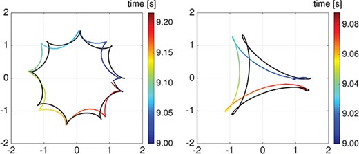
Sperm are navigating in a complex, 3D fluid environment in order to reach and penetrate the egg. Thus, it is necessary to study sperm motility in 3D (Guerrero et al., 2011). However, many experiments have analysed the motility of a few sperm where motility is recorded at a fixed depth. In this case, motility patterns observed were restricted in a given 2D plane. Recently, new technologies have been developed to trace the 3D trajectories of multiple sperm at the same time (Su et al., 2012, 2013; Jikeli et al., 2015). Observed sperm trajectories can vary from planar to quasi-planar, and to helical, possibly forming a chiral ribbon or a flagelloid curve (f-curve), as shown in Fig. 1 (Woolley & Vernon, 2001; Woolley, 2003; Smith et al., 2009a; Su et al., 2012, 2013). The particular trajectory observed depends on the species of sperm, on the proximity to the oviductal walls and on the external fluid properties. In particular, Smith et al. (2009a) and Woolley (2003) showed that the flagellar beat form can change from 3D to 2D as the fluid viscosity increases.
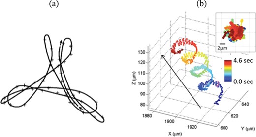
Experimental trajectories. (a) Trace of the midpiece of a mouse sperm swimming near a cover slip for a time period corresponding to 3.5 beats (approximately 0.35 seconds). (b) Trace of the head of a horse sperm for a time period of 4.6 seconds. The figures are reproduced, with permission, from Woolley (2003) and Su et al. (2013), respectively.
Different 2D and 3D elastohydrodynamic models have been developed to study flagellar motility and the interaction with the surrounding fluid, where the flagellum is either described at the continuum level (Gadêlha et al., 2010; Olson et al., 2011, 2013; Simons et al., 2014, 2015; Ishimoto & Gaffney, 2018), or at a more detailed level including the mathematical description of the discrete dynein motors, along with the accessory structures such as the microtubules and nexin links in the flagellum (Yang et al., 2008). In these models, the flagellar beat form is an emergent property. Another approach is to prescribe the flagellar beat form (Curtis et al., 2012; Ishimoto & Gaffney, 2016; Ishimoto et al., 2017). In all of these modelling studies, regardless of how the flagellar beat form is modelled, the observed sperm trajectory is an emergent property of the coupled system accounting for the fluid dynamics and the swimmer.
Only a few mathematical models have been developed to describe the time-dependent calcium dynamics within the sperm cell (Wennemuth et al., 2003; Olson et al., 2010; Li et al., 2014; Simons & Fauci, 2018). Wennemuth et al. (2003) studied in detail the calcium clearance phenomena along the flagellum via ATPase pumps. Later, Olson et al. (2010) developed a model that couples the ATPase pumps with the contributions of CatSper channels and a calcium store in the neck, motivated by experimental recordings of calcium fluorescence by Xia et al. (2007). Of the many modelling studies related to sperm motility, only a handful of models have attempted to consider the role of calcium dynamics on flagellar bending. Models have incorporated the effect of calcium indirectly by prescribing different waveforms for an activated (low calcium, symmetric waveform) or hyperactivated (high calcium, asymmetric waveform) sperm, without including any calcium dynamics directly in the model, to investigate emergent trajectories and interactions with a wall (Curtis et al., 2012; Olson & Fauci, 2015; Ishimoto & Gaffney, 2015, 2016). Another modelling approach has been to directly couple the sperm motility to either a temporal or spatiotemporal evolving calcium concentration via an asymmetric calcium-dependent curvature model where flagellar bending was planar (2D) (Olson et al., 2011; Olson, 2013; Simons et al., 2014). We remark that Olson et al. (2011) and Simons et al. (2014) explored both a spatiotemporal calcium coupling to a preferred beat form as well as a preferred beat form with a constant asymmetry. In these models, the evolving calcium dynamics were able to better match experimental data for emergent waveforms and trajectories. In the case of Simons et al. (2014), the direct calcium coupling to preferred amplitude also led to swimming trajectories that allowed escape from a planar wall, matching experimental observations of Chang & Suarez (2012). Thus, accounting for the relevant spatiotemporal evolution of calcium within the sperm flagellum is important to accurately model sperm motility.
Here, we develop the first mathematical model that couples the 3D dynamics of the sperm flagellum and the surrounding fluid, modelled respectively as a Kirchhoff rod and a Netwonian viscous fluid, with the CatSper channel-mediated calcium dynamics inside the flagellum, via a curvature-dependent coupling. The model is then used to investigate the emergent 3D waveforms and trajectories when coupling calcium and curvature, comparing to the 2D case. The planar bending case is fully characterized for the Kirchhoff rod model and compared to previous results when using an Euler elastica representation. Further, we investigate helical bending in the case of equal bending amplitudes (spiral bending) and the case of unequal bending amplitudes (quasi-planar since one amplitude is significantly smaller). The quasi-planar and helical bending cases exhibit emergent trajectories that can be described as a hypotrochoid, similar to the f-curve observed in experiments by Woolley (2003) (and reproduced in Fig. 1(a)).
2. Methods
2.1 Flagellum and fluid dynamics
Since we are interested in studying the motion of sperm in 3D, we utilize a Kirchhoff rod with preferred curvature and twist to model the elastic flagellum, as in Olson et al. (2013). As depicted in Fig. 2, the flagellum is represented by a 3D space curve |$\underline{\boldsymbol{X}}(t,s)$| and an associated orthonormal triad |$\{\underline{\boldsymbol{D}}^1(t,s),\underline{\boldsymbol{D}}^2(t,s),\underline{\boldsymbol{D}}^3(t,s) \}$| for |$0 \leqslant s \leqslant L$|, where |$L$| is the length of the unstressed rod, |$s$| is a Lagrangian parameter initialized as the arc length and |$t$| is time. The rod is assumed to have a circular cross section of constant radius that is much smaller than the rod length |$L$|.
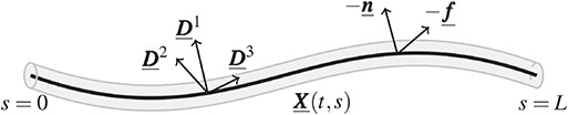
Sketch of the Kirchhoff rod model for the flagellum. The rod (grey) is represented by the space curve |$\underline{\boldsymbol{X}}(t,s)$| (thick black line) and an associated orthonormal triad |$\{\underline{\boldsymbol{D}}^1(t,s),\underline{\boldsymbol{D}}^2(t,s),\underline{\boldsymbol{D}}^3(t,s) \}$|, |$s$| is the rod spatial coordinate, |$L$| is the length of the unstressed rod and |$t$| is the temporal coordinate. |$\underline{\boldsymbol{f}}(t,s)$| and |$\underline{\boldsymbol{n}}(t,s)$| are the external force and torque per unit of length applied to the rod.
- The actual strain twist vector|$(\varOmega ^{\ast }_1,\varOmega ^{\ast }_2,\varOmega ^{\ast }_3)=\left (\frac{\partial \underline{\boldsymbol{D}}^2}{\partial s} \cdot \underline{\boldsymbol{D}}^3,\frac{\partial \underline{\boldsymbol{D}}^3}{\partial s} \cdot \underline{\boldsymbol{D}}^1,\frac{\partial \underline{\boldsymbol{D}}^1}{\partial s} \cdot \underline{\boldsymbol{D}}^{2}\right )$| is equal to the preferred strain twist vector|$(\varOmega _1,\varOmega _2,\varOmega _3)$|; hence, the actual curvatureis equal to the preferred curvature|$\varOmega $| in (2.2).(2.7)$$\begin{equation} \varOmega^{\ast}=\sqrt{\left(\varOmega^{\ast}_1\right)^2 + \left(\varOmega^{\ast}_{2}\right)^{2}}=\sqrt{\left(\frac{\partial \underline{\boldsymbol{D}}^2}{\partial s} \cdot \underline{\boldsymbol{D}}^{3}\right)^{2} + \left(\frac{\partial \underline{\boldsymbol{D}}^3}{\partial{s}}\cdot \underline{\boldsymbol{D}}^{1}\right)^{2}} \end{equation}$$
|$\underline{\boldsymbol{D}}^3$| is aligned with the tangent vector, both |$\underline{\boldsymbol{D}}^1$| and |$\underline{\boldsymbol{D}}^2$| are orthogonal to the tangent vector and the rod is inextensible, i.e |$\left |\frac{\partial{\underline{\boldsymbol{X}}}}{\partial{s}}\right | =1$|.
The material and geometric parameters of the sperm flagellum, the calcium model parameters, as well as the numerical algorithm parameters.
The material and geometric parameters of the sperm flagellum, the calcium model parameters, as well as the numerical algorithm parameters.
Accordingly, at each instant in time, given the force exerted by the rod on the fluid, we can solve for the resulting fluid flow and update the rod location assuming it moves with the local fluid velocity.
2.2 Calcium and curvature dynamics
In mammalian sperm, the asymmetry and magnitude of flagellar bending is known to vary as a function of the calcium concentration inside the flagellum (Tash & Means, 1982; Lindemann & Goltz, 1988; Ho & Suarez, 2001b; Ho et al., 2002; Marquez & Suarez, 2007b; ). We will use a previously developed 1D reaction–diffusion model to account for the relevant calcium dynamics (Olson et al., 2010). The increase in intracellular calcium concentration is initiated by the opening of CatSper channels (Carlson et al., 2003; Xia et al., 2007), which allows calcium to flow from the external fluid bath to the inside of the sperm flagellum. The sperm is composed of five pieces: the head, neck, mid-piece, principal piece and end piece (Cummins & Woodall, 1985; Pesch & Bergmann, 2006). Channels such as CatSper (Chung et al., 2014) and pumps such as the calcium ATPase pump (Okunade et al., 2004) are localized along the length of the principal piece, whereas the redundant nuclear envelope (RNE), a calcium store (Ho & Suarez, 2001a, 2003), is found in the neck.
Figure 3(a) shows the calcium dynamics in time for the case of a fixed straight rod (i.e. |$\left |\partial \underline{\boldsymbol{X}}(t,s)/{\partial s}\right |=1$|) at three different points along the sperm length |$L$|: N - at |$1\% \ \textrm{of} \ L $|, MP - at |$16\%$| of |$L$| and PP - at |$24\%$| of |$L$|. The locations of the points N, MP and PP have been chosen to illustrate calcium entry through CatSper channels in the principal piece at earlier time points, calcium-induced calcium release in the neck at later time points and an increase in calcium in the mid-piece and principal piece due to diffusion along the length of the flagellum. Note that these calcium trends match the calcium fluorescence results of Xia et al. (2007). Additionally, we have utilized the model in Olson et al. (2010) where we have only updated the scaling of the flagellum to be characteristic of human sperm, as reported in Table 1, and we are now neglecting the head region in this work (in contrast to Olson et al., 2010).
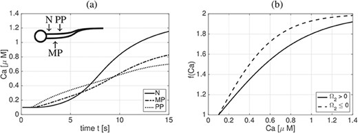
Calcium dynamics. (a) Calcium (|$Ca$|) concentration dynamics in time for the case of a fixed, straight rod at three different points along the sperm length |$L$|: N at |$1\%$| of |$L$|, MP at |$16\%$| of |$L$|, and PP at |$24\%$| of |$L$|. (b) Plot of |$f$|, given in (2.16), as a function of calcium concentration |$Ca$| depending on the sign of the preferred normal curvature |$\varOmega _2$|.
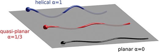
Flagellar beat forms. Schematic representation of the three flagellar beat forms considered: planar wave (bottom), quasi-planar wave (middle) and helical wave (top), and their corresponding value of the chirality parameter |$\alpha $|.
2.3 Numerical algorithm for coupling
At time |$t=0$|, the rod and orthonormal triads are initialized using the preferred reference configuration in (2.14) for a given set of wave parameters and the rod is discretized into |$M+1$| points with constant spacing |$\triangle s=L/M$|, i.e. |$s_k=k \triangle s$| for |$k=0,\ldots ,M$| (additional details given in Appendix A). The following steps are followed to solve for the new configuration of the rod at time |$\triangle t$|.
Compute the calcium concentration along the rod by solving (2.13) as in Olson et al. (2010, 2011). A symmetric Crank–Nicolson scheme detailed in Lai et al. (2008) is used, which ensures that the total mass of calcium is numerically conserved in the case of flux |$J=0$|;
Given the calcium concentration, determine the preferred amplitude in (2.15) for |$A$| and |$B$| at each discretized point along the rod;
Determine the preferred strain and twist |$\Omega _i$| in (2.17) for each of the |$M+1$| points, assuming |$A$| and |$B$| constant at each point;
Calculate the point forces |$\underline{\boldsymbol{f}}_k$| and torques |$\underline{\boldsymbol{n}}_k$| along the rod using (2.3)–(2.6) as in Olson et al. (2013);
- Solve for the fluid flow in (2.8) and (2.9) using regularized fundamental solutions; the local linear velocity |$\underline{\boldsymbol{v}}$| and angular velocity |$\underline{\boldsymbol{w}}$| are given as(2.20)$$\begin{align} \underline{\boldsymbol{v}}(\underline{\boldsymbol{x}})&=\frac{1}{\mu}\sum_{k=0}^{M}\mathscr{S}[-\underline{\boldsymbol{f}}_k\triangle s]+\frac{1}{\mu}\sum_{k=0}^{M}\mathscr{R}[-\underline{\boldsymbol{n}}_{k}{\triangle} s], \end{align}$$where |$\mathscr{R}$|, |$\mathscr{S}$| and |$\mathscr{D}$| are the regularized rotlet, Stokeslet and dipole for the blob function given in (2.10), as detailed in Olson et al. (2013);(2.21)$$\begin{align} \underline{\boldsymbol{w}}(\underline{\boldsymbol{x}})&=\frac{1}{2}\nabla\times\underline{\boldsymbol{v}}=\frac{1}{\mu}\sum_{k=0}^{M}\mathscr{R}(-\underline{\boldsymbol{f}}_k\triangle s)+\frac{1}{\mu}\sum_{k=0}^{M}\mathscr{D}(-\underline{\boldsymbol{n}}_k\triangle s), \end{align}$$
Update the rod location |$\underline{\boldsymbol{X}}$| and orthonormal triads |$\underline{\boldsymbol{D}}^i$| for |$i=1,2,3$| using the local linear and angular velocity via the no-slip conditions in (2.12). The forward Euler method is used to solve these equations.
3. Results and discussion
We investigate the effect of the calcium and curvature coupling described in Section 2.2 on sperm motility. The flagellar beat forms we consider are illustrated in Fig. 4 and are given as follows:
2D dynamics: planar wave with |$A_0=3$||$\mu $|m and |$B_0=0$||$\mu $|m, i.e. |$\alpha =0$|;
3D dynamics:
i)helical wave with |$A_0=B_0=3$||$\mu $|m, i.e. |$\alpha =1$|;
ii)quasi-planar wave with |$A_0=3$||$\mu $|m and |$B_0=1$||$\mu $|m, i.e. |$\alpha =1/3$|.
a) no-coupling (No Ca): |$A$| and |$B$| are fixed to the baseline values, i.e. |$A=A_0$| and |$B=B_0$|;
b) symmetric coupling (Ca sym): |$A$| and |$B$| vary symmetrically with respect to curvature, i.e. in (2.16) |$c_2=c_{2,p}=c_{2,n}=1\mu $|M;
c) asymmetric coupling (Ca asym|$A$|&|$B$|): |$A$| and |$B$| vary asymmetrically with respect to curvature, i.e. in (2.16) |$c_{2,p}\neq c_{2,n}$| as in Table 1;
d) asymmetric coupling only A (Ca asym|$A$|): |$A$| varies asymmetrically with respect to curvature, while |$B$| is kept constant to its baseline value, i.e. |$B=B_0$|.
The material and geometric parameters of the sperm flagellum, as well as the calcium model parameters, are summarized in Table 1, with references given where applicable. In particular, the flagellar beat form parameters |$L$|, |$A_0$|, |$B_0$|, |$\sigma $| and |$k$|, reported in Table 1, have been taken directly from the reported references. The values for the different regions of the flagellum are reported in Table 1. These ranges are based on the average dimensions of the mammalian sperm flagellum reported in Cummins & Woodall (1985) and Pesch & Bergmann (2006), following the same proportions between region size and flagellum size used in Olson et al. (2010) and accounting for the fact that in this model, in contrast to Olson et al. (2010), we are neglecting a sperm head region. The values for the material properties of a mammalian sperm flagellum, i.e. |$a_i$| and |$b_i$|, have been determined by starting from the shear and bending resistance values extracted from sea urchin sperm in Pelle et al. (2009) and Okuno & Hiramoto (1979). These were adjusted by one or two orders of magnitude to take into account the fact that mammalian sperm are generally stiffer than invertebrate sperm due to the presence of the outer dense fibres (Lindemann et al., 1973; Schmitz & Lindemann, 2004; Zhao et al., 2018). The values of |$D_{Ca}$| and |$\widehat{Ca}$| have been taken directly from the reported references, in accordance to Olson et al. (2010), while the values of |$c_1$|, |$c_{2,p}$| and |$c_{2,n}$| have been chosen phenomenologically. For example, |$c_1$| is chosen so that the function |$f(Ca)$|, depicted in Fig. 3(b), attains |$90\%$| of its upper bound for |$Ca=c_2$|. Considering that the calcium dynamics, reported in Fig. 3(a), are fully developed after |$t=10$|s, we choose |$c_{2,n}=1\mu $|M, and |$c_{2,p}=0.7\mu $|M|$<c_{2,n}$| to introduce the bending asymmetry by means of changing the slope of the function |$f$|.
The values for the numerical algorithm parameters are also listed in Table 1 and were chosen to ensure convergence and stability of computational results. In particular, the value of the regularization parameter |$\varepsilon $| is chosen to comply to its physical and numerical interpretation. We note that the singular Stokeslet solution is obtained in the limit as |$\varepsilon \to 0$| and the magnitude of |$\varepsilon $| will in turn control the regularization error. Thus, we want to minimize error but still have a physically accurate representation of the flagellum since, via the blob function (2.10), |$\varepsilon $| also represents the radius of the spherical region around a point where the majority of the force or torque is spread to the fluid (Cortez et al., 2005). This is why we can also view |$\varepsilon $| as a physical parameter: the virtual radius of the flagellar cross section. We chose |$\varepsilon =1\mu $|m in agreement with the characteristic radii for the mid-piece of mammalian sperm reported in Cummins & Woodall (1985). Moreover, in order for the derivation of force and torque balance on the Kirchhoff rod to be valid, we must have that the rod radius is much smaller than the length, and this is satisfied with the reported virtual rod radius |$\varepsilon $| and rod length |$L$|. The proportionality between |$\triangle s$| and |$\varepsilon $| is chosen to make sure that the blob functions overlap sufficiently and to ensure that the fluid does not leak through the rod centreline (Cortez, 2018). The value of |$\triangle t$| is chosen small enough to ensure numerical stability of the forward Euler method used for the time discretization (Olson et al., 2013).
In this section, we omit results for calcium concentration dynamics along the flagellum since they are analogous to the case of a fixed rod shown in Fig. 3(a), with the minor addition of infinitesimal oscillations due to the deformation of the rod, see Olson et al. (2011) for more details.
3.1 2D flagellar dynamics
Figure 5 shows sperm trajectories over a 15-second interval for simulations corresponding to the different cases of calcium-curvature coupling. Note that in the planar wave case |$\varOmega _1=\varOmega _3=0$| since |$B=0$|; hence, the preferred curvature of the rod is |$\varOmega =|\varOmega _2|$|. For this curvature case, in both the symmetric and asymmetric coupling cases, we observe that the sperm has a higher linear velocity (|$\mu $|m s|$^{-1}$|) compared to the no-coupling case: No Ca - |$28.9$|, Ca sym - 40.4 and Ca asym - |$34.9$|. The linear velocities extracted from the model results are in agreement with the experimental measurements for human sperm reported in Smith et al. (2009a). However, the Ca sym is not enough to reproduce the calcium-dependent turn in the sperm trajectory observed in vivo (Marquez & Suarez, 2007a). Only when the beat asymmetry is included in the coupling, the numerical results are able to reproduce the turning phenomenon. This is similar to previous computational results for a 2D model of a sperm using an Euler elastica representation of the flagellum (Olson et al., 2011). For this reason, we will only consider the asymmetric coupling cases in the rest of the results section. In the case of asymmetric calcium coupling, we remark that the trajectory starts as straight but as the calcium increases in the principal piece due to CatSper channels opening, this initiates calcium-induced calcium release in the neck region, which then causes an increase in calcium along the length of the flagellum due to diffusion (Fig. 3(a)). In Fig. 5, the increased path curvature due to the turning motion starts at |$t=5$|s when the calcium is increasing and reaches a stable trajectory for |$t=10-15$|s when calcium is reaching maximal values along the flagellum.
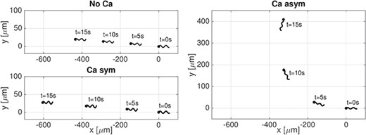
Planar wave. Sperm trajectories in time |$t$| from 0 to |$15$|s for the case of No Ca, Ca sym, and Ca asym. A filled in circle is used to denote the first point of the flagellum in the direction of swimming.
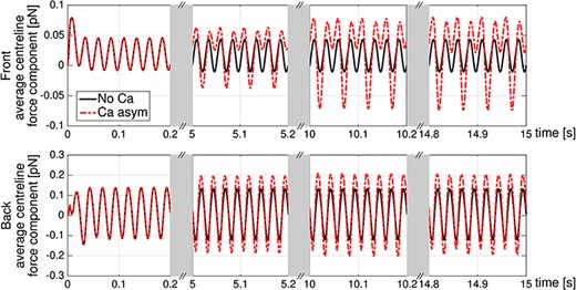
Planar wave. Average centreline force component |$f_{\textit{c}}(t,s)$| in the front region of the rod (first |$20$| points of the spatial discretization, top panel) and in the back region of the rod (last |$20$| points of the spatial discretization, bottom panel) for no-coupling (No Ca, solid line) and asymmetric coupling (Ca asym, dashed line) cases. For |$t=0$| to |$0.2$|s, the curves lie on top of each other.
In Figs 7 and 8 we investigate the effect of varying the flagellum material properties on the motion of the sperm. We can consider the moduli |$a_i$| as both numerical and material parameters. As numerical parameters, the moduli are Lagrange multipliers that enforce how strictly the curvature and twist are enforced. In addition, these moduli give an effective stiffness to the elastic rod that represents the sperm flagellum. From experiments, we know that the stiffness varies by several orders of magnitude for different species of sperm, where mammalian sperm are generally stiffer than invertebrate sperm (Lindemann et al., 1973; Schmitz & Lindemann, 2004; Pelle et al., 2009). Thus, we run simulations where the bending and twist moduli |$a_i$|, in Table 1, have been reduced by a factor of |$5$| and by a factor of |$10$|. In this parameter regime, the larger bending and twist moduli correspond to a stiffer elastic rod, i.e. stiffer microtubules and outer dense fibres of the flagellum. We remark that in these simulations the radius of the rod cross section is kept constant, i.e. |$\varepsilon $| is kept constant. Figure 7 shows the trace of the flagellum first point in the direction of swimming over 15 seconds in the case of No Ca (left) and in the case of Ca asym (right) for the three bending and twist moduli values considered. For this range of material properties considered, the rod first point shows, in general, a linear trajectory in the No Ca case and a clockwise turning trajectory in the Ca asym case. Moreover, in the Ca asym case, the trajectory radius of curvature is directly proportional to the bending and twist moduli, and the linear speed is also proportional to |$a_i$| in both coupling cases considered. While the rod first point trace shows a general linear or turning trajectory, in reality, as shown in the zoomed area of Fig. 7, the rod first point trace is an oscillating curve in time. The amplitude and frequency of these oscillations vary with the material properties and the coupling condition considered, while the shape of the oscillations vary with the material properties but seem to be independent from the coupling condition.
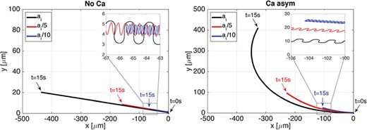
Planar wave. Trajectories of the flagellum first point in the direction of swimming in time |$t$| varying the bending and twist moduli |$a_i$|: moduli as in Table 1 (largest sperm progression), reduced by a factor of |$5$| (moderate sperm progression) and reduced by a factor of |$10$| (smallest sperm progression). No Ca case is on the left and Ca asym case is on the right. The zoomed in portion highlights that the trajectories oscillate in time.
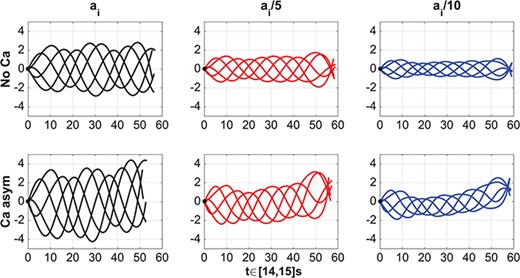
Planar wave. Evolution of flagellum (translated and rotated to the horizontal axis) for |$t=14$|s to |$15$|s, spatial units shown are in microns. No-coupling (No Ca, top row), asymmetric coupling (Ca asym, bottom row), bending and twist moduli as in Table 1 (left), moduli reduced by a factor of |$5$| (centre) and moduli reduced by a factor of |$10$| (right). The black circle at the origin denotes the first point on the flagellum.
In Fig. 8, the flagellar configurations are illustrated for different values of bending and twist moduli |$a_i$|, over the time interval |$14$| to |$15$|s. The configurations are translated and rotated so that the rod first point in the direction of swimming is at the origin and the centreline lies on the horizontal axis, where spatial units are shown in microns. Each row corresponds to a calcium-curvature coupling case, and each column corresponds to different flagellum material properties. The results show that the emergent flagellar wave amplitude, for this range of moduli and preferred beat form parameters, decreases as bending and twisting moduli are decreased. The largest amplitude achieved corresponds to the preferred amplitude. Since the emergent amplitude is partially determined by the flagellum trying to minimize the energy given in (2.1), the amplitude achieved along the length is non-constant and, as in Fig. 8, tends to increase from the first point in the direction of swimming to the last point. For all the values of bending and twist moduli considered, there is an increase in the wave amplitude when the asymmetric coupling is considered, and this increase is proportional to the corresponding no-coupling configuration. Moreover, the Ca asym generates an increased tilt of the end piece with respect to the centreline, and this phenomenon is more prominent as the bending and twisting moduli decrease. We also note that trajectories and observed waveforms for varying moduli in the Kirchhoff rod model are similar to those for an Euler elastica model (Olson et al., 2011).
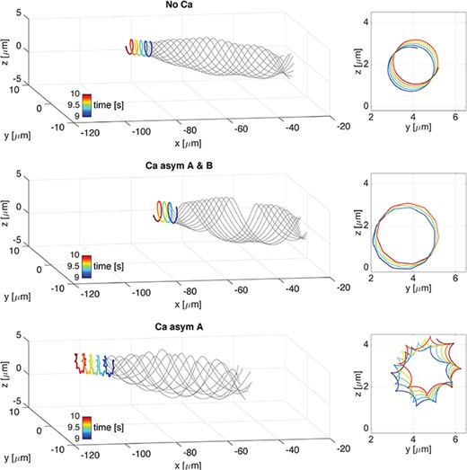
Helical wave. 3D overlap of flagellar configurations (thin grey lines) and the trajectory of the first point in the direction of swimming (thick coloured line) over the time interval of |$1$|s, from |$9$| to |$10$|s, on the left. Corresponding f-curve traced by the first point on the |$yz$|-plane, on the right. Cases are: No Ca (top), Ca asym A & B (centre), and Ca asym A (bottom). Note that the head trace shifts upwards in z and to the right in y as time progresses.
3.2 3D dynamics
3.2.1 Helical wave
In the helical wave case, Fig. 9 shows the overlap of flagellar configurations (thin grey lines) and the trajectory of the first point in the direction of swimming (thick coloured line) over the time interval of |$1$|s, from |$9$| to |$10$|s, for three different coupling cases: No Ca, Ca asym|$A$|&|$B$| and Ca asym|$A$|. On the right is depicted the corresponding f-curve traced by the first point on the |$yz$|-plane. The f-curve is defined as the path followed by a fixed point on the flagellum (Woolley, 1998). In the No Ca and Ca asym|$A$|&|$B$| coupling cases, the flagellar configurations remain helical in time, with increased amplitudes in the Ca asym|$A$|&|$B$| case, and the f-curves traced by the first point are almost circular. In the Ca asym|$A$| coupling case, the flagellar configurations show an irregular beat pattern and the first point f-curve resembles a hypotrochoid with eight singular points, with increased amplitudes in comparison to the No Ca case. We note that the linear velocity of the Ca asym|$A$|&|$B$| case is |$12\%$| lower than the No Ca case, see Table 3, due to the higher amplitude and almost perfect helical shape, i.e. chirality parameter |$\alpha \simeq 1$|. While, in the Ca asym|$A$| case, the irregularity of the flagellum shape together with the increase in wave amplitudes produces an increase of |$53\%$| in the linear velocity compared to the No Ca case, see Table 3.
Variations in the actual curvature |$\Omega ^{\ast }$| (2.7) along the flagellum spatial coordinate |$s$| in the time interval from |$9$| to |$9.2$|s are reported in Fig. 10, for the same three coupling cases investigated in Fig. 9. In the No Ca and Ca asym|$A$|&|$B$| coupling cases the flagellum curvature is almost constant, and this is consistent with the helical flagellum configuration reported in Fig. 9, since helices by definition have constant curvature and twist. However, in the Ca asym|$A$| case the curvature varies periodically along the flagellum, and this is consistent with the irregular flagellum beating reported in Fig. 9. In all three coupling cases, the normalized absolute difference between the actual curvature |$\varOmega ^{\ast }$| and the preferred curvature |$\varOmega $| (2.2) is less than |$1\times 10^{-2}$|.
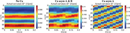
Helical wave. Actual curvature |$\Omega ^{\ast }$| variations along the flagellum spatial coordinate |$s$| in the time interval from |$9$| to |$9.2$|s. Cases are: No Ca (left), Ca asym A & B (centre), and Ca asym A (right).
3.2.2 Quasi-planar wave
In the case of a quasi-planar wave propagating along the flagellum, Fig. 11 shows flagellar configurations (thin grey lines) and the trajectory of the first point in the direction of swimming (thick coloured line) over the time interval of |$1$|s, from |$9$| to |$10$|s. The three different coupling cases considered are No Ca, Ca asym|$A$|&|$B$| and Ca asym|$A$|. On the right is depicted the corresponding f-curve traced by the rod first point on the |$yz$|-plane. In all of the coupling cases, the flagellum configuration shows an irregular beat form, due to the baseline geometric non-linearity introduced by the quasi-planer wave, i.e |$A_0\neq B_0$|. At the same time, the three cases differ from each other in terms of the emergent shapes of the first point f-curve, achieved wave amplitude, and linear velocity. In the No Ca and Ca asym|$A$|&|$B$| cases, the first point f-curves resemble a hypotrochoid with four singular points, while in the Ca asym|$A$| case, the first point f-curves resemble a hypotrochoid with three singular points. Moreover, the two asymmetric coupling cases show visible increased amplitudes in comparison to the No Ca case. The linear velocity of the quasi-planar wave cases are reported in Table 3. The Ca asym|$A$|&|$B$| and Ca asym|$A$| couplings produce an increase in the linear velocity of |$37\%$| and |$76\%$| compared to the no-coupling case, respectively.
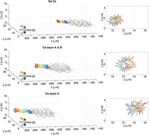
Quasi-planar wave. 3D overlap of flagellar wave (thin grey lines) and the trajectory of the first point in the direction of swimming (thick coloured line) over the time interval of 1s, from 9 to 10s, on the left. Corresponding f-curve traced by the first point on the |$yz$|-plane, on the right. Cases are: No Ca (top), Ca asym A & B (centre), and Ca asym A (bottom). Note that the head trace shifts upwards in z and to the right in y as time progresses.
In the quasi-planar case, for all three coupling cases considered in Fig. 11, the curvature is not constant along the flagellum length and periodically oscillates in time. In particular, Fig. 12 shows the comparison between preferred curvature |$\varOmega $| (2.2) and preferred twist |$\varOmega _3$| (solid lines) with the actual curvature |${\varOmega }^{\ast }$| (2.7) and actual twist |$\varOmega _3^{\ast }$| (dashed lines), for the No Ca and the Ca asym|$A$| cases, at time |$t=10s$|. The maximum curvature and twist in the Ca asym|$A$| is almost twice that of the No Ca case, and both cases present a phase lag between the oscillations of the preferred and computed curvature and twist.
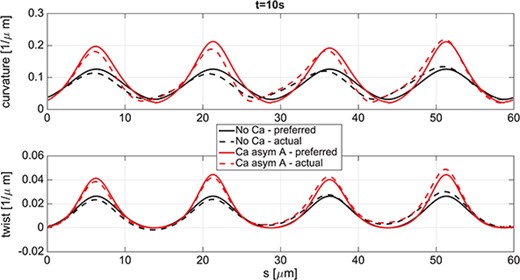
Quasi-planar wave. Comparison at |$t=10$|s between preferred (solid lines) and actual (dashed lines) configurations of the rod; curvature in the top panel and twist in the bottom panel for the case of No Ca (curves with smaller local maxima) and in the case of Ca asym A (curves with larger local maxima).
3.2.3 Hypotrochoid approximation of rod first point f-curves
Helical vs quasi-planar waves. Comparison between simulation results for a full rotation of the rod first point f-curve around the centre of mass (coloured line) and the corresponding fitted hypotrochoid curve (black line) for the case of a helical wave (left) and a quasi-planar wave (right), considering the Ca asym A case.
The fitted hypotrochoid parameter values varying the flagellar waveform and varying the calcium-curvature coupling condition: No Ca, Ca asym A & B, and Ca asym A.
| Wave | Coupling case | |$\widetilde{R}$| [|$\mu $|m] | |$d$| [|$\mu $|m] | |$\omega _1$|[rad/s] | |$\omega _2$|[rad/s] | |$n$| |
|---|---|---|---|---|---|---|
| No Ca | |$1.091$| | |$0.003$| | |$29.7$| | |$29.7$| | |$2.0^{a}$| | |
| Helical | Ca asym A & B | |$1.451$| | |$0.019$| | |$20.3$| | |$215.6$| | |$11.6$| |
| Ca asym A | |$1.272$| | |$0.180$| | |$28.5$| | |$210.5$| | |$8.4$| | |
| No Ca | |$0.796$| | |$0.297$| | |$ 62.5$| | |$169.0$| | |$3.7$| | |
| Quasi-planar | Ca asym A & B | |$1.049$| | |$0.375$| | |$51.6$| | |$172.2$| | |$4.3$| |
| Ca asym A | |$0.945$| | |$0.510$| | |$68.5$| | |$145.9$| | |$3.1$| |
aValue imposed a priori in order to obtain a circle.
Comparison of rod first point linear velocity, maximum curvature and maximum distance form the centreline for the various flagellar wave and calcium-curvature coupling conditions: No Ca, Ca asym A & B, and Ca asym A.
| Coupling case | Linear velocity [|$\mu $|ms|$^{-1}$|] | Max. curvature [1/|$\mu $|m] | Max. distance [|$\mu $|m] | |||
|---|---|---|---|---|---|---|
| Helical | Quasi-planar | Helical | Quasi-planar | Helical | Quasi-planar | |
| No Ca | |$8.6$| | |$22.1$| | |$0.09$| | |$0.13$| | |$2.86$| | |$2.87$| |
| |$Ca\ asym\ A$| & |$B$| | |$7.6$| | |$30.4$| | |$0.11$| | |$0.20$| | |$3.94$| | |$3.91$| |
| |$Ca\ asym\ A$| | |$13.2$| | |$38.9$| | |$0.16$| | |$0.22$| | |$3.82$| | |$3.95$| |
To better quantify the various f-curve shapes reported in Figs 9 and 11, we follow the method reported in Woolley (1998) to approximate the f-curve via a hypotrochoid curve, and the results of the approximation are reported in Fig. 13 and in Table 2. More details on the approximation procedure can be found in Appendix B. Figure 13 shows the comparison between the simulation results for one full rotation of the f-curve (coloured curve) and the approximated hypotrochoid curve (black curve) in the case of a helical wave (left), and of a quasi-planar wave (right), considering the Ca asym A. In Table 2, we report the fitted parameter values for the hypotrochoid in the case of helical and quasi-planar waves and, for the three curvature-calcium coupling cases considered in Figs 9 and 11. In the two wave configurations studied, both calcium coupling cases considered produce an increase in the radius |$\widetilde{R}$| compared to the non-coupling case, while showing different hypotrochoid shapes. In particular, in the Ca Asym A&B case, |$\widetilde{R}$| is about |$30\%$| higher than the no-coupling case while maintaining a similar hypotrochoid shape; a circular shape for the helical wave case (|$d\simeq 0$|) and a square shape (|$n\simeq 4$|) for the quasi-planar wave case. However, in the Ca Asym|$A$| case, compared to the no-coupling case, |$\widetilde{R}$| is only about |$15\%$| higher, but the hypotrochoid shape varies from a circular (|$n=2$|) to an octagonal shape (|$n\simeq 8$|) in the helical wave case and from a square (|$n\simeq 4$|) to a triangular shape (|$n\simeq 3$|) in the quasi-planar wave case. The shapes of the hypotrochoid f-curves extracted from the model results are in agreement with the experimental measurements reported in Woolley (1998, 2003) and Woolley & Vernon (2001) and reproduced in Fig. 1(a). In the model results, the left-handedness of the rod trajectories, given by the rod preferred reference configuration (2.14), causes a predominant counterclockwise sperm rolling motion, i.e. a predominant counterclockwise rotation of the f-curves reported in Figs 9 and 11. Moreover, the counter rotation (clockwise) of the flagellum is significantly present only if a difference between the preferred amplitudes |$A$| and |$B$| is introduced. In our model, |$A\neq B$| can be obtained in two ways: a baseline geometrical difference in the quasi-planar wave case where |$A_0\neq B_0$|, and a calcium coupling difference in the Ca Asym|$A$| case, where only |$A$| varies with calcium and |$B$| is kept constant to its baseline value.
3.2.4 Comparison of helical & quasi-planar waves
To investigate the fluid–structure interaction between the flagellum and the surrounding fluid, in Fig. 14 we report the fluid velocity fields (black arrows) and pressure (|$p$|) distributions at time |$t=10$|s. We choose either a horizontal or vertical plane containing the flagellum centreline in the case of helical and quasi-planar waves, accounting for the Ca asym|$A$| coupling. The horizontal centreline plane is defined as the plane passing through the sperm centreline with normal orthogonal to the |$y$|-axis, while the vertical centreline plane is defined as the plane passing through the sperm centreline with normal orthogonal to the |$z$|-axis. The pressure distribution range is approximately |$-40$| to |$40$| g|$\mu $|ms|$^{-2}$| in the helical wave case, and from |$-80$| to |$80$| g|$\mu $|ms|$^{-2}$| in the quasi-planar wave case. In both wave cases, the velocity fields show vortices along the flagellum length, where the fluid rotates from regions of negative pressure to regions of positive pressure.
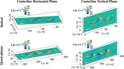
Helical vs quasi-planar waves. Fluid velocity fields (black arrows) and pressure (|$p$|) distributions at time |$t=10$|s in the flagellum horizontal (left column) or vertical (right column) centreline planes in the case of a helical wave (top row) and a quasi-planar wave (bottom row), for the Ca asym A case. A filled in sphere is used to denote the rod first point and a white arrow to denote the swimming direction.
In Table 3, we report the values of the linear velocity of the rod first point in the direction of swimming, rod maximum actual curvature |$\varOmega ^{\ast }$|, and rod maximum distance from the centreline over the |$1$|s interval from |$9$| to |$10$|s in the case of No Ca, Ca asym A & B, and Ca asym A, for the helical and quasi-planar waves. In both wave configurations, the Ca asym|$A$| coupling produces the highest velocities and highest curvatures. Note that the linear velocities and maximum curvatures in the quasi-planar wave case are significantly higher than the helical case: from |$2.6$| to |$4$| times higher for velocities, and from |$1.3$| to |$1.8$| times higher for curvatures. The maximum distance shows a non-linear behaviour as the waveform changes and as the calcium-curvature coupling condition changes. The maximum distance increases approximately |$35\%$| in the Ca asym|$A$|&|$B$| coupling case compared to the no-coupling case, and there is no significant variation in the Ca asym|$A$| coupling case compared to the Ca asym|$A$|&|$B$| coupling case. There is no significant difference in the maximum distance values between the helical and the quasi-planar cases, independently from the calcium-curvature coupling considered. Most previous models have indirectly accounted for calcium via a prescribed flagellar beat form and hence we can not compare our emergent amplitudes to these cases. In comparison to models of 2D flagellar bending where calcium dynamics were directly coupled, a non-monotonic behaviour in achieved amplitude has also been observed and shown qualitatively in graphs of the flagellar beat form (Olson et al., 2011; Simons et al., 2014).
In Fig. 15, the f-curves traced by the end point of the tail on the |$yz$|-plane are reported over three |$1$|s time intervals: from |$4$| to |$5$|s (left column), from |$9$| to |$10$|s (middle column) and from |$14$| to |$15$|s (right column). The helical wave case is reported on the top row and the quasi-planar wave case is on the bottom row, accounting for the Ca asym|$A$| coupling. We observe that the tail f-curves show a similar shape to the f-curves reported in Figs 9 and 11, namely hypotrochoids with eight singular points for the helical wave, Ca asym|$A$| case, and hypotrochoids with three singular points for the quasi-planar wave, Ca asym|$A$| case. Hence, the results show that the f-curve shape travels along the flagellum length and is conserved in the tail f-curve.
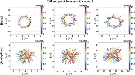
Helical vs Quasi-planar waves. Tail end point f-curves on the |$yz$|-plane over three time intervals of |$1$|s (left column: from |$4$| to |$5$|s, middle column: from |$9$| to |$10$|s, right column: from |$14$| to |$15$|s) in the case of a helical wave (top row) and a quasi-planar wave (bottom row), for the Ca asym A case. As time progresses, the f-curves are increasing in both z and y.
4. Conclusions
This paper presents the first mathematical model that couples the 3D dynamics of the sperm flagellum and surrounding fluid, with the calcium dynamics inside the flagellum. The coupling is achieved by assuming that the preferred curvature and twist of the flagellum depends on the local calcium concentration. We compare the model results for 2D and 3D flagellar reference beat forms: planar, helical and quasi-planar. Linear velocities, forces and trajectories extracted from the model results are in agreement with experimental data and previously developed mathematical models (Smith et al., 2009a; Woolley, 1998; Woolley & Vernon, 2001; Woolley, 2003; Olson et al., 2011; Simons et al., 2014).
In particular, the planar swimmer results reveal that (i) turning motion on the time scale of seconds is obtained only when asymmetric calcium coupling is considered and (ii) a significantly higher linear velocity is obtained relative to the helical swimmer, in agreement with Chwang & Wu (1971). These model results support the hypothesis that helical motion might be an important strategy for chemotaxis sampling. Chemotaxis is defined as the movement towards a chemical concentration gradient such as an egg protein in marine invertebrate sperm or progesterone in human sperm (Wood et al., 2005; Lishko et al., 2011). Swimming with a helical beat form could potentially help the sperm to slow down and sample a larger area, which might aid in the determination of the direction corresponding to an increase in the chemoattractant (Guerrero et al., 2011; Su et al., 2013, 2012). In the case of 3D flagellar beat forms, if an asymmetry between the amplitudes |$A$| and |$B$| is introduced (corresponding to a chirality parameter |$0<\alpha <1$| for |$A=\alpha B$|), the f-curves extracted from the model resemble hypotrochoid curves. In this paper we investigate two sources of asymmetry: a geometrical asymmetry in the quasi-planar wave case and a calcium coupling asymmetry in the Ca Asym A case. The shape of the hypotrochoid f-curve, i.e. the number |$n$| and the presence or absence of cusps and self intersections, varies with the choice of preferred flagellar amplitudes |$A_0$| and |$B_0$|, and with the calcium coupling considered. However, the shape of the f-curve is maintained along the length of the flagellum in each case considered. We remark that hypotrochoid f-curves similar to the one extracted from the model results have been obtained in the experimental measurements reported by Woolley (1998, 2003) and theoretical predictions reported by Smith et al. (2009b) and Ishimoto & Gaffney (2018).
Throughout the development of the model, several assumptions were made. We utilized a simplified sperm representation which neglected the cell body or head. Experiments have shown that headless mammalian sperm can still swim in fluid flows (Miki & Clapham, 2013). Moreover, since the head is small compared to the length scale of the flagellum, a dimensional analysis by Ishimoto & Gaffney (2015) showed that neglecting the head still results in an angular and linear velocity of the correct scale. Therefore, accounting for the head in the model should not significantly affect the overall sperm motility. Further studies are required to investigate the head effect on sperm trajectories and f-curves since the presence of the cell body will certainly increase the drag and potentially bias trajectories and/or turning behaviour. In addition, we have used Stokes equations for the fluid flow and all results can be interpreted for the case of a homogeneous fluid with the same viscosity of water. Hence, we have ignored non-Newtonian or resistive effects due to polymers or proteins that are often found in oviductal or vaginal fluid (Rutllant et al., 2005; Miki & Clapham, 2013), as well as polyacrylamide or methylcellulose gels used in experiments (Suarez & Dai, 1992; Woolley, 2003; Smith et al., 2009a). We note that experimental observations where the flagellar beat form varies from 3D to 2D as viscosity varies (Woolley, 2003; Smith et al., 2009a) are not captured in this model, but this will be the focus of future modelling studies using more complicated fluid models.
In this work, we have focused on constant beat form parameters and material parameters (moduli |$a_i$| and |$b_i$|) in a physiologically representative range (see references in Table 1). The emergent beat form and trajectory are achieved due to a combination of the preferred beat form parameters, material parameters, as well as contributions from the viscous fluid (via the no-slip condition). For a preferred symmetric beat form, we observe linear trajectories where there is a slight tilt or yaw in the upward direction (increasing in |$y$| for the planar case, Fig. 7, and increasing in both |$y$| and |$z$| for the quasi-planar and helical cases, Figs 9 and 11), similar to previous models (Gillies et al., 2009; Smith et al., 2009b; Olson et al., 2011; Simons et al., 2014). We note that the emergent flagellar dynamics might exhibit behaviour deviating far from the preferred curvature (e.g. buckling instability as in Lee et al., 2014 and Park et al.2017) for a different range of parameters or in the case of anisotropies in material or geometric parameters. To simplify the representation of the flagellum, we have considered an isotropic rod and neglected the fact that the sperm flagellum has a non-constant cross-sectional radius and non-constant material properties (Schmitz & Lindemann, 2004; Lesich et al., 2008). Accounting for these anisotropic effects in the mathematical framework presented here introduces interesting challenges from the numerical and modelling view point. Assuming a non-constant rod radius implies that the regularization parameter |$\varepsilon $| decreases along the rod length. If |$\varepsilon $| is too small compared to the spatial discretization step |$\triangle s$|, numerical instabilities might occur, i.e. the fluid might leak through the rod centreline. In order to prevent these instabilities, we could either decrease |$\triangle s$| and at the same time increase the computational costs or we could adopt a modified regularized Stokeslet framework recently presented in Cortez (2018). In the same fashion of Olson et al. (2011), we could account for the material anisotropy by including a taper in the material properties from the base of the flagellum to the tip of the tail. However, in Olson et al. (2011), a 2D Euler elastica model was used where only two material parameters were included, i.e. bending and tensile stiffness; the bending stiffness was fixed, while a linear taper or a fourth order taper was used for the tensile stiffness. In this work we utilize a 3D Kirchhoff rod model that includes six material parameters, |$a_i$| and |$b_i$| for |$i=1,2,3$|, and careful consideration and possibly additional experimental measurements would need to be made to account for the taper effect in each of the moduli. It would be interesting to investigate these anisotropic effects coupled with calcium dynamics, since they might predominantly affect sperm trajectories in the end piece region where the flagellum is thinner (Cummins & Woodall, 1985).
In contrast to previous models that have indirectly coupled calcium to hyperactivated motility, we have directly accounted for this in mammalian sperm via an evolving calcium concentration that is mediated by CatSper channels, ATPase pumps, and a calcium store (RNE) where calcium release is coupled to the evolving concentration of inositol 1,4,5-trisphosphate or |$IP_3$|. We note that this modelling framework could be utilized to investigate how different pharmaceutical treatments could enhance or diminish mammalian sperm motility by varying parameters related to the different calcium pumps and channels (Lishko et al., 2012; Shukla et al., 2012; Zheng et al., 2013). However, in other species, different calcium signalling mechanisms might play an important role. For example, in sea urchin sperm, an increase in internal calcium is associated with an increase in internal cyclic guanosine monophosphate and the calcium channels could be CatSper or other voltage-sensitive calcium channels (Wood et al., 2005; Darszon et al., 2008; Seifert et al., 2015). Hence, in order to study the effect of calcium dynamics on sperm motility in different species, the calcium model used here should be adapted to account for the species-specific calcium signalling pathways and associated channels. We remark that, in addition to the CatSper signalling pathways related to hyperactivation in mammalian sperm, there are other mechanisms that could guide the sperm to the egg and change the flagellar waveform. These include chemotaxis, i.e. the effect of a chemical concentration gradient (Wood et al., 2005; Lishko et al., 2011), rheotaxis, i.e. the effect of a background flow (Miki & Clapham, 2013) and thermotaxis, i.e. the effect of the fluid temperature gradient (Boryshpolets et al., 2015). It would be an interesting research direction to expand the model in the current study to include the effect of a background flow and an evolving gradient of chemoattractants or calcium in the fluid.
Acknowledgements
The work of LC and SDO was supported, in part, by the National Science Foundation Division of Mathematical Sciences, grant 1455270. All simulations were run on a cluster acquired through National Science Foundation grant 1337943. We also wish to thank Padraig Ó Catháin and Jianjun Huang for many useful discussions.
References
Appendix A. Rod reference configuration
Appendix B. Hypotrochoid approximation
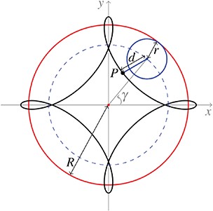
Sketch of a theoretical hypotrochoid curve obtained by tracing a point |$P$| attached to a small circle of radius |$r$| rolling around the inside of a bigger circle of radius |$R$|, where |$d$| is the distance between the point |$P$| and the centre of the small circle. |$\gamma $| is the angle formed by the horizontal axis and the centre of the small rolling circle. The dashed line represents the trace of the centre of the small circle, i.e. a circle of radius |$\widetilde{R}=R-r$|. |$R=2$|, |$r=0.5$| and |$d=0.7$|.
Fixing |$n$|, the value of |$d$| determines if singular points are present, i.e. cusps or self intersections (crunodes). We remark that in Section 3.2.3 we refer to |$n$| as the number of singular points of the curve, however this is a slight abuse of notation since, fixing |$n$|, for some values of |$d$| the curve does not present any singular point and can be described as a rounded approximation of a |$n$|-sided regular polygon. Note that |$d$| admits positive and negatives values; at |$\gamma =0$|, if |$d>0$| the point |$P$| is chosen to the right of the small circle centre, otherwise if |$d<0$| the point |$P$| is chosen to the left. Moreover, the point |$P$| can be chosen to be either inside (|$|d|<r$|), outside (|$|d|>r$|) or on the circumference of the small circle (|$|d|=r$|). The case of |$d=r>0$| corresponds to hypocycloid curves, while the limit case of |$d=0$| corresponds to a circle of radius |$\widetilde{R}$|.
Fitting sperm trajectory data to hypotrochoid curves involves different mathematical challenges. Starting from finding the best minimization algorithm and initial value to approximate the three parameters, |$(\widetilde{R},d,n)$| or |$(R,r,d)$|, that uniquely identify the curve. To our knowledge, there is only one result available in the literature on least-squares hypotrochoid curve fitting in Sinnreich (2016), where a method for a particular case of hypotrochoid curve is presented, i.e. rounded approximation of regular polygons with no cusps and no self intersections. A further challenge comes form the fact that for each data point the corresponding |$\gamma $| is also an unknown, since by definition |$\gamma $| is in general not equal to the point polar angle |$\theta $|. We can relate |$\theta $| and |$\gamma $| using the inverse tangent of the ratio between the |$y$| and |$x$| coordinates of the data point. However, this correspondence is not one-to-one when self intersections are present in the hypotrochoid curve. For this reason, we chose to use the method reported in Woolley (1998) to approximate the simulation f-curves with a hypotrochoid curve. This method exploits the definition of a hypotrochoid curve as two circular motions, and uses geometric and physical principles to estimate the curve parameters without utilizing a minimization algorithm, and can be used for approximating any kind of hypotrochoid curves, including ones that exhibit self intersections.
Given the data points for the f-curves, we follow Woolley (1998) to find the approximating hypotrochoid curve as detailed below.
Starting at time |$t=9s$|, the roll frequency |$\omega _1$| is estimated as the frequency of a full rotation of the rod first point around its centre of mass;
|$n$| is estimated as the ratio between |$2\pi $| and the mean angular separation between two singular points over a full rotation;
The flagellar frequency is |$\omega _2 = \omega _1(n-1)$|;
- Let |$d_{min}$| and |$d_{max}$| be, respectively, the average minimum and maximum distance from the centre of mass over one rotation, then the remaining hypotrochoid parameters can be estimated as follows:(B.3)$$\begin{equation} d = \frac{d_{max} - d_{min}}{2}, \qquad R = \frac{\omega_1 + \omega_2}{\omega_2} \left( d_{min} + d\right), \qquad r=\frac{\omega_1}{\omega_2} \left( d_{min} + d\right). \end{equation}$$
