A discrete dynamics approach to interbank financial contagion

Abstract

The purpose of this paper is to describe in terms of mathematical models and systems theory the dynamics of interbank financial contagion. Such a description gives rise to a model that can be studied with mathematical tools and will provide a new framework for the study of contagion dynamics complementary to research by simulation studied so far. It provides a better understanding of such financial networks and a unifying network for the research of financial contagion. The mathematical description we present is in terms of Boolean dynamical systems and a linear operator. We relate the properties of the dynamical systems to the properties of the operator.

interbank networks, financial contagion, systemic risk, complex systems, Boolean dynamical systems, linear operators

1. Introduction

The problem of financial contagion in an interbank market is a complex one and many academics studied this problem to understand how bank failures affect the financial stability and to shed light into systemic risk. Studying the financial system as a network is one of the methods to investigate the emergence of systemic risks through the interconnections of the banks. In such network structure, every node represents a bank and the capital flows (loans) between banks are represented by the edges of the network.

The flourishing literature of the recent years has addressed several aspects of the problem of financial contagion. As a result, our understanding of this problem has improved considerably. Many papers have contributed to the effort to reveal and explain the innermost mechanisms that cause or foster the financial contagion (for instance, see Acemoglu et al., 2015; Amini et al., 2016; Caccioli et al., 2014; Cifuentes et al., 2005; Cimini et al., 2015; Cont et al., 2010; De Souza et al., 2016; Elliott et al., 2014; Elsinger et al., 2006; Fink et al., 2016; Freixas et al., 2000; Gai & Kapadia, 2010; Georgescu, 2015; Glasserman & Young, 2015; Glasserman & Young, 2016; Greenwood et al., 2015; Ladley, 2013; Memmel & Sachs, 2013; Nier et al., 2007; Tonzer, 2015). However, the introduction of adequate indicators that objectively assess the robustness of the market and its institutions and are related to measurable features of the institutions is always desirable, since it helps the regulatory system to take targeted actions for eliminating the systemic risk.

The topology of the financial network plays a central role in the problem of contagion and, inevitably, has become the topic of many studies (see Acemoglu et al., 2015; Allen & Gale, 2000; Anand et al., 2015; Bardoscia et al., 2017; Iori et al., 2006; Mistrulli, 2011). Interconnectedness between banks has a two-pronged role: on the one hand it stabilizes the system by distributing funds in an effective way among banks; on the other hand can make the system prone to financial contagion through the interbank linkages. This feature of economic networks is depicted in this characteristic property (Acemoglu et al., 2015): when the magnitude of negative shocks is small, then a densely connected network contributes to the stability of the system; however, if this magnitude exceeds a certain threshold, then dense interconnections contribute to the spreading of the contagion. Furthermore, recent studies have revealed the importance of institutions that may not be very large, but they have a lot of connections (‘too-connected-to-fail’ theory). Their failure could trigger a severe series of defaults (see Battiston et al., 2012; Caccioli et al., 2012; Chinazzi et al., 2015).

Undoubtedly, some of the main purposes of the aforementioned studies can be summarized as follows: (1) to facilitate the assessment of an interbank network and of the institutions of which it consists; (2) to detect the weak points of the system and how prone the interbank market is to systemic risk; (3) to help the regulators and supervisors of the system to take suitable proactive measures when it is needed (for instance, see De Souza et al., 2016; Elsinger et al. (2006); Glasserman & Young (2016); Huang et al. (2012)). From this point of view, it is always desirable general results about the causes or the mechanism of the contagion or the topology of the network (although their importance cannot be disputed) to be accompanied by quantitative methods for the assessment of a particular network and for the suitable decision policy.

In the present paper, we adopt this kind of approach towards the study of the problem of financial contagion. Our aim is neither to describe the sources of financial contagion in general nor to analyse the role of the network structure. Our purpose is to develop a theoretical framework and a generic method that, given an arbitrary interbank network, will enable us to study the transmission of the contagion within this particular network and its reaction to systemic shocks for all possible combinations of initial defaulted institutions. Our ultimate goal is through this method to elaborate various metrics for the assessment of the network and the banks of which it consists and for the measurement of the total damage that the contagion creates. These metrics evaluate the robustness of the network and classify its institutions from the more vulnerable to the more stable. As a consequence, using finitely many numbers, the regulators and supervisors of an economic network will be able to assess its stability and detect its weak points.

In order to achieve our goal and produce the aforementioned method, we appeal to tools and techniques from mathematics. More precisely, we utilize tools from systems theory, complex systems and operator theory. The theory of complex systems initiated from research related to engineering and computer science (see Karcanias et al., 1995). Nevertheless, it quickly expanded to several other areas and in particular to issues concerning financial research (for example see Galbiati et al., 2013). In the present work, we elaborate a mathematical theory describing in detail the interbank networks using ideas from complex systems.

The fact that the phenomenon of contagion and the systemic risk are associated with a plethora of multiple and complicated factors cannot be disputed. For instance, except the interbank lending, financial contagion is related to the existence of multiple different financial contracts, multiple types of financial institutions, the presence of uncertainty in the balance sheet size of financial institutions, the constraints of the policies that could be implemented, the characteristics of the market in which the institutions operate, the stock market performance, etc. Furthermore, socio-economic factors can also create or affect the contagion, for example the unemployment rate, the decline in consumption, environmental disasters, etc. Finally, the fact that all these factors are not time invariant cannot be omitted either.

The extended literature of the past 20 years contains investigations that take into account several of the above factors. Nevertheless, the complexity of the problem of contagion and the fact that different factors follow different rules (for example, some could be described with stochastic models, while others with differential equations etc.) makes impossible the evolution of an abstract mathematical theory involving several causes of the financial contagion. For this reason, theoretical studies usually focus on the most significant factors (interconnectedness, interbank lending, capitals) (see Acemoglu et al., 2015; Amini et al., 2016; Barucca et al., 2016; Gai & Kapadia, 2010; Gandy & Veraart, 2016), and computer simulation has emerged as one of the main tools for analysing interbank networks (see Gai & Kapadia, 2010; Greenwood et al., 2015; Hałaj & Kok, 2013; Iori et al., 2006; Leventides et al., 2019; Upper, 2011). Consequently, in this piece of work, we are not aiming at addressing all the issues relevant to financial contagion, but we concentrate on the more important ones, which actually lay in the core of the economic crisis of 2007–2009. Therefore, we develop a theoretical framework for the study of contagion dynamics that also corresponds to a realistic example. Finally, we believe that this framework could be a model for similar studies in the future, which will combine or focus on other parameters of financial contagion.

The rest of the paper is organised as follows. In Section 2, we model the transmission of financial contagion in an interbank network. We define the contagion map, which plays a central role throughout this work, and we study its properties. This map enriches the powerset |$2^X$| of the set |$X$| of banks with a tree structure. Section 3 shows that the contagion map can be described in terms of Boolean dynamical systems. In Section 4, several metrics for the evaluation of banks and networks are introduced. Section 5 provides information for the calculation of these metrics, while Section 6 gives upper and lower bounds for some of them. In Section 7 and 8, linear operators are used and give further insight to the problem of the transmission of financial contagion in an interbank network. All the ideas contained in this work are illustrated with several examples in Section 9 and, finally, Section 10 concludes the paper.

2. Mathematical modelling of interbank networks and financial contagion

2.1 The interbank network and default contagion

Financial systems can be represented as directed weighted graphs, or networks (see for example Acemoglu et al., 2015; Amini et al., 2016; Cont et al., 2010; Leventides et al., 2019). An interbank network is a triple |$(X, E, C)$|⁠, where

the vertex set is |$X=\{1,2,\ldots , n\}$| and its elements represent financial institutions;
|$C=(c_1, c_2, \ldots , c_n)$| denotes the vector of capitals, i.e. |$c_i$| is the capital of the institution |$i$| representing its ability to absorb losses;
|$E=(E_{ij})_{i,j=1}^n$| is the matrix of bilateral exposures. That is, |$E_{ij}$| stands for the exposure of institution |$i$| to institution |$j$| defined as the value of all liabilities of |$j$| to |$i$| at the date of computation. Clearly, |$E$| is an |$n\times n$| matrix whose diagonal line contains only |$0$|⁠, since banks do not lend to themselves.

Hence, this network can be depicted as a directed weighted graph, whose nodes represent institutions and (weighted) links represent exposures. If we sum up the |$i$|-th column of the matrix |$E$|⁠, then we obtain the total interbank liabilities of the bank |$i$|⁠. Hence, the interbank liabilities vector can be introduced:

$$\begin{align*} &L = \left(L_i\right)_{i=1}^n =\left( \sum_{j=1}^n E_{ji}\right)_{i=1}^n.\end{align*}$$

On the other hand, if we take horizontal summation, the we obtain the total interbank assets of each institution. Hence,

$$\begin{align*} &A =\left(A_i\right)_{i=1}^n = \left( \sum_{j=1}^n E_{ij}\right)_{i=1}^n,\end{align*}$$

is the interbank assets vector.

The mechanism of the financial contagion is as follows. An institution (say |$i$|⁠) defaults when it fails to fulfill a legal obligation, for instance some scheduled debt payment, or when it is unable to service a loan. The defaulted institution cannot meet its liabilities and create loan losses to its creditors. These losses are imputed to the capital of the creditors, leading to a loss of |$E_{ji}$| for the creditor |$j$|⁠. In the case where the loss exceeds the capital, i.e. |$E_{ji}>c_j$|⁠, then the bank |$j$| becomes insolvent. Insolvency may not necessarily imply default, since the bank |$j$| may be able to find some liquidity to serve its obligations. However, financial institutions are funded through short term debt, which must be constantly renewed and depends to the solvency and creditworthiness of the institutions. Consequently, insolvent banks are extremely difficult to raise up their levels of liquidity and it is generally accepted that inadequate capital levels entail the instability of the financial network. Hence, in this work, we consider insolvent banks as defaulted. Furthermore, we recognize that other scenarios to default may exist, which entail the phenomenon of contagion. From this point of view, this work serves as a lower bound of the contagion.

Finally, in line with various studies, we adopt the zero recovery assumption for shock transmission, i.e. the creditor banks loss all their interbank assets held against a defaulting bank. This assumption is a realistic one in the short run and it has been used in the literature to analyze worst case scenarios (see Chinazzi et al., 2015; Gai & Kapadia, 2010; Leventides et al., 2019).

Summarizing, the failure of one or more nodes of the graph may lead other institutions to default and the shock propagation continues creating a cascade of defaults.

2.2 The contagion map

$$\begin{align*} &T(A) = A \cup \left\{ j\in X\setminus A \mid \sum_{i\in A} E_{ji} \geqslant c_j \right\}.\end{align*}$$

It should be highlighted that |$T(A)$| describes the first stage of the interbank network after the failure of the banks |$A$|⁠. The defaulted banks |$T(A)$| create loan losses to other banks and a second round of bankruptcies occurs. The new set of defaulted banks is of course |$T(T(A))$| and the transmission of the crisis continues up to the point where an equilibrium set of the map |$T$| occurs, that is a set |$U\subseteq X$| such that |$T(U)=U$|⁠.

Consequently, to every interbank network |$\left (X, E, C \right )$| we correspond a map |$T\colon 2^X\to 2^X$|⁠. This map has the property |$A\subseteq T(A)$| and it is also clear that |$T(\emptyset )=\emptyset $| and |$T(X)=X$|⁠. However, the contagion map has a wide range of behaviours between two extreme cases. The one is |$T_{nc} \colon 2^X \to 2^X$|⁠, such that

$$\begin{align*} & T_{nc}(A) =A, \quad \textrm{for all}\ A\in 2^X,\end{align*}$$

where there is no contagion and the other is |$T_{tc} \colon 2^X \to 2^X$|⁠, such that

$$\begin{align*} &T_{tc}(A) =X, \quad \textrm{for every}\ A\ne \emptyset,\ \textrm{and}\ T_{tc}(\emptyset)=\emptyset,\end{align*}$$

in which case we have total contagion. Our purpose now is to study the contagion map.

2.3 The contagion relation

$$\begin{align*} & A\leqslant^c B\ \textrm{if and only if}\ B=T^m(A)\ \textrm{for some}\ m\in \mathbb{N},\end{align*}$$

where |$T^0(A)=A$| for every |$A\subseteq X$|⁠, |$T^1=T$| and |$T^m=T\circ T \circ \ldots \circ T$|⁠.

2.4 Maximal and minimal elements of |$(2^X,\leqslant ^c)$|

Our first purpose is to take a closer look at the maximal and minimal elements of the partially ordered set |$(2^X,\leqslant ^c)$|⁠. Recall that an element |$A$| of a partially ordered set |$(\mathfrak{H},\leqslant )$| is said to be maximal (respectively, minimal) if for any |$B\in \mathfrak{H}$|⁠, |$A\leqslant B$| (resp., |$B\leqslant A$|⁠) implies that |$A=B$| (e.g. see Anderson, 1985).

As far as the minimal elements are concerned, if |$A$| is minimal, then for any |$B\ne A$| we can conclude that |$T(B)\ne A$| (otherwise, we would have |$B\leqslant ^c A$| and |$B\ne A$|⁠). Conversely, if |$T(B)\ne A$| for any |$B\ne A$|⁠, then |$A$| is minimal. Indeed, if one could find a set |$B\ne A$| such that |$B\leqslant ^c A$|⁠, then |$A=T^k(B)$| for some |$k\geqslant 1$|⁠, and thus, |$A=T(C)$| for |$C=T^{k-1}(B)$|⁠, which is a contradiction.

Therefore, we have proved the next proposition.

Proposition 2.1

The following holds.

An element |$A\in 2^X$| is |$\leqslant ^c$|-maximal if and only if |$T(A)=A$|⁠.
An element |$A\in 2^X$| is |$\leqslant ^c$|-minimal if and only if |$T(B)\ne A$| for any |$B\ne A$|⁠.

Remark 2.1

If the set |$A$| is a singleton, then it is clear that |$A$| is a minimal set. The converse is not always true. That is, there may be minimal sets containing two or more nodes (banks).

Remark 2.2

A set |$A\in 2^X$| may be simultaneously maximal and minimal. The standard example is the empty set; however, there may be other sets with this property. For instance, if |$A=\{i\}$| is maximal (and, of course, minimal), then this means that the bank |$i$| does not have serious impact on the interbank system, since its default leads no other bank to failure.

Example 2.1

Let us examine the extreme case of the contagion maps |$T_{nc}$| and |$T_{tc}$| mentioned above. In the case of |$T_{nc}$|⁠, we have that any set |$A\in 2^X$| is maximal and minimal at the same time. In the case of total contagion, that is the case of the map |$T_{tc}$|⁠, we have that the only maximal elements are the empty set and the set |$X$| itself. Moreover, in this case, every |$A\ne X$| is a minimal element.

2.5 Chains and circles of |$(2^X, \leqslant ^c)$|

In agreement with standard tools from mathematics (see Anderson, 1985), a subset |$\mathcal{C}$| of the partially ordered set |$(2^X, \leqslant ^c)$| is said to be a chain if for every |$A,B\in \mathcal{C}$| we have |$A\leqslant ^c B$| or |$B\leqslant ^c A$|⁠. A chain |$\mathcal{C}$| is called maximal if there is no chain |$\mathcal{C}^{\prime}$| such that |$\mathcal{C}$| is a proper subset of |$\mathcal{C}^{\prime}$|⁠. Clearly, a maximal chain has the form:

$$\begin{align*} &\mathcal{C} = \left\{{A_1} {\leqslant^c} {A_2} {\leqslant^c} \ldots{\leqslant^c} {A_k} \right\},\end{align*}$$

where |$T(A_j)=A_{j+1}$| for any |$j=1,2, \ldots , k-1$|⁠, |$T(A_k)=A_k$| and |$T(B)\ne A_1$| for any |$B\ne A_1$|⁠. That is, the final term |$A_k$| is an equilibrium set and the first term |$A_1$| is a minimal set.

If |$A$| is any subset of |$X$|⁠, then the following chain can be defined:

$$\begin{align*} &\mathcal{C}_A = \{A, T(A), T^2(A), \ldots, T^m(A) \},\end{align*}$$

where |$m\geqslant 0$| is the least integer such that |$T^m(A)=T^{m+1}(A)$|⁠. (It is clear that such an integer |$m$| exists: the sequence |$A, T(A), T^2(A), \ldots $| cannot consist of infinitely many terms, since |$2^X$| contains only finitely many elements.) In particular, when |$A=\{i\}$| is a singleton, then the chain |$\mathcal{C}_A$| will be denoted by |$\mathcal{C}_i$| and it is a maximal chain.

When the banks belonging to the set |$A$| default, the chain |$\mathcal{C}_A$| describes the development of the crisis through the network. Two features of the chain |$\mathcal{C}_A$| are very important and should be taken into account. The first one is the difference |$\sharp T^m(A) - \sharp A$|⁠, which shows the total number of banks that are affected after the failure of the banks belonging to the set |$A$|⁠. The second one, which should be considered in connection to the first one, is the length of the chain, that is the number |$m$|⁠. This number is related to the time that intervenes between the initial shock and the point where the interbank system is stabilized.

Finally, it is worth mentioning that no chain |$\mathcal{C}= \{A_1\leqslant ^c A_2 \leqslant ^c \ldots \leqslant ^c A_m \}$| can be a circle, that is we cannot have |$A_1 =A_m$|⁠. There is only one exception, namely when |$A\in 2^X$| is both maximal and minimal. Then the corresponding chain is |$\mathcal{C}_A=\{A\}$| and it is trivially a circle.

Example 2.2

In the case of the contagion map |$T_{nc}$|⁠, every |$A\subseteq X$| is maximal and minimal. Consequently, every |$A$| produces a maximal chain |$\{A\}$| consisting of only one element.

In the other extreme case, that is the case of the map |$T_{tc}$|⁠, we have the trivial maximal chain |$\{\emptyset \}$| containing only the empty set, and any |$A\ne X$| gives the maximal chain |$\{A\leqslant ^c X\}$| containing two elements |$A$| and |$X$|⁠.

2.6 Connected components and the tree-structure of |$(2^X, \leqslant ^c)$|

For any maximal element |$A\in 2^X$|⁠, we consider the following collection of subsets of |$X$|⁠:

$$\begin{align*} & P_A= \big\{ B\in 2^X \mid B\leqslant^c A \big\}.\end{align*}$$

In the language of mathematics, a subset |$P$| of a partially ordered set |$(\mathfrak{H},\leqslant )$| is called an upper set if for any |$x\in P$| and any |$x\leqslant y$| we have that |$y$| belongs to |$P$|⁠. Using this terminology, we have that |$P_A$| is an upper set in |$(2^X, \leqslant ^c)$| and we say that |$P_A$| is the upper set corresponding to |$A$|⁠.

The upper sets |$\{P_A \mid A \textrm{maximal}\}$| define a partition of |$2^X$| in the following sense.

Proposition 2.2

For the upper sets the following hold:

(i) Any set |$B\subseteq X$| belongs to the upper set |$P_A$| for some maximal set |$A\in 2^X$|⁠, that is
$$\begin{align*} &\bigcup_{A: \textrm{maximal}} P_A = X.\end{align*}$$
(ii) If |$A\ne A^\prime $| are maximal, then |$P_A$| and |$P_{A^\prime }$| are disjoint sets.

The proof is standard, however, it will be given for sake of completeness.

Proof.

For any set |$B\subseteq X$| the chain |$\mathcal{C}_B = \{B, T(B), \ldots , T^m(B) \}$| has been defined, where |$A=T^m(B)$| is a maximal element. Clearly, |$B\leqslant ^c A$| and |$B$| belongs to |$P_A$|⁠.

Suppose now that |$B\in P_A \cap P_{A^\prime }$|⁠, where |$A,A^\prime $| are maximal. Then |$A=T^k(B)$| and |$A^\prime =T^m(B)$| for some integers |$k,m\geqslant 0$|⁠. If |$k=m$|⁠, we have |$A=A^\prime $|⁠. Without loss of generality we assume that |$k<m$|⁠. Then:

$$\begin{align*} &A^\prime =T^m(B) = T^{m-k} \circ T^k(B) =T^{m-k}(A) =A,\end{align*}$$

where the last equation follows from the fact that |$A$| is maximal. Therefore, if |$A\ne A^\prime $|⁠, then the upper sets |$P_A, P_{A^\prime }$| are disjoint.

Because of the above proposition, we will also say that |$\{ P_A \mid A \textrm{maximal}\}$| are the connected components of the contagion graph |$(2^X, \leqslant ^c)$|⁠.

Each component |$P_A$|⁠, A being maximal, has a tree structure. The maximal set |$A$| is located at the highest level of the tree. At the lowest levels there are some minimal sets |$(B_i)_{i\in I}$|⁠. Then, |$P_A$| consists of the maximal chains |$\mathcal{C}_{B_i}$|⁠, |$i\in I$|⁠, starting from |$B_i$| and ending at |$A$|⁠.

Example 2.3

In the case of the contagion map |$T_{nc}$|⁠, every set |$A\subseteq X$| is maximal and forms itself a connected component |$P_A=\{A\}$|⁠.

In the case of |$T_{tc}$|⁠, we have only two maximal sets |$\emptyset , X$|⁠. Therefore, |$2^X$| is composed of two connected components: |$P_\emptyset =\{\emptyset \}$| and |$P_X=\{A\subseteq X \mid A\ne \emptyset \}$|⁠.

3. Boolean dynamical systems

In the previous section, we defined the contagion map |$T\colon 2^X \to 2^X$| and we studied the structure of the generated partially ordered set |$(2^X, \leqslant ^c)$|⁠. However, handling the powerset |$2^X$| of a set |$X$| is not always easy and mainly it is not suitable for calculation purposes. In the present section, we provide an equivalent description of the contagion map using Boolean dynamical systems.

It is a standard approach to identify the powerset |$2^X$| of the set |$X=\{1,2,\ldots , n\}$| with |$\mathbb{Z}_2^n =\{0,1\}^n$|⁠, i.e. the set of vectors of length |$n$| whose entries are |$0$| or |$1$|⁠. Indeed, any subset |$A$| of |$X$| can be identified with the indicator vector |$\textbf{1}_{\textbf{A}} \in \mathbb{Z}_2^n$| of |$A$|⁠, which has zero entries everywhere except the coordinates corresponding to the numbers belonging to |$A$|⁠. (In our setting, |$1$| means that the corresponding node defaults, and |$0$| means that the node does not default.) The map

$$\begin{align*} & 2^X \to \mathbb{Z}_2^n\end{align*}$$

$$\begin{align*} &A \mapsto \boldsymbol{1_A},\end{align*}$$

defines a one-to-one and onto correspondence between |$2^X$| and |$\mathbb{Z}_2^n$|⁠. Throughout this paper, following the standard approach, we sometimes will make no distinction between |$A$| and |$\textbf{1}_{\textbf{A}}$| or between |$2^X$| and |$\mathbb{Z}_2^n$|⁠. Furthermore, the vector |$\textbf{1}_{\textbf{X}}=(1,1,\ldots 1)$| will also be denoted by |$\textbf{1}$|⁠.

As a consequence of the above observations, the contagion map |$T\colon 2^X \to 2^X$| can be identified with the map |$ \mathbb{Z}_2^n \to \mathbb{Z}_2^n$|⁠, where, |$\textbf{1}_{\textbf{A}}\mapsto \boldsymbol{1_{T(A)}}$|⁠. With a slight abuse of notation, we will also denote the aforementioned map by |$T$|⁠. Therefore, the contagion map |$T$| can be seen as

$$\begin{align*} & T\colon \mathbb{Z}_2^n \to \mathbb{Z}_2^n\end{align*}$$

$$\begin{align*} &\boldsymbol{1_A}\mapsto T(\boldsymbol{1_A}) \equiv \boldsymbol{1_{T(A)}}.\end{align*}$$

Calculating the value of |$T(\textbf{1}_{\textbf{A}})$| requires two more ingredients. The first one is a slight modification |$E_0$| of the exposures matrix |$E$|⁠. The matrix |$E_0$| follows from |$E$| by replacing the zero diagonal of the latter with the vector |$C$| of capitals. In other words

$$\begin{align*} &E_0 = \left[ \begin{array}{cccc} c_1 & E_{12} & \ldots & E_{1n} \\ E_{21} & c_2 & \ldots & E_{2n} \\ \vdots & \vdots & \vdots & \vdots \\ E_{n1} & E_{n2} & \ldots & c_n \end{array} \right] .\end{align*}$$

The second ingredient is the function

$$\begin{align*} &f\colon \mathbb{R}^n \to \mathbb{Z}_2^n\end{align*}$$

defined by

$$\begin{align*} &f(\textbf{x})(i) = \left\{ \begin{array}{ll} 1, & \textbf{x}(i)\leqslant\ \hbox{0}; \\ 0, & \textbf{x}(i)>\ \hbox{0}. \end{array} \right. \end{align*}$$

where |$\textbf{x}$| denotes a vector and |$\textbf{x}(i)$| stands for the |$i$|-th coordinate of this vector. Then, we have the following proposition.

Proposition 3.1

The contagion map |$T$| is given by the following Boolean dynamical system:

$$\begin{align*} &T(\boldsymbol{1_A}) = f(C - E_0 \cdot \boldsymbol{1_A})\ \textrm{for any subset}\ A\ \textrm{of}\ X.\end{align*}$$

Proof.

We have to prove that

$$\begin{align*} &\boldsymbol{1_{T(A)}}= f(C - E_0 \cdot \boldsymbol{1_A}).\end{align*}$$

This is equivalent to the statement: for any |$j=1,2,\ldots , n$|⁠,

$$\begin{align*} j\in T(A)\ \text{if and only if the }\textit{j}\text{-th coordinate of}\ f(C - E_0 \cdot \textbf{1}_{\textbf{A}})\ \textrm{is equal to}\ 1. \end{align*}$$

Or equivalently, for any |$j=1,2,\ldots , n$|⁠,

$$\begin{align*} j\in T(A)\ \text{if and only if the }\textit{j}\text{-th coordinate of}\ C - E_0 \cdot \textbf{1}_{\textbf{A}}\ \text{is non-positive}.\end{align*}$$

We now distinguish two cases.

Case I: If |$j\in A$| (which implies that |$j\in T(A)$|⁠), then the |$j$|-th coordinate of the vector |$E_0 \cdot \textbf{1}_{\textbf{A}}$| is equal to |$c_j+\sum _{i\in A, i\ne j} E_{ji}$|⁠. Hence, the |$j$|-th coordinate of |$C - E_0 \cdot \textbf{1}_{\textbf{A}}$| is |$-\sum _{i\in A, i\ne j} E_{ji}$|⁠, and it is non-positive.

Case II: If |$j \notin A$|⁠, then the |$j$|-th coordinate of the vector |$C-E_0 \cdot \textbf{1}_{\textbf{A}}$| is equal to |$c_j-\sum _{i\in A} E_{ji}$|⁠. By the definition of the contagion map, we observe that

$$\begin{align*} j\in T(A) & \Leftrightarrow \sum_{i\in A} E_{ji} \geqslant c_j \\ & \Leftrightarrow \textrm{the}\ j\text{-th coordinate of}\ C - E_0 \cdot \boldsymbol{1_A}\ \text{is non-positive}. \end{align*}$$

The desired result holds in both cases and the proof is complete.

4. Quantitative analysis of the contagion

The purpose of the present section is to introduce several parameters that quantify and measure the contagion of a financial shock through the interbank network. Hence they facilitate the assessment of the network and of the banks of which it consists and they help to the better understanding of the mechanism and the consequences of the contagion.

4.1 The contagion vector

We start with the contagion vector that constitutes the backbone of the assessment of the banks belonging to the network. It is defined as follows:

$$\begin{align}& V= \sum_{A\in 2^X} \left(\boldsymbol{1_{T(A)}} - \boldsymbol{1_A} \right) \in \mathbb{Z}^n. \end{align}$$

(4.1)

Example 4.1

In the case of the contagion map |$T_{nc}$|⁠, since |$T_{nc}(A)=A$| for any subset |$A\in 2^X$|⁠, it follows that the contagion vector is clearly the zero vector. However, the other extreme case, that is that of the map |$T_{tc}$| is of more importance. As we will make use of it in the sequel, we isolate it here and it is given in the next proposition.

Proposition 4.1

For the contagion map |$T_{tc}(A)=X$| for all non-empty |$A\in 2^X$|⁠, the corresponding contagion vector is

$$\begin{align*} &V_{tc}= (2^{n-1}-1) \textbf{1}.\end{align*}$$

Proof.

We have

$$\begin{align*} &V_{tc} = \sum_{A\in 2^X} (\boldsymbol{1_{T_{tc}(A)}}-\boldsymbol{1_A}) = \sum_{A\in 2^X, A\ne \emptyset} (\boldsymbol{1_X}-\boldsymbol{1_A}) = \sum_{A\in 2^X, A\ne \emptyset} \boldsymbol{1_{X\setminus A}} = \sum_{A\in 2^X, A\ne X} \boldsymbol{1_A}.\end{align*}$$

Consequently, the |$i$|-th coordinate of the vector |$V_{tc}$| is equal to the number of all subsets |$A$| of |$X$| with the property that |$A\ne X$| and |$i\in A$|⁠. It follows that the coordinates of |$V_{tc}$| are independent from |$i$| and, hence, they are equal to each other. Furthermore, we observe the following: there is only one subset |$A$| of cardinality |$1$| containing |$i$|⁠; there are |$ {n-1}\choose{1}$| subsets of cardinality |$2$| that contain the element |$i$|⁠; continuing in a similar way, we finally have |$ {n-1}\choose{n-2}$| subsets of |$X$| of cardinality |$n-1$| containing |$i$|⁠. Therefore, each and every coordinate of |$V_{tc}$| is equal to

$$\begin{align*} &\binom{n-1}{0} + \binom{n-1}{1} +\ldots +\binom{n-1}{n-2} = \sum_{k=0}^{n-1} \binom{n-1}{k} - \binom{n-1}{n-1}= 2^{n-1}-1.\end{align*}$$

Consequently, |$V_{tc} = (2^{n-1}-1) \textbf{1}$| and the proof is complete.

4.2 Indicators

We next introduce some indicators that enable the measurement of the total damage to which the interbank network is subject and, hence, the assessment of the whole network. It should be pointed out that in this context the term ‘total damage’ does not refer to the total losses of the system at the end of the contagion process, but rather refers to the losses that the system might experience given all possible choices of initially defaulted entities.

Assume that |$A$| is a subset of the set of all banks, that is |$A\in 2^X$|⁠.

(i) Firstly, we set |$\textrm{ind}_1 (A) = \sharp A$|⁠. Therefore, in the case of financial shock, the indicator |$\textrm{ind}_1 (A)$| measures the banks that failures. Clearly, this indicator is given by the inner product: |$\textrm{ind}_1 (A) = \left \langle \textbf{1}_{\textbf{A}}, \textbf{1} \right \rangle $|⁠, where |$\textbf{1}$| is the vector whose all entries are equal to |$1$|⁠.
(ii) Secondly, we let |$\textrm{ind}_2 (A)$| be the sum of the capitals possessed by the banks of the set |$A$|⁠. These capitals are withdrawn from the market after the collapse of the banks of the set |$A$|⁠. It is easy to see that |$\textrm{ind}_2 (A) =\left \langle \textbf{1}_{\textbf{A}}, C \right \rangle $|⁠, for any |$A\subseteq X$|⁠.
(iii) |$\textrm{ind}_3 (A)$| is the sum of the liabilities of the banks of the set |$A$|⁠. In other words, |$\textrm{ind}_3 (A)$| is the sum of the weights of those edges of the interbank graph whose end is some node corresponding to a bank of the set |$A$|⁠. Using the liabilities vector |$L$|⁠, we have the following formula: |$ \textrm{ind}_3 (A) = \left \langle \textbf{1}_{\textbf{A}}, L \right \rangle $|⁠.

Returning to the contagion map |$T\colon \mathbb{Z}_2^n \to \mathbb{Z}_2^n$|⁠, each one of the above-mentioned indicators produce the total indicator of the contagion which for any |$i=1,2,3$| is defined as follows:

$$\begin{align*} &m_i(T) = \frac{\sum_{A\in 2^X} \left(\textrm{ind}_i (T(A)) - \textrm{ind}_i (A)\right)}{M_i},\end{align*}$$

where,

$$\begin{align*} M_i &= \sum_{A\in 2^X} \left(\textrm{ind}_i (X) - \textrm{ind}_i (A)\right)\\ & = 2^{\sharp X} \cdot \textrm{ind}_i (X) -\sum_{A\in 2^X} \textrm{ind}_i (A). \end{align*}$$

That is, |$M_i$| is the maximum value of the numerator, which is taken in the case of total contagion, i.e. the case of the map |$T_{tc}$|⁠. Consequently, the quantities |$m_1(T), m_2(T), m_3(T)$| take values between |$0$| and |$1$| and measure the level of contagion in the network. The first indicator estimates the proportion of the banks that are affected, |$m_2(T)$| and |$m_3(T)$| are related to the capitals that are destroyed and to the loans that are not paid back respectively.

The above-mentioned indicators are related to the contagion vector. For the first indicator this connection is given in the next proposition.

Proposition 4.2

For the contagion map |$T\colon \mathbb{Z}_2^n \to \mathbb{Z}_2^n$|⁠, with corresponding contagion vector |$V$|⁠, the indicator |$m_1(T)$| is given by

$$\begin{align*} & m_1(T) = \frac{\left\langle V,\textbf{1} \right\rangle}{n\cdot (2^{n-1}-1)}.\end{align*}$$

Proof.

By the fact that |$\textrm{ind}_1 (A) = \left \langle \textbf{1}_{\textbf{A}}, \textbf{1} \right \rangle $|⁠, for any |$A\in 2^X$|⁠, and by the linearity of the inner product, it follows that

$$\begin{align*} \sum_{A\in 2^X}\left(\textrm{ind}_1 (T(A))-\textrm{ind}_1 (A)\right)&=\sum_{A\in 2^X} \left(\left\langle \boldsymbol{1_{T(A)}},\textbf{1} \right\rangle-\left\langle \boldsymbol{1_A}, \textbf{1} \right\rangle\right) \\ &= \sum_{A\in 2^X} \left\langle \boldsymbol{1_{T(A)}}-\boldsymbol{1_A},\textbf{1} \right\rangle \\ &= \left\langle \sum_{A\in 2^X}\left(\boldsymbol{1_{T(A)}}-\boldsymbol{1_A}\right),\textbf{1} \right\rangle \\ &= \left\langle V, \textbf{1} \right\rangle. \end{align*}$$

With the same reasoning, we have that

$$\begin{align*} & M_1= \sum_{A\in 2^X}\left(\textrm{ind}_1 (T_{tc}(A))-\textrm{ind}_1 (A)\right) = \left\langle V_{tc}, \textbf{1} \right\rangle. \end{align*}$$

By Proposition 4.1, we know that |$V_{tc}= (2^{n-1}-1) \textbf{1}$|⁠. Hence,

$$\begin{align*} & M_1= \left\langle (2^{n-1}-1) \textbf{1}, \textbf{1} \right\rangle= n\cdot (2^{n-1}-1). \end{align*}$$

Finally, it follows that

$$\begin{align*} &m_1(T) = \frac{\left\langle V, \textbf{1} \right\rangle}{\left\langle V_{tc}, \textbf{1} \right\rangle} = \frac{\left\langle V, \textbf{1} \right\rangle}{ n\cdot (2^{n-1}-1)}.\end{align*}$$

Since the indicators |$\textrm{ind}_2 (A)$| and |$\textrm{ind}_3 (A)$| are also written in the form of some inner product, the same argumentation as in the proof of Proposition 4.2, replacing |$\textbf{1}$| with |$C$| and |$L$|⁠, respectively, proves the next formulas for |$m_2(T)$| and |$m_3(T)$|⁠.

Proposition 4.3

For any contagion map |$T\colon 2^X \to 2^X$| the following holds:

$$\begin{align*} &m_2(T) = \frac{\left\langle V, C \right\rangle}{(2^{n-1}-1)\left\langle \textbf{1},C \right\rangle}\end{align*}$$

$$\begin{align*} &m_3(T) = \frac{\left\langle V, L \right\rangle}{(2^{n-1}-1)\left\langle \textbf{1},L \right\rangle}.\end{align*}$$

Example 4.2

When there is no contagion, that is we have the map |$T_{nc} (A)=A$| for every |$A\in 2^X$|⁠, then we have seen that the contagion vector |$V_{nc}$| is the zero vector. By the previous propositions, it follows that:

$$\begin{align*} &m_1(T_{nc}) = m_2(T_{nc}) =m_3(T_{nc})=0.\end{align*}$$

In the other extreme case, that is the case of total contagion |$T_{tc}(A)=A$| for every |$A\ne \emptyset $|⁠, we have that |$V_{tc}=(2^{n-1}-1) \textbf{1}$|⁠. Hence, the previous propositions imply that

$$\begin{align*} &m_1(T_{tc}) = m_2(T_{tc}) =m_3(T_{tc})=1.\end{align*}$$

5. Calculation of the contagion vector and the indicators

In this section, we examine how the tree-structure of the powerset |$2^X$| affects the calculation of the contagion vector and, therefore, of the indicators. More specifically, it is proved that the contagion vector depends only on the maximal, the minimal and the cross elements of |$2^X$| (defined below).

From Section 2, we already know that the powerset |$2^X$| can be decomposed into its connected components:

$$\begin{align*} &\big\{ P_A \mid A \ \textrm{maximal element of}\ 2^X \big\}.\end{align*}$$

Since these components are pairwise disjoint, we have that

$$\begin{align*} &V = \sum_{A\ \textrm{maximal}} V_A,\end{align*}$$

where,

$$\begin{align*} &V_A = \sum_{D\in P_A} \left(\boldsymbol{1_{T(D)}} - \boldsymbol{1_D} \right).\end{align*}$$

Therefore, it suffices to estimate the vector |$V_A$|⁠. Towards this direction, we recall, again from Section 2, that each component |$P_A$| has a tree structure. At the highest level of the tree we find the maximal set |$A$| and at the lowest levels of the tree there are some minimal sets |$B_{i_1}, B_{i_2}, \ldots , B_{i_k}$|⁠. The component |$P_A$| is composed of the maximal chains |$\mathcal{C}_t$| starting from |$B_{i_t}$| and ending at |$A$|⁠. Changing the enumeration if necessary, we may assume that

$$\begin{align*} &l(\mathcal{C}_1) \geqslant l(\mathcal{C}_2) \geqslant \ldots l(\mathcal{C}_k),\end{align*}$$

where |$l(\mathcal{C}_t)$| denotes the length of the chain |$\mathcal{C}_t$|⁠.

Now, we set |$A_1=A$| and for each chain |$\mathcal{C}_t$| we denote by |$A_t$| the biggest (with respect to the partial order |$\leqslant ^c$|⁠) element of |$\mathcal{C}_t$| belonging to |$\cup _{j=1}^{t-1} \mathcal{C}_j$|⁠. Geometrically it is easy to detect the sets |$A_t$|⁠, since (with the exception of |$A_1$|⁠) they are those sets of |$P_A$| in which at least two chains cross each other. For this reason, the |$A_t$|’s are said to be the cross elements of |$2^X$|⁠.

Let |$\widetilde{\mathcal{C}}_t$| be the following subchain of |$\mathcal{C}_t$|⁠:

$$\begin{align*} &\widetilde{\mathcal{C}}_t = \left\{ D\in \mathcal{C}_t \mid{B_{i_t}} {\leqslant^c} {D <^c} {A_t} \right\}.\end{align*}$$

Then,

$$\begin{align*} &V_A= \sum_{D\in P_A} \left(\boldsymbol{1_{T(D)}} - \boldsymbol{1_D} \right) = \sum_{t=1}^k \sum_{D\in \widetilde{\mathcal{C}}_t} \left(\boldsymbol{1_{T(D)}} - \boldsymbol{1_D}\right).\end{align*}$$

However, if |$\widetilde{\mathcal{C}}_t= \{ D_1\leqslant ^c D_2 \leqslant ^c \ldots \leqslant ^c D_q \}$|⁠, with |$ D_1= B_{i_t}$| and |$T(D_q)=A_t$|⁠, then we have |$T(D_j) = D_{j+1}$|⁠, and therefore

$$\begin{align*} \sum_{D\in \widetilde{\mathcal{C}}_t} \left(\boldsymbol{1_{T(D)}} -\boldsymbol{1_D}\right) &= \sum_{j=1}^q \left(\boldsymbol{1_{T(D_j)}} - \boldsymbol{1_{D_j}}\right)\\ &= \sum_{j=1}^q \left(\boldsymbol{1_{D_{j+1}}} - \boldsymbol{1_{D_j}}\right)\\ &= \boldsymbol{1_{D_{q+1}}} - \boldsymbol{1_{D_1}} \\ &= \boldsymbol{1_{A_t}} - \boldsymbol{1_{B_{i_t}}} \end{align*}$$

Hence, it follows that

$$\begin{align*} &V_A=\sum_{D\in P_A} \left(\boldsymbol{1_{T(D)}} - \boldsymbol{1_D}\right) = \sum_{t=1}^k \left(\boldsymbol{1_{A_t}} - \boldsymbol{1_{B_{i_t}}} \right).\end{align*}$$

Consequently, in order to calculate the contagion vector, it suffices to know the maximal, minimal and cross elements of |$2^X$|⁠. By Propositions 4.2 and 4.3, this is also true for the indicators |$m_1(T)$|⁠, |$m_2(T)$| and |$m_3(T)$|⁠.

6. Upper and lower bounds

Our next concern is to provide upper and lower bounds for the first indicator |$m_1(T)$| of the contagion map of an interbank system, under the hypothesis that the number of equilibrium sets of |$T$| is known. Since |$m_1(T)$| is given by

$$\begin{align*} &m_1(T) = \frac{\sum_{A\in 2^X} \left(\textrm{ind}_1 (T(A)) - \textrm{ind}_1 (A)\right)}{n\cdot (2^{n-1}-1)},\end{align*}$$

it suffices to find bounds for the quantity in the numerator.

6.1 Lower bound

We observe that for any fixed point |$A\in 2^X$|⁠, i.e. for any maximal element |$A$| of |$(2^X, \leqslant ^c)$|⁠, we have |$T(A)=A$| and, therefore, |$\textrm{ind}_1 (T(A)) - \textrm{ind}_1 (A)=0$|⁠. If |$A$| is not a fixed point, then |$T(A)$| contains at least one more bank than the set |$A$|⁠. Consequently, |$\textrm{ind}_1 (T(A)) - \textrm{ind}_1 (A)\geqslant 1$|⁠. Hence, if the number of fixed points is equal to |$f$| (⁠|$2\leqslant f\leqslant 2^n$|⁠), we obtain

$$\begin{align*} \sum_{A\in 2^X} \left(\textrm{ind}_1 (T(A)) - \textrm{ind}_1 (A)\right) &= \sum_{A\ \textrm{not fixed point}} \left(\textrm{ind}_1 (T(A)) - \textrm{ind}_1 (A)\right)\\ &\geqslant \sum_{A\ \textrm{not fixed point}} 1 = 2^n-f. \end{align*}$$

Thus, the following proposition has been proved.

Proposition 6.1

Let |$T$| be the contagion map of an interbank network system consisting of |$n$| banks. If the number of fixed points of |$T$| is equal to |$f$|⁠, |$2\leqslant f\leqslant 2^n$|⁠, then the next inequality holds:

$$\begin{align*} &m_1(T) \geqslant \frac{2^n-f}{n\cdot (2^{n-1}-1)}.\end{align*}$$

6.2 Upper bound

For any |$k=0,1,2,\ldots ,n$|⁠, we denote by |$d_k$| the number of the subsets of |$X$| that contain at most |$k$| elements. Since there are |$\binom{n}{j}$| sets |$A\in 2^X$| containing exactly |$j$| elements, it follows that

$$\begin{align*} &d_k = \sum_{j=0}^k \binom{n}{j}, \quad \textrm{for any}\ k=0,1,\ldots, n.\end{align*}$$

Clearly, |$d_0 = { {n}\choose{0}}=1$| and |$d_n= \sum _{j=0}^n {{n}\choose{j}} =2^n$|⁠.

Theorem 6.1

Let |$T\colon \mathbb{Z}_2^n \to \mathbb{Z}_2^n$| be the contagion map of an interbank network system consisting of |$n$| banks. Assume that the number of fixed points of |$T$| is equal to |$f$|⁠, |$2\leqslant f\leqslant 2^n$|⁠. Let also |$k\in \{0,1,\ldots ,n\}$| be such that |$d_k\leqslant 2^n-f < d_{k+1}$|⁠. Then the next inequality holds:

$$\begin{align*} &\sum_{A\in 2^X} \left(\textrm{ind}_1 (T(A)) - \textrm{ind}_1 (A)\right) \leqslant \sum_{i=1}^k \binom{n}{i} \cdot (n-i) + (2^n -f -d_k+1)\cdot (n-k-1). \end{align*}$$

Proof.

We have |$\textrm{ind}_1 (T(A)) - \textrm{ind}_1 (A)=0$| for any maximal element |$A$| of |$(2^X,\leqslant ^c)$|⁠. Moreover, |$\textrm{ind}_1 (T(A))\leqslant n$| for any set |$A\in 2^X$|⁠. Therefore, we obtain

$$\begin{align*} \sum_{A\in 2^X} \left(\textrm{ind}_1 (T(A)) - \textrm{ind}_1 (A)\right) & = \sum_{A\ \textrm{not maximal}} \left(\textrm{ind}_1 (T(A)) - \textrm{ind}_1 (A)\right) \\ & \leqslant \sum_{A\ \textrm{not maximal}} \left(n - \textrm{ind}_1 (A)\right). \end{align*}$$

If one wishes to maximize the last sum, then they have to choose the |$2^n-f$| not maximal sets |$A$| so that their cardinality to be as small as possible. Since the empty set is maximal, we can choose the |$ {n}\choose{1}$| sets of cardinality |$1$|⁠, the |$ {n}\choose{2}$| sets of cardinality |$2$| and so on. This procedure ends when we choose the |$ {n}\choose{k}$| sets of cardinality |$k$|⁠. The remaining sets, whose number is

$$\begin{align*} &2^n-f-\left(\binom{n}{1} +\binom{n}{2}+\ldots+\binom{n}{k}\right) =2^n-f-\left(d_k-1\right) =2^n-f-d_k+1,\end{align*}$$

will be chosen arbitrarily from the family of subsets of |$X$| whose cardinality is equal to |$k+1$|⁠. Consequently,

$$\begin{align*} &\sum_{A\in 2^X} \left(\textrm{ind}_1 (T(A)) - \textrm{ind}_1 (A)\right) \leqslant \sum_{i=1}^{k} \binom{n}{i} \cdot (n-i) + (2^n-f-d_k+1) (n-k-1),\end{align*}$$

and we have obtained the desired result.

Corollary 6.1

Under the hypotheses of Theorem 6.1, it follows that

$$\begin{align*} &m_1(T) \leqslant \frac{\sum_{i=1}^k \binom{n}{i} \cdot (n-i) + (2^n -f -d_k+1)\cdot (n-k-1)}{n\cdot (2^{n-1}-1)}.\end{align*}$$

7. Description through linear operators

In order to delve deeper into the study of financial contagion problem and to enrich the interbank system with more structural properties, we appeal to linear operators between vector spaces. We denote by |$(e_i)_{i=1}^{2^n}$| the usual vector basis of |$\mathbb{R}^{2^n}$|⁠, that is |$e_i$| is zero everywhere except the |$i$|-th coordinate that equals |$1$|⁠. Furthermore, we consider a one-to-one correspondence |$\varPhi \colon \mathbb{Z}_2^n \to \mathbb{R}^{2^n}$| from |$\mathbb{Z}_2^n$| onto the basis |$(e_i)_{i=1}^{2^n}$|⁠, with the following property:

$$\begin{align*} \textbf{(P)}\!: \textrm{if}\ \textbf{x},\textbf{y}\in \mathbb{Z}_2^n\ \textrm{with}\ \varPhi (\textbf{x})&=e_i, \varPhi (\textbf{y})=e_j\ \text{and the number of 1's appearing in}\ \textbf{x}\ \textrm{is less than or equal}\\ &\quad\ \text{to the number of 1's appearing in }\textbf{y},\ \textrm{then}\ i<j. \end{align*}$$

It is easy to find a map |$\varPhi $| with the desired property. For instance, let us fix the following map:

$$\begin{align*} &\varPhi (0,0,\ldots,0) = e_1, \quad \varPhi (1,0,\ldots,0) = e_2, \quad \varPhi (0,1,\ldots, 0) = e_3, \quad \ldots \quad \varPhi (0,0,\ldots,1) = e_{n+1},\end{align*}$$

then we continue with the elements of |$\mathbb{Z}_2^n$| which have two entries equal to |$1$|⁠:

$$\begin{align*} &\varPhi (1,1,0, \ldots,0) = e_{n+2}, \quad \varPhi (1,0,1,\ldots,0) = e_{n+3}, \quad \ldots \quad \varPhi (1,0,\ldots, 1) = e_{2n+1} \ldots\end{align*}$$

and so on.

The contagion map |$T\colon \mathbb{Z}_2^n \to \mathbb{Z}_2^n$| gives rise to a map |$S_T\colon (e_i)_{i=1}^{2^n} \to (e_i)_{i=1}^{2^n}$| via the formula |$S_T(e_i) = \varPhi T \varPhi ^{-1}(e_i)$|⁠. The map |$S_T$| can be extended linearly to the vector space |$\mathbb{R}^{2^n}$| and a linear operator is produced, which is also denoted by |$S_T\colon \mathbb{R}^{2^n} \to \mathbb{R}^{2^n}$|⁠. The operator |$S_T$| is represented by a |$2^n \times 2^n$|-matrix |$M_T$|⁠. When the vector |$S_T(e_i)$| is written as a linear combination of the vectors of the basis |$(e_j)_{j=1}^{2^n}$| then the coefficients form the |$i$|-th column of the matrix |$M_T$|⁠. Since |$S_T(e_i)$| is itself an element of the basis |$(e_j)_{j=1}^{2^n}$|⁠, it follows that the entries of |$M_T$| are |$0$| or |$1$| and that there is exactly one |$1$| in each column of |$M_T$|⁠.

Proposition 7.1

The eigenvalues of |$S_T$| (and of |$M_T$|⁠) are independent from the correspondence |$\varPhi $|⁠.

Proof.

Assume that |$\varPsi \colon \mathbb{Z}_2^n \to (e_i)_{i=1}^{2^n}$| is a one-to-one and onto map satisfying property (P). Let also |$\widetilde{S}_T\colon \mathbb{R}^{2^n} \to \mathbb{R}^{2^n}$| and |$\widetilde{M}_T$| be the corresponding linear operator and matrix.

Then |$\varPsi \varPhi ^{-1} $| defines a one-to-one map from |$(e_i)_{i=1}^{2^n}$| onto |$(e_i)_{i=1}^{2^n}$|⁠. Therefore, it can be extended to a one-to-one linear operator |$\varPsi \varPhi ^{-1} \colon \mathbb{R}^{2^n} \to \mathbb{R}^{2^n}$|⁠. It is not hard to see that

$$\begin{align*} &\widetilde{S}_T = \varPsi \varPhi^{-1} S_T (\varPsi \varPhi^{-1} )^{-1}.\end{align*}$$

The above equation implies that |$\widetilde{S}_T$| and |$S_T$| have the same eigenvalues and this is also true for the matrices |$\widetilde{M}_T$| and |$M_T$|⁠.

Theorem 7.1

The matrix |$M_T$| is lower triangular.

Proof.

For any |$i\in \{1,2,\ldots , 2^n\}$|⁠, we have that |$S_T(e_i)$| is a vector of the basis |$(e_j)_{j=1}^{2^n}$|⁠. Let us say that |$S_T(e_i)=e_k$| for some |$k$|⁠. Then, the |$i$|-th column of the matrix |$M_T$| consists of the elements |$m_{ki}=1$| and |$m_{li}=0$| for any |$l\ne k$|⁠. In order to prove that |$M_T$| is lower triangular, it suffices to show that |$k\geqslant i$|⁠.

To this end, assume that |$e_i =\varPhi (\textbf{x})$|⁠. Then |$e_k=S_T(e_i) = \varPhi T \varPhi ^{-1} (e_i) = \varPhi T (\textbf{x})$|⁠. However, the contagion map |$T\colon 2^X \to 2^X$| has the property that |$A\subseteq T(A)$| for any |$A\in 2^X$|⁠. When we identify |$2^X$| with |$\mathbb{Z}_2^n$|⁠, this property means that |$\{l\in \{1,2,\ldots , n\} \mid \textbf{x}_l=1\} \subseteq \{l\in \{1,2,\ldots , n\}\mid T(\textbf{x})_l=1\}$|⁠, that is the number of |$1$|-entries of |$T(X)$| is bigger than or equal to the number of |$1$|-entries of |$x$|⁠. Since, |$e_i =\varPhi (\textbf{x})$|⁠, |$e_k =\varPhi T(\textbf{x})$|⁠, Property (P) of the map |$\varPhi $| implies now that |$k\geqslant i$| and the proof is complete.

Remark 7.1

The contagion map |$T$| has the property |$T(\emptyset )=\emptyset $| and |$T(X)=X$|⁠. For the matrix |$M_T$|⁠, this implies that |$m_{11}=1$| and |$m_{2^n, 2^n}=1$|⁠, that is these diagonal elements are always equal to |$1$|⁠.

7.1 Contagion vector and linear operator

The contagion vector |$V$| is one of the cornerstones for the assessment of the interbank network and the banks of which the network consists. The next theorem gives the connection between this vector and the linear operator |$S_T$| and the matrix |$M_T$| described above. It also provides us with a method for calculating |$V$|⁠.

Theorem 7.2

The contagion vector |$V$| is given by the following product:

$$\begin{align*} &V= \Big( \varPhi^{-1}(e_1), \ldots, \varPhi^{-1}(e_{2^n}) \Big) \cdot (M_T-I) \cdot \textbf{1},\end{align*}$$

where |$\Big ( \varPhi ^{-1}(e_1), \ldots , \varPhi ^{-1}(e_{2^n}) \Big )$| is the |$(n\times 2^n)$| matrix whose columns are given by the vectors |$\varPhi ^{-1}(e_i)$|⁠, |$I$| is the |$2^n\times 2^n$| identity matrix, and |$\textbf{1}\in \mathbb{R}^{2^n}$| is the vector whose entries are all equal to |$1$|⁠.

Proof.

Recall (see equation (4.1)) that the contagion vector is defined by

$$\begin{align*} & V=\sum_{A\in 2^X} (\boldsymbol{1_{T(A)}}- \boldsymbol{1_A}).\end{align*}$$

Using the map |$\varPhi $|⁠, we can rewrite the above equation in the form

$$\begin{align*} &V=\sum_{i=1}^{2^n}\big(T\varPhi^{-1} (e_i) - \varPhi^{-1}(e_i)\big).\end{align*}$$

Since |$T\varPhi ^{-1} (e_i) = \varPhi ^{-1}\varPhi T\varPhi ^{-1} (e_i) = \varPhi ^{-1} (M_T e_i) =\varPhi ^{-1} (e_j)$|⁠, for some |$j\in \{1,2,\ldots ,2^n\}$|⁠, we obtain

$$\begin{align*} V &= \sum_{i=1}^{2^n}\big(\varPhi^{-1} (e_j) - \varPhi^{-1}(e_i)\big) \\ &= \sum_{i=1}^{2^n}\Big(\varPhi^{-1} (e_1), \ldots, \varPhi^{-1}(e_{2^n})\Big) \cdot (e_j-e_i) \\ &= \sum_{i=1}^{2^n}\Big(\varPhi^{-1} (e_1), \ldots, \varPhi^{-1}(e_{2^n})\Big) \cdot (M_T e_i-e_i) \\ &= \sum_{i=1}^{2^n}\Big(\varPhi^{-1} (e_1), \ldots, \varPhi^{-1}(e_{2^n})\Big) \cdot (M_T -I)\cdot e_i \\ &=\Big(\varPhi^{-1} (e_1), \ldots, \varPhi^{-1}(e_{2^n})\Big) \cdot (M_T -I)\cdot \sum_{i=1}^{2^n}e_i \\ &=\Big(\varPhi^{-1} (e_1), \ldots, \varPhi^{-1}(e_{2^n})\Big) \cdot (M_T -I)\cdot \textbf{1}, \end{align*}$$

and the proof is complete.

8. The eigenstructure of the matrix |$M_T$|

In the present section, the eigenstructure of the matrix |$M_T$| is investigated. More precisely, it is proved that this eigenstructure is closely related to the tree structure and the properties of the partially ordered set |$(2^X, \leqslant ^c)$| studied in Section 2. Our ultimate goal is to describe the Jordan canonical form of the matrix |$M_T$|⁠.

First of all, we know that |$M_T$| is lower triangular with entries |$0$| or |$1$| and at least two diagonal entries are equal to |$1$|⁠. Hence, the characteristic polynomial |$\textrm{det} (M_T-x I)$| of the matrix |$M_T$| has the form |$(1-x)^p (-x)^q$|⁠, where |$p,q$| are non negative integers, with |$p\geqslant 2$| and |$p+q=2^n$|⁠. Therefore, there are two eigenvalues |$\lambda =0$| and |$\lambda =1$|⁠.

Secondly, for every |$i=1,2,\ldots , 2^n$|⁠, the |$i$|-th column of |$M_T$| contains only one non-zero element that is equal to |$1$|⁠. In the case where |$m_{ii}=1$| (that is the non zero element lies in the diagonal), it follows that |$M_T e_i=e_i$|⁠. That is, |$e_i$| is an eigenvector for the eigenvalue |$\lambda =1$|⁠. Consequently, there are |$p$| linearly independent eigenvectors for |$\lambda =1$|⁠, namely |$\{e_i \mid m_{ii}=1\}$|⁠. Each eigenvector produces a Jordan block of order (i.e. the length of its diagonal) |$1$|⁠, that is the |$1\times 1$| matrix |$J=(1)$|⁠.

These eigenvectors are related to the structure of |$(2^X, \leqslant ^c)$| in the way that the next proposition demonstrates.

Proposition 8.1

Assume that |$A$| is a maximal element of |$(2^X, \leqslant ^c)$| and that |$\varPhi (\textbf{1}_{\textbf{A}})=e_i$|⁠. Then |$M_Te_i=e_i$|⁠, that is |$e_i$| is an eigenvector for the eigenvalue |$\lambda =1$|⁠.

Proof.

Since |$A$| is maximal, we have that |$T(A)=A$|⁠, or equivalently |$T(\boldsymbol{1_A})=\boldsymbol{1_A}$|⁠. Hence,

$$\begin{align*} &S_T(e_i) = \varPhi T \varPhi^{-1} (e_i) = \varPhi T (\boldsymbol{1_A}) = \varPhi (\boldsymbol{1_A}) = e_i.\end{align*}$$

Therefore, |$M_Te_i=e_i.$|

Consequently, the maximal elements of |$(2^X, \leqslant ^c)$| correspond to eigenvectors for |$\lambda =1$| and each eigenvector generates a Jordan block of order one.

As far as the eigenvalue |$\lambda =0$| is concerned, the situation is more complicated. Recall from Section 2 that every maximal set |$A$| produces a connected component:

$$\begin{align*} &P_A =\big\{ B\in 2^X \mid B\leqslant^c A \big\}\end{align*}$$

of the set |$2^X$|⁠. In the case where |$A$| is maximal and minimal, then |$P_A=\{A\}$|⁠, and there is nothing more to be said about eigenvectors. If |$A$| is not minimal, then |$P_A$| contains some minimal elements |$B_{j_1}, B_{j_2}, \ldots , B_{j_k}$|⁠. The component |$P_A$| is composed of the maximal chains |$\mathcal{C}_i$| starting from |$B_{j_i}$| and ending at |$A$|⁠.

Theorem 8.1

Each minimal set |$B_{j_i}$| generates a Jordan block for the eigenvalue |$\lambda =0$|⁠. The order of the Jordan block is related (but it is not necessary equal) to the length of the maximal chain |$\mathcal{C}_i$|⁠.

The connection between the length of the maximal chain and the order of the corresponding Jordan block will become clear through the proof that follows.

In order to simplify the notation of the proof, we observe that the treestructure of |$2^X$| can be transferred to the basis |$(e_i)_{i=1}^{2^n}$| via the function |$\varPhi $|⁠. Consequently, in the basis |$(e_i)_{i=1}^{2^n}$|⁠, we have the contagion relation |$\leqslant ^c$| (⁠|$e_i\leqslant ^c e_j \Leftrightarrow \varPhi ^{-1} (e_i) \leqslant ^c \varPhi ^{-1} (e_j)$|⁠), maximal elements (⁠|$e_i$| is maximal if and only if |$S_T(e_i)=e_i$|⁠), minimal elements |$(e_i$| is minimal if and only of |$S_T(e_j) \ne e_i$| for any |$j\ne i$|⁠), chains and maximal chains and connected components. In other words, replacing each set |$A$| with the vector |$\varPhi (\boldsymbol{1_A})$| we obtain the tree-structure of |$(e_i)_{i=1}^{2^n}$|

Proof.

Without loss of generality, we can change the enumeration of the maximal chains of which the component |$P_A$| consists as follows:

|$\mathcal{C}_1$| is the maximal chain with the bigger length, i.e. |$l(\mathcal{C}_1) \geqslant l(\mathcal{C}_i)$| for any |$i=1,2,\ldots , k$|⁠. (If the chain with the bigger length is not unique, then we choose one of them.)
|$\mathcal{C}_2$| is the maximal chain with the property that
$$\begin{align*} &l(\mathcal{C}_2\setminus \mathcal{C}_1) \geqslant l(\mathcal{C}_i \setminus \mathcal{C}_1)\end{align*}$$
for any |$i=2,3,\ldots ,k$|⁠. That is, when we remove the chain |$\mathcal{C}_1$| from |$P_A$|⁠, then any |$\mathcal{C}_i$| gives a smaller (not maximal) chain |$\mathcal{C}_i\setminus \mathcal{C}_1$|⁠. The chain |$\mathcal{C}_2\setminus \mathcal{C}_1$| is the one with the bigger length.
|$\mathcal{C}_3$| has the property that
$$\begin{align*} &l(\mathcal{C}_3\setminus (\mathcal{C}_1\cup \mathcal{C}_2)) \geqslant l(\mathcal{C}_i \setminus (\mathcal{C}_1\cup \mathcal{C}_2)),\end{align*}$$
for any |$i=3,\ldots ,k$| and so on.

Let us denote the elements belonging to the first maximal chain by

$$\begin{align*} &\mathcal{C}_1=\{e_{p_1}, e_{p_2}, \ldots, e_{p_m}\}.\end{align*}$$

Then, we set

$$\begin{align*} x_1 &=e_{p_1}-e_{p_m} \\ x_2 &=e_{p_2}-e_{p_m} \\ & \vdots \\ x_{m-1} &=e_{p_{m-1}}-e_{p_m}. \end{align*}$$

Since |$\mathcal{C}_1$| is a chain, it follows that |$S_T(e_{p_j})=e_{p_{j+1}}$| for every |$j=1,2,\ldots ,m-1$|⁠, and since |$\mathcal{C}_1$| is maximal we have |$S_T(e_{p_m})=e_{p_m}$|⁠. It is easy now to see that

$$\begin{align*} &S_T(x_1)=x_2, \quad S_T(x_2)=x_3, \quad \ldots \quad S_T(x_{m-1})=0.\end{align*}$$

Therefore, |$x_{m-1}$| is an eigenvector of |$0$| and |$x_1, x_2, \ldots , x_{m-2}$| are generalized eigenvectors. Additionally, there is no vector |$x\in \mathbb{R}^{2^N}$| such that |$S_T(x)=x_1$|⁠. Indeed, if |$x=\sum _{i=1}^{2^n} \lambda _i e_i$| with |$S_T(x) =x_1$|⁠, then

$$\begin{align*} &\sum_{i=1}^{2^N} \lambda_i S_T(e_i) = e_{p_1} -e_{p_m}.\end{align*}$$

Since |$S_T(e_i)\ne e_{p_1}$| for every |$i$|⁠, the above equation implies that |$e_{p_1}$| is a linear combination of |$(e_j)_{j=1, j\ne p_1}^{2^N}$|⁠, which is a contradiction. Consequently, the sequence of generalized eigenvectors |$x_1,x_2, \ldots x_{m-1}$| produces a Jordan block |$J$| of order |$m-1$| for the eigenvalue |$\lambda =0$|⁠.

We now demonstrate the procedure for the arbitrary maximal chain |$\mathcal{C}_i$| where |$i=2,3,\ldots , k$|⁠. Let us denote

$$\begin{align*} &\mathcal{C}_i=\big\{e_{q_1}, e_{q_2}, \ldots, e_{q_\zeta}\big\}.\end{align*}$$

We locate the first element of |$\mathcal{C}_i$|⁠, say |$e_{q_\tau }$|⁠, which belongs to the previous chains, that is |$e_{q_\tau } \in \cup _{j=1}^{i-1} \mathcal{C}_j$|⁠. We may assume that |$e_{q_\tau } \in \mathcal{C}_j$| for some |$j<i$| (if the maximal chain |$\mathcal{C}_j$|⁠, |$j<i$| containing |$e_{q_\tau }$| is not unique, then we choose one of them). Let also

$$\begin{align*} &\mathcal{C}_j=\big\{e_{r_1}, e_{r_2}, \ldots, e_{r_\xi}\big\}.\end{align*}$$

Then we have |$e_{q_\tau }=e_{r_\mu }$| for some |$\mu \in \{1,2,\ldots , \xi \}$|⁠. The initial enumeration of the chains |$(\mathcal{C}_i)_{i=1}^k$| implies that |$\tau \leqslant \mu $|⁠. In other words, the number of the vectors |$e_r$|’s that precede |$e_{r_\mu }$| in |$\mathcal{C}_j$| is bigger than or equal to the number of |$e_q$|’s that precede |$e_{q_\tau }$| in |$\mathcal{C}_i$|⁠. Hence, we can consider the element |$e_{r_{\mu -\tau +1}}$| in |$\mathcal{C}_j$| whose ‘distance’ from |$e_{r_\mu }$| is equal to the ‘distance’ of |$e_{q_1}$| from |$e_{q_\tau }$|⁠. We now set

$$\begin{align*} y_1 &=e_{q_1}-e_{r_{\mu-\tau+1}} \\ y_2 &=e_{q_2}-e_{r_{\mu-\tau+2}} \\ & \vdots \\ y_{\tau-1} &=e_{q_{\tau-1}}-e_{r_{\mu-1}}\\ y_\tau &=e_{q_\tau}-e_{r_\mu}=0 .\end{align*}$$

Then we have

$$\begin{align*} &T(y_1)=y_2, \quad T(y_2)=y_3, \quad \ldots, \quad T(y_{\tau-1})=y_\tau=0.\end{align*}$$

Thus |$y_{\tau -1}$| is an eigenvector of the eigenvalue |$\lambda =0$| and |$y_1, y_2, \ldots , y_{\tau -2}$| are generalized eigenvectors. Since |$\mathcal{C}_i$| is maximal, there is no |$e_i$|⁠, |$i=1,2,\ldots , 2^N$| such that |$S_T(e_i)=e_{q_1}$|⁠, which implies that there is no |$x\in \mathbb{R}^{2^N}$| such that |$S_T(x)=y_1$|⁠. Thus, the sequence of generalized eigenvectors |$y_1, y_2, \ldots , y_{\tau -1} $| produces a Jordan block of order |$\tau -1$| for the eigenvalue |$\lambda =0$|⁠.

If we sum up the orders of the Jordan blocks for the eigenvalue |$\lambda =0$| that were produced in the proof of the previous theorem, then we can see that this sum is equal to |$\sharp P_A -1$|⁠. Consequently, if we count in the eigenvector corresponding to the maximal element |$A$| of |$P_A$|⁠, we obtain that, for every component |$P_A$|⁠, the sum of the orders of the Jordan blocks it produces is equal to the cardinality of |$P_A$|⁠. Hence, the sum of the orders of the Jordan blocks produced by all the components is equal to the cardinality of |$2^X$|⁠, that is |$2^n$|⁠, and this implies that we have found all the requested Jordan blocks.

To summarise, the Jordan canonical form of the matrix |$M_T$| can be deduced directly from the tree structure of |$(2^X, \leqslant ^c)$|⁠. More specifically, we have the following.

The number of Jordan blocks is equal to the number of maximal and minimal elements of |$(2^X, \leqslant ^c)$|⁠. When a set |$A$| is both maximal and minimal, then it is counted only once as a maximal element.
The maximal elements of |$(2^X, \leqslant ^c)$| produce linearly independent eigenvectors for the eigenvalue |$\lambda =1$| and they give Jordan blocks of the form |$J=(1)$|⁠.
Each minimal element |$B_k$| of |$(2^X, \leqslant ^c)$|⁠, which is not maximal, corresponds to a Jordan block for the eigenvalue |$\lambda =0$|⁠. The order of this block is determined by the length of the maximal chain starting from |$B_k$|⁠. Their relation is given in the proof of Theorem 8.1.

9. Examples

In order to illustrate the ideas and techniques developed in the previous sections, we present here some examples. We consider an interbank network system consisting of four banks numbered from |$1$| up to |$4$|⁠, i.e. |$X=\{1,2,3,4\}$|⁠. We further assume that the vector of capitals of all banks is

$$\begin{align*} &C = b \left( \begin{array}{c} 7 \\ 7 \\ 3 \\ 8 \\ \end{array} \right) \end{align*}$$

where |$b$| is a positive constant. The variation of this number will lead to different examples. This constant can also be thought of as a measure of how big the capitals of the banks should be so that the system would be stable. Furthermore, we consider the bilateral exposures matrix

$$\begin{align*} &E = \left( \begin{array}{cccc} 0 & 5 & 5 & 3 \\ 4 & 0 & 5 & 5 \\ 5 & 3 & 0 & 3 \\ 3 & 4 & 5 & 0 \\ \end{array} \right) \end{align*}$$

where for |$i\ne j$| the entry |$E_{ij}$| denotes the value of all liabilities of |$j$| to |$i$|⁠. The corresponding liabilities vector is |$L = (12,12,15,11)$|⁠.

The interbank network described above can be depicted as a directed weighted graph (see Fig. 1).

Fig. 1.

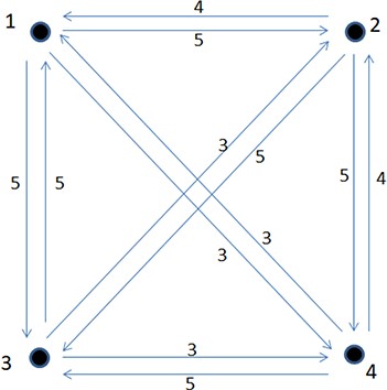
The directed weighted graph representing the interbank network that is used in the examples. The weights of the edges correspond to the exposures between the banks of the system.

Open in new tab Download slide

The present paper focuses on the study of the powerset |$2^X$| of the set |$X$|⁠, which contains all the possible combinations of defaulted banks. Since the set |$X$| of this example consists of |$4$| elements, the powerset |$2^X$| contains |$16$| sets. According to the approach of Section 3, each set |$A$| is usually identified with the indicator vector |$\boldsymbol{1_A} \in \mathbb{Z}_2^4$| with zero entries everywhere except the coordinates corresponding to the numbers belonging to |$A$|⁠. Our aim is to describe the contagion map |$T\colon \mathbb{Z}_2^n \to \mathbb{Z}_2^n$|⁠, the induced tree structure of |$2^X$|⁠, the matrix |$M_T$| and its canonical form and to calculate the contagion vector and the indicators |$m_1(T), m_2(T), m_3(T)$|⁠.

9.1 Example |$1$|

For our first example we take the value |$b = \frac{1}{10}$|⁠. This choice results in quite small bank capitals compared to the loans. Using the basic equation for the calculation of the contagion map |$T(\boldsymbol{1_A})= f(C-E_0 \cdot \boldsymbol{1_A})$| (see Proposition 3.1), we obtain, after some routine calculations, that the contagion map is given by

$$\begin{align*} &T(\emptyset) = \emptyset \quad \textrm{and} \quad T(A)=X \quad \textrm{for all}\ A\ne \emptyset.\end{align*}$$

Therefore, in this example the interbank system is extremely unstable and vulnerable and we have total contagion, that is the failure of any combination of banks results in the bankruptcy of all banks.

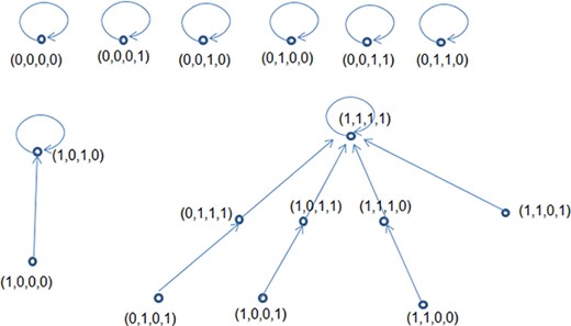
As it has been observed, in the case where we have total contagion, the powerset |$2^X$| contains only two maximal elements, namely the sets |$\emptyset = (0,0,0,0)$| and |$X=(1,1,1,1)$|⁠. Hence, the contagion graph |$2^X$| consists of two trees, as it is shown in Fig. 2.

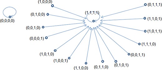
$The tree structure of $2^X \equiv \mathbb{Z}_2^4$ in the case of total contagion.$

Fig. 2.

The tree structure of |$2^X \equiv \mathbb{Z}_2^4$| in the case of total contagion.

Open in new tab Download slide

Using the function |$\varPhi $| and the procedure described in the beginning of Section 7, the contagion map |$T\colon \mathbb{Z}_2^4 \to \mathbb{Z}_2^4$| produces a linear operator |$S_T \colon \mathbb{R}^{16} \to \mathbb{R}^{16}$|⁠. In this case, we have |$S_T(e_0)=e_0$| and |$S_T(e_i)=e_{16}$| for any |$i=2,3,\ldots ,16$|⁠. Consequently, the |$16\times 16$|-matrix |$M_T$| is the following:

$$\begin{align*} &M_T= \left( \begin{array}{cccccccccccccccc} 1 & 0 & 0 & 0 & 0 & 0 & 0 & 0 & 0 & 0 & 0 & 0 & 0 & 0 & 0 & 0 \\ 0 & 0 & 0 & 0 & 0 & 0 & 0 & 0 & 0 & 0 & 0 & 0 & 0 & 0 & 0 & 0 \\ 0 & 0 & 0 & 0 & 0 & 0 & 0 & 0 & 0 & 0 & 0 & 0 & 0 & 0 & 0 & 0 \\ 0 & 0 & 0 & 0 & 0 & 0 & 0 & 0 & 0 & 0 & 0 & 0 & 0 & 0 & 0 & 0 \\ 0 & 0 & 0 & 0 & 0 & 0 & 0 & 0 & 0 & 0 & 0 & 0 & 0 & 0 & 0 & 0 \\ 0 & 0 & 0 & 0 & 0 & 0 & 0 & 0 & 0 & 0 & 0 & 0 & 0 & 0 & 0 & 0 \\ 0 & 0 & 0 & 0 & 0 & 0 & 0 & 0 & 0 & 0 & 0 & 0 & 0 & 0 & 0 & 0 \\ 0 & 0 & 0 & 0 & 0 & 0 & 0 & 0 & 0 & 0 & 0 & 0 & 0 & 0 & 0 & 0 \\ 0 & 0 & 0 & 0 & 0 & 0 & 0 & 0 & 0 & 0 & 0 & 0 & 0 & 0 & 0 & 0 \\ 0 & 0 & 0 & 0 & 0 & 0 & 0 & 0 & 0 & 0 & 0 & 0 & 0 & 0 & 0 & 0 \\ 0 & 0 & 0 & 0 & 0 & 0 & 0 & 0 & 0 & 0 & 0 & 0 & 0 & 0 & 0 & 0 \\ 0 & 0 & 0 & 0 & 0 & 0 & 0 & 0 & 0 & 0 & 0 & 0 & 0 & 0 & 0 & 0 \\ 0 & 0 & 0 & 0 & 0 & 0 & 0 & 0 & 0 & 0 & 0 & 0 & 0 & 0 & 0 & 0 \\ 0 & 0 & 0 & 0 & 0 & 0 & 0 & 0 & 0 & 0 & 0 & 0 & 0 & 0 & 0 & 0 \\ 0 & 0 & 0 & 0 & 0 & 0 & 0 & 0 & 0 & 0 & 0 & 0 & 0 & 0 & 0 & 0 \\ 0 & 1 & 1 & 1 & 1 & 1 & 1 & 1 & 1 & 1 & 1 & 1 & 1 & 1 & 1 & 1 \\ \end{array} \right) .\end{align*}$$

The Jordan canonical form of the matrix |$M_T$| can be derived immediately by the tree structure of Fig. 2. The Jordan canonical form consists of |$16$| Jordan blocks. Therefore, each block is a |$1\times 1$|-matrix. In other words, we have |$16$| linearly independent eigenvectors. More precisely, there are two linearly independent eigenvectors for the eigenvalue |$\lambda =1$| (because |$2^X$| contains two maximal elements), namely the vectors |$e_1$| and |$e_{16}$|⁠. There are also |$14$| linearly independent eigenvectors for the eigenvalue |$\lambda =0$|⁠, namely |$e_{16}-e_i$| for |$i=2,3,\ldots , 15$|⁠. The Jordan canonical form of |$M_T$| is the diagonal matrix that has two diagonal entries equal to |$1$| and the remaining |$14$| diagonal entries are |$0$|⁠.

Finally, by Proposition 4.1, the contagion vector is

$$\begin{align*} &V= (2^{4-1}-1) \textbf{1} = (7,7,7,7),\end{align*}$$

and by Example 4.2, we know that

$$\begin{align*} &m_1(T) = m_2(T) =m_3(T)=1.\end{align*}$$

9.2 Example |$2$|

For our second example, we set |$b=10$| and the vector of capitals becomes

$$\begin{align*} &C = \left( \begin{array}{c} 70 \\ 70 \\ 30 \\ 80 \\ \end{array} \right). \end{align*}$$

In this case, the capitals are quite large compared to the loans and the system is expected to be robust. Indeed, by Proposition 3.1, we can easily see that the contagion map is

$$\begin{align*} &T(\boldsymbol{1_A}) =\boldsymbol{1_A} \quad \textrm{for all}\ A\in 2^X.\end{align*}$$

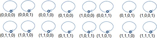
$The tree structure of $2^X \equiv \mathbb{Z}_2^4$ in the case where there is no contagion.$

Fig. 3.

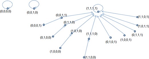
The tree structure of |$2^X \equiv \mathbb{Z}_2^4$| in the case where there is no contagion.

Open in new tab Download slide

$$\begin{align*} &V=(0,0,0,0) \quad \textrm{and} \quad m_1(T) = m_2(T) =m_3(T)=0.\end{align*}$$

9.3 Example |$3$|

In the third example, we consider some case in the middle of the two extreme cases described in the previous examples. The value |$b=1$| results in the vector of capitals

$$\begin{align*} &C = \left( \begin{array}{c} 7 \\ 7 \\ 3 \\ 8 \\ \end{array} \right). \end{align*}$$

Using Proposition 3.1, we obtain, after routine calculations, that the contagion map |$T\colon \mathbb{Z}_2^4 \to \mathbb{Z}_2^4$| is the following:

$$\begin{align*} T(0,0,0,0) = (0,0,0,0) \quad & \quad T(0,1,1,0) = (1,1,1,1) \\ T(0,0,0,1) = (0,0,1,1) \quad & \quad T(1,0,1,0) = (1,1,1,1) \\ T(0,0,1,0) = (0,0,1,0) \quad & \quad T(1,1,0,0) = (1,1,1,0) \\ T(0,1,0,0) = (0,1,1,0) \quad & \quad T(0,1,1,1) = (1,1,1,1) \\ T(1,0,0,0) = (1,0,1,0) \quad & \quad T(1,0,1,1) = (1,1,1,1) \\ T(0,0,1,1) = (1,1,1,1) \quad & \quad T(1,1,0,1) = (1,1,1,1) \\ T(0,1,0,1) = (1,1,1,1) \quad & \quad T(1,1,1,0) = (1,1,1,1) \\ T(1,0,0,1) = (1,1,1,1) \quad & \quad T(1,1,1,1) = (1,1,1,1) .\end{align*}$$

The above contagion map |$T$| generates the tree structure of the contagion graph |$2^X \equiv \mathbb{Z}_2^4$| shown in Fig. 4.

$The tree structure of $2^X \equiv \mathbb{Z}_2^4$.$

Fig. 4.

The tree structure of |$2^X \equiv \mathbb{Z}_2^4$|⁠.

Open in new tab Download slide

We observe that there are three maximal elements, namely |$(0,0,0,0)$|⁠, |$(0,0,1,0)$| and |$(1,1,1,1)$| and thus |$\mathbb{Z}_2^4$| consists of three connected components.

Using the function |$\varPhi \colon \mathbb{Z}_2^4 \to (e_i)_{i=1}^{16}$| a linear operator |$S_T\colon \mathbb{R}^{16} \to \mathbb{R}^{16}$| is produced. The corresponding |$16\times 16$|-matrix |$M_T$| is the following:

$$\begin{align*} &M_T= \left( \begin{array}{cccccccccccccccc} 1 & 0 & 0 & 0 & 0 & 0 & 0 & 0 & 0 & 0 & 0 & 0 & 0 & 0 & 0 & 0 \\ 0 & 0 & 0 & 0 & 0 & 0 & 0 & 0 & 0 & 0 & 0 & 0 & 0 & 0 & 0 & 0 \\ 0 & 0 & 1 & 0 & 0 & 0 & 0 & 0 & 0 & 0 & 0 & 0 & 0 & 0 & 0 & 0 \\ 0 & 0 & 0 & 0 & 0 & 0 & 0 & 0 & 0 & 0 & 0 & 0 & 0 & 0 & 0 & 0 \\ 0 & 0 & 0 & 0 & 0 & 0 & 0 & 0 & 0 & 0 & 0 & 0 & 0 & 0 & 0 & 0 \\ 0 & 1 & 0 & 0 & 0 & 0 & 0 & 0 & 0 & 0 & 0 & 0 & 0 & 0 & 0 & 0 \\ 0 & 0 & 0 & 0 & 0 & 0 & 0 & 0 & 0 & 0 & 0 & 0 & 0 & 0 & 0 & 0 \\ 0 & 0 & 0 & 0 & 0 & 0 & 0 & 0 & 0 & 0 & 0 & 0 & 0 & 0 & 0 & 0 \\ 0 & 0 & 0 & 1 & 0 & 0 & 0 & 0 & 0 & 0 & 0 & 0 & 0 & 0 & 0 & 0 \\ 0 & 0 & 0 & 0 & 1 & 0 & 0 & 0 & 0 & 0 & 0 & 0 & 0 & 0 & 0 & 0 \\ 0 & 0 & 0 & 0 & 0 & 0 & 0 & 0 & 0 & 0 & 0 & 0 & 0 & 0 & 0 & 0 \\ 0 & 0 & 0 & 0 & 0 & 0 & 0 & 0 & 0 & 0 & 0 & 0 & 0 & 0 & 0 & 0 \\ 0 & 0 & 0 & 0 & 0 & 0 & 0 & 0 & 0 & 0 & 0 & 0 & 0 & 0 & 0 & 0 \\ 0 & 0 & 0 & 0 & 0 & 0 & 0 & 0 & 0 & 0 & 0 & 0 & 0 & 0 & 0 & 0 \\ 0 & 0 & 0 & 0 & 0 & 0 & 0 & 0 & 0 & 0 & 1 & 0 & 0 & 0 & 0 & 0 \\ 0 & 0 & 0 & 0 & 0 & 1 & 1 & 1 & 1 & 1 & 0 & 1 & 1 & 1 & 1 & 1 \\ \end{array} \right) .\end{align*}$$

The characteristic polynomial of |$M_T$| is |$(1-x)^{13}(-x)^3$|⁠. The Jordan canonical form of |$M_T$| can be obtained directly from Fig. 4. Indeed, the three maximal elements produce three linearly independent eigenvector for the eigenvalue |$\lambda =1$|⁠. The minimal elements |$(0,0,0,1)$|⁠, |$(0,1,0,0)$|⁠, |$(1,0,0,0)$| and |$(1,1,0,0)$| produce |$2\times 2$| Jordan blocks for the eigenvalue |$\lambda =0$|⁠. The remaining minimal elements give Jordan blocks for |$\lambda =0$| of dimension |$1\times 1$|⁠. Hence, the Jordan canonical form of |$M_T$| is

$$\begin{align*} &J_M= \left( \begin{array}{cccccccccccc} J_1 & & & & & & & & & & & \\ & J_2 & & & & & & & & & & \\ & & J_3 & & & & & & & & & \\ & & & J_4 & & & & & & & & \\ & & & & J_5 & & & & & & & \\ & & & & & J_6 & & & & & & \\ & & & & & & J_7 & & & & & \\ & & & & & & & J_8 & & & & \\ & & & & & & & & J_9 & & & \\ & & & & & & & & & J_{10} & & \\ & & & & & & & & & & J_{11} & \\ & & & & & & & & & & & J_{12} \\ \end{array} \right) .\end{align*}$$

where |$J_i=(1)$| for |$i=1,2,3$|⁠, |$J_i=(0)$| for |$i=4,5,6,7,8$| and

$$\begin{align*} &J_i = \left( \begin{array}{cc} 0 & 1 \\ 0 & 0 \end{array} \right) \end{align*}$$

for |$i=9,10,11,12$|⁠.

We proceed now with the calculation of contagion vector. By Equation (4.1), this vector is given by |$V=\sum _{A\in 2^X} (\boldsymbol{1_{T(A)}} - \boldsymbol{1_A})$|⁠. However, from the analysis of Section 5, we obtain that

$$\begin{align*} V= \sum_{A\ \textrm{maximal}} \sum_{D\in P_A} (1_{T(D)}-1_D) = \sum_{D\in P_{X}} (1_{T(D)}-1_D) = \sum_{i=1}^9 (1_{X}-1_{B_i}), \end{align*}$$

where |$(B_i)_{i=1}^9$| are the minimal elements belonging to the connected component |$P_X$|⁠. An easy calculation shows that

$$\begin{align*} &V = (4,4,7,3).\end{align*}$$

As it was expected the entry corresponding to the third bank is quite large, since this bank has the least capital of all. Now, we can easily obtain the indicators. By Propositions 4.2 and 4.3, we have

$$\begin{align*} &m_1(T) = \frac{\left\langle V, \textbf{1} \right\rangle}{4\cdot (2^3 -1)} = \frac{4+4+7+3}{28}=\frac{18}{28}=\frac{9}{14} \approx 0.643.\end{align*}$$

$$\begin{align*} &m_2(T) = \frac{\left\langle V, C \right\rangle}{(2^3 -1)\left\langle \textbf{1},C \right\rangle} = \frac{4\cdot 7 + 4\cdot 7 +7\cdot 3+3\cdot 8}{7\cdot (7+7+3+8)}=\frac{101}{175} \approx 0.577.\end{align*}$$

$$\begin{align*} &m_3(T) = \frac{\left\langle V, L \right\rangle}{(2^3 -1)\left\langle \textbf{1},L \right\rangle} = \frac{4\cdot 12 + 4\cdot 12+7\cdot 15+3\cdot 11}{7\cdot (12+12+15+11)}=\frac{234}{350} \approx 0.669.\end{align*}$$

9.4 Example |$4$|

The tree structure of Fig. 4 indicates that the interbank system of the third example is still quite prone to financial contagion. For this reason, we increase now the value of |$b$| to |$\frac{3}{2}$|⁠. Thus the vector of capitals becomes

$$\begin{align*} &C = \left( \begin{array}{c} 10.5 \\ 10.5 \\ 4.5 \\ 12 \\ \end{array} \right). \end{align*}$$

The system is expected now to be more stable. Indeed, the contagion map |$T\colon \mathbb{Z}_2^4 \to \mathbb{Z}_2^4$| is the following:

$$\begin{align*} T(0,0,0,0) = (0,0,0,0) \quad & \quad T(0,1,1,0) = (0,1,1,0) \\ T(0,0,0,1) = (0,0,0,1) \quad & \quad T(1,0,1,0) = (1,0,1,0) \\ T(0,0,1,0) = (0,0,1,0) \quad & \quad T(1,1,0,0) = (1,1,1,0) \\ T(0,1,0,0) = (0,1,0,0) \quad & \quad T(0,1,1,1) = (1,1,1,1) \\ T(1,0,0,0) = (1,0,1,0) \quad & \quad T(1,0,1,1) = (1,1,1,1) \\ T(0,0,1,1) = (0,0,1,1) \quad & \quad T(1,1,0,1) = (1,1,1,1) \\ T(0,1,0,1) = (0,1,1,1) \quad & \quad T(1,1,1,0) = (1,1,1,1) \\ T(1,0,0,1) = (1,0,1,1) \quad & \quad T(1,1,1,1) = (1,1,1,1) .\end{align*}$$

The map |$T$| imposes on |$2^X$| the tree structure presented in Fig. 5. We observe that there are eight maximal sets and |$2^X$| consists of eight connected components.

$The tree structure of $2^X \equiv \mathbb{Z}_2^4$ for the fourth example.$

Fig. 5.

The tree structure of |$2^X \equiv \mathbb{Z}_2^4$| for the fourth example.

Open in new tab Download slide

The generated matrix |$M_T$| is the following:

$$\begin{align*} &M_T= \left( \begin{array}{cccccccccccccccc} 1 & 0 & 0 & 0 & 0 & 0 & 0 & 0 & 0 & 0 & 0 & 0 & 0 & 0 & 0 & 0 \\ 0 & 1 & 0 & 0 & 0 & 0 & 0 & 0 & 0 & 0 & 0 & 0 & 0 & 0 & 0 & 0 \\ 0 & 0 & 1 & 0 & 0 & 0 & 0 & 0 & 0 & 0 & 0 & 0 & 0 & 0 & 0 & 0 \\ 0 & 0 & 0 & 1 & 0 & 0 & 0 & 0 & 0 & 0 & 0 & 0 & 0 & 0 & 0 & 0 \\ 0 & 0 & 0 & 0 & 0 & 0 & 0 & 0 & 0 & 0 & 0 & 0 & 0 & 0 & 0 & 0 \\ 0 & 0 & 0 & 0 & 0 & 1 & 0 & 0 & 0 & 0 & 0 & 0 & 0 & 0 & 0 & 0 \\ 0 & 0 & 0 & 0 & 0 & 0 & 0 & 0 & 0 & 0 & 0 & 0 & 0 & 0 & 0 & 0 \\ 0 & 0 & 0 & 0 & 0 & 0 & 0 & 0 & 0 & 0 & 0 & 0 & 0 & 0 & 0 & 0 \\ 0 & 0 & 0 & 0 & 0 & 0 & 0 & 0 & 1 & 0 & 0 & 0 & 0 & 0 & 0 & 0 \\ 0 & 0 & 0 & 0 & 1 & 0 & 0 & 0 & 0 & 1 & 0 & 0 & 0 & 0 & 0 & 0 \\ 0 & 0 & 0 & 0 & 0 & 0 & 0 & 0 & 0 & 0 & 0 & 0 & 0 & 0 & 0 & 0 \\ 0 & 0 & 0 & 0 & 0 & 0 & 1 & 0 & 0 & 0 & 0 & 0 & 0 & 0 & 0 & 0 \\ 0 & 0 & 0 & 0 & 0 & 0 & 0 & 1 & 0 & 0 & 0 & 0 & 0 & 0 & 0 & 0 \\ 0 & 0 & 0 & 0 & 0 & 0 & 0 & 0 & 0 & 0 & 0 & 0 & 0 & 0 & 0 & 0 \\ 0 & 0 & 0 & 0 & 0 & 0 & 0 & 0 & 0 & 0 & 1 & 0 & 0 & 0 & 0 & 0 \\ 0 & 0 & 0 & 0 & 0 & 0 & 0 & 0 & 0 & 0 & 0 & 1 & 1 & 1 & 1 & 1 \\ \end{array} \right). \end{align*}$$

The characteristic polynomial of |$M_T$| is |$(1-x)^8(-x)^8$|⁠. The Jordan canonical form of |$M_T$| is as follows: the maximal elements of |$2^X$| generate linearly independent eigenvector for the eigenvalue |$\lambda =1$|⁠. Hence, we have eight Jordan blocks of the form |$J_i=(1)$| for |$i=1,2,\ldots , 8$|⁠. The minimal elements |$(0,1,0,1)$|⁠, |$(1,0,0,1)$| and |$(1,1,0,0)$| produce Jordan blocks of dimensions |$2\times 2$| for the eigenvalue |$\lambda =0$|⁠. That is, we have

$$\begin{align*} &J_i = \left( \begin{array}{cc} 0 & 1 \\ 0 & 0 \end{array} \right) \quad \textrm{for}\ i=9,10,11. \end{align*}$$

Finally, the minimal elements |$(1,1,0,1)$| and |$(1,0,0,0)$| generate |$1\times 1$| Jordan blocks for the eigenvalue |$\lambda =0$|⁠. That is, |$J_i=(0)$| for |$=12,13$|⁠.

Using the calculations of Section 5, we find that the contagion vector is given by

$$\begin{align*} V= \sum_{A\ \textrm{maximal}} \sum_{D\in P_A} (1_{T(D)}-1_D)& = \sum_{D\in P_{(1,0,1,0)}}(1_{T(D)}-1_D)+\sum_{D\in P_{(1,1,1,1)}} (1_{T(D)}-1_D)\\ &= (1,0,1,0) + \sum_{j=1}^4 ((1,1,1,1)-1_{B_j}), \end{align*}$$

where |$(B_j)_{j=1}^4$| are the minimal elements of the component |$P_{(1,1,1,1)}$|⁠. Now, it follows easily that

$$\begin{align*} &V = (1,1,5,1).\end{align*}$$

The contagion vector shows that the situation of every bank has improved compared to the third example. However, the third bank is still in difficult position, and the reason is that its capital is not big enough in relation to its loans.

Finally, the indicators for the interbank system of the present example are given below

$$\begin{align*} &m_1(T) = \frac{\left\langle V, \textbf{1} \right\rangle}{4\cdot (2^3 -1)} = \frac{1+1+5+1}{28}=\frac{8}{28}=\frac{2}{7} \approx 0.286.\end{align*}$$

$$\begin{align*} &m_2(T) = \frac{\left\langle V, C \right\rangle}{(2^3 -1)\left\langle \textbf{1},C \right\rangle} = \frac{1\cdot 7 + 1\cdot 7 +5\cdot 3+1\cdot 8}{7\cdot (7+7+3+8)}=\frac{37}{175} \approx 0.211.\end{align*}$$

$$\begin{align*} &m_3(T) = \frac{\left\langle V, L \right\rangle}{(2^3 -1)\left\langle \textbf{1},L \right\rangle} = \frac{1\cdot 12 + 1\cdot 12+5\cdot 15+1\cdot 11}{7\cdot (12+12+15+11)}=\frac{110}{350} \approx 0.314.\end{align*}$$

9.5 Summary

The next matrix summarizes the contagion vector and the indicators for all the above examples:

$$\begin{align*} & \begin{array}{|c|c|c|c|c|} \hline & \textrm{Example}\ 1 & \textrm{Example}\ 3 & \textrm{Example}\ 4 & \textrm{Example}\ 2 \\ \hline V & (7,7,7,7) & (4,4,7,3) & (1,1,5,1) & (0,0,0,0) \\ \hline m_1(T) & 1 & 0.643 & 0.286 & 0 \\ \hline m_2(T) & 1 & 0.577 & 0.211 & 0 \\ \hline m_3(T) & 1 & 0.669 & 0.314 & 0 \\ \hline \end{array} \end{align*}$$

It can be seen that when |$b=1$| (Example |$3$|⁠) then the coordinates of the contagion vector are quite large and so are the indicators |$m_1, m_2, m_3$|⁠. Therefore, the banks belonging to the system are vulnerable and the whole network is unstable and prone to financial contagion. Any initial shock can trigger a series of defaults and it causes severe damage.

On the contrary, when |$b=\frac{3}{2}$| (Example |$4$|⁠) the situation has improved drastically. Excluding the third bank, the others are quite robust and show resilience to financial shocks. Therefore, the value |$b=\frac{3}{2}$| represents a threshold that the network should cross in order to achieve a satisfying level of robustness.

The third bank is the most vulnerable of the network. Even when the situation of the other banks has improved, the bank |$3$| continues to be at risk. Consequently, this bank should consider additional measures in order to become more robust. These measures may include capital raise or loans reduction or a combination of both policies.

10. Final conclusions: assessment of banks and networks and formulation of policies

The present paper is oriented towards the study of financial contagion in an interbank network system. In order to describe this problem and analyse its parameters, we developed theoretical models that are inspired by tools and techniques coming from dynamical systems and operator theory. However, our ultimate goal is to propose various methods that, given an arbitrary network, enable the assessment of the network as a whole and of each individual institution of which the network consists. As a result, they facilitate the regulators and policy makers in the most suitable decision making. In this last section, aiming at people working in the interbank sector, we wish to isolate and highlight the most important of our results concerning assessment and formulation of policies.

10.1 Assessment of individual banks

Our main tool for evaluating any individual bank of the network is the contagion vector |$V$| (see equation (4.1)). Indeed, as we have commented earlier (see Sections 4 and 9), the values of the coordinates of |$V$| measure the robustness of the corresponding banks. If a coordinate is large, then the corresponding bank is prone to financial shocks. On the contrary, the institutions that correspond to the smallest entries of |$V$| are the most stable and they show resilience to financial shocks.

Furthermore, in order to assess the importance of each bank for the whole network, we can appeal to the maximal chains |$\mathcal{C}_i$|⁠, |$i=1,2,\ldots ,n$|⁠. Recall from Section 2 that the chains |$\mathcal{C}_i$| are defined as follows: for any |$i=1,2,\ldots ,n$|⁠, we have

$$\begin{align*} &\mathcal{C}_i = \{ \{i\}, T(\{i\}), T^2(\{i\}), \ldots, T^{n_i}(\{i\}) \},\end{align*}$$

where |$T^{n_i}(\{i\})$| is an equilibrium set, that is |$T^{n_i+1}(\{i\})=T^{n_i}(\{i\})$|⁠. The cardinality of the set |$T^{n_i}(\{i\})$| shows how many banks are affected by the failure of the bank |$i$| and, clearly, the bigger it is the more important the bank. For instance, there are two extreme cases. The first one occurs when the cardinality of |$T^{n_i}(\{i\})$| is equal to |$1$|⁠. This means that no other bank is affected by the default of the bank |$i$|⁠. Hence, this bank is almost unimportant for the network. The second extreme case is when |$\sharp T^{n_i}(\{i\})=\sharp X$|⁠, which implies that the bank is vital for the network, as its default leads to the collapse of the whole network.

The second crucial feature of the chain |$\mathcal{C}_i$|⁠, which should be considered in connection to the previous one, is the time that intervenes between the initial shock and the point where the contagion stops and it can be measured by the length |$n_i$| of the chain. The size of this period of time plays an essential role to the strategies that should be considered in order to reduce the contagion effects.

10.2 Assessment of the network

In order to assess the robustness of an interbank network, we have defined three indicators |$m_1, m_2, m_3$| (see Section 4). These quantities take values between |$0$| and |$1$| and measure the level of the contagion in the whole network. The closest to |$0$| they are, the more stable the network. In such a case, the default of each and every bank has limited consequences for the system, which reaches a solid situation relatively quickly. On the contrary, when the indicators are close to |$1$|⁠, the system is very unstable and is prone to financial contagion.

Furthermore, the indicators measure the total damage, i.e. the losses that the system might experience given all possible choices of initially defaulted entities. More precisely, the indicator |$m_1$| estimates the proportion of the affected banks. The second and third indicators measure the capitals that are destroyed and the loans that are not paid back, respectively. Additionally, it should be highlighted that these indicators on the one hand evaluate the network and, on the other hand, make possible the comparison of different networks even though they are completely disjoint from each other.

10.3 Understanding and supervision of systemic risk in an interbank network

Having made the aforementioned assessments, the regulators and supervisors of the interbank network will be able to propose corrective actions and measures (the least possible) in order to improve the resilience of the network to systemic shocks. For instance, the contagion vector assess the vulnerability of each bank belonging to the network and classify them from the most powerful to the most vulnerable. As a consequence, the supervisors are able to detect the weak points of the interbank system and to take suitable proactive measures.

The most important feature in the present work is that we study the contagion in a specific network without using simulation. Our purpose is not to locate and explain the sources of financial contagion in an interbank system in general. On the contrary, our results develop a generic method that in an arbitrary network specifies the properties of the network and the banks of which it consists and their behaviour to financial shocks. Consequently, the ideas and work included in this article actually propose a working methodology for the regulators and supervisors of an interbank network. This methodology consists of three steps.

STEP 1: The starting point is to depict the interbank network that is going to be studied and evaluated. This means that at the particular time the bank institutions participating in the network should be recorded as well as the capital possessed by each bank and the lending relationships among them.

STEP 3: Once the contagion graph has been constructed, the supervisors and regulators of the network, using the methods introduced in this paper, will be able to perform the following tasks:

To assess the vulnerability of any specific bank or of any specific set of banks.
To estimate the vulnerability of the whole network and to detect its weakest points.
To classify the banks of the system according to their vulnerability.
To introduce new metrics and indicators. Clearly, the aforementioned assessments can be achieved through the indicators that are proposed in the paper, which are the most fundamental and typical. However, one may consider new indicators shedding light into different aspects of the network.
To alter the initial conditions (capital, loans, interconnectedness) and to examine the development of crises under various scenarios. Therefore, the regulator will be able to study the consequences of any changes in the initial network and to choose the most appropriate of them.

To summarise, through the present work, the regulator of an interbank network will be able to study the transmission of an economic crisis, to reveal the strong and weak points of the network, to classify the banks or parts of the networks according with their vulnerability and to examine several scenarios.

Acknowledgements

The authors would like to thank the anonymous referees for their helpful remarks.

References

Acemoglu

Ozdaglar

Tahbaz-Salehi

(

2015

)

Systemic risk and stability in financial networks

Am. Econ. Rev.

105

564

–

608

Allen

Gale

(

2000

)

Financial contagion

J. Polit. Econ.

108

–

Google Scholar

Crossref

WorldCat

Amini

Cont

Minca

(

2016

)

Resilience to contagion in financial networks

Math. Finance

329

–

365

Google Scholar

Crossref

WorldCat

Anand

Craig

Von Peter

(

2015

)

Filling in the blanks: network structure and interbank contagion

Quant. Finance

625

–

636

Anderson

(

1985

)

Combinatorics of Finite Sets

Oxford

Science Publications

Google Scholar

Google Preview

OpenURL Placeholder Text

WorldCat

Bardoscia

Battiston

Caccioli

Caldarelli

(

2017

)

Pathways towards instability in financial networks

Nat. Commun.

14416

. doi:10.1038/ncomms14416.

Barucca

Bardoscia

Caccioli

D’Errico

Visentin

Battiston

Caldarelli

(

2016

)

Network Valuation in Financial Systems

. Available at SSRN: https://ssrn.com/abstract=2795583 or http://dx.doi.org/10.2139/ssrn.2795583

Battiston

Puliga

Kaushik

Tasca

Caldarelli

(

2012

)

Debtrank: too central to fail? Financial networks, the fed and systemic risk

Sci. Rep.

541

Caccioli

Catanach

T. A.

Farmer

J. D.

(

2012

)

Heterogeneity, correlations and financial contagion

Adv. Complex Syst.

No. supp02

Caccioli

Shrestha

Moore

Farmer

(

2014

)

Stability analysis of financial contagion due to overlapping portfolios

J. Bank. Financ.

233

–

245

Google Scholar

Crossref

WorldCat

Chinazzi

Pegoraro

Fagiolo

(

2015

)

Defuse the bomb: rewiring interbank networks

LEM Working Paper Series

Institute of Economics, Scuola Superiore Sant’ Anna

Cifuentes

Shin

H. S.

Ferrucci

(

2005

)

Liquidity risk and contagion

J. Eur. Econ. Assoc.

556

–

566

Google Scholar

Crossref

WorldCat

Cimini

Squartini

Garlaschelli

Gabrielli

(

2015

)

Systemic risk analysis on reconstructed economic and financial networks

Sci. Rep.

15758

Cont

Moussa

Santos

E. B.

(

2010

)

Network Structure and Systemic Risk in Banking Systems

. Available at SSRN: https://ssrn.com/abstract=1733528 or http://dx.doi.org/10.2139/ssrn.1733528

De Souza

S. R. S.

Silva

T. C.

Tabak

B. M.

Guerra

S. M.

(

2016

)

Evaluating systemic risk using bank default probabilities in financial networks

J. Econom. Dynam. Control

–

Google Scholar

Crossref

WorldCat

Elliott

Golub

Jackson

M.O.

(

2014

)

Financial networks and contagion

Am. Econ. Rev.

104

3115

–

3153

Google Scholar

Crossref

WorldCat

Elsinger

Lehar

Summer

(

2006

)

Risk assessment for banking systems

Manage. Sci.

1301

–

1314

Google Scholar

Crossref

WorldCat

Fink

Krüger

Meller

Wong

L.-H.

(

2016

)

The credit quality channel: modeling contagion in the interbank market

J. Finan. Stab.

–

Google Scholar

Crossref

WorldCat

Freixas

Parigi

B.M.

Rochet

J.-C.

(

2000

)

Systemic risk, interbank relations, and liquidity provision by the central bank

J. Money Credit Bank.

611

–

638

Google Scholar

Crossref

WorldCat

Gai

Kapadia

(

2010

)

Contagion in financial networks

P. Roy. Soc. A-Math. Phy.

466

2401

–

2423

Google Scholar

OpenURL Placeholder Text

WorldCat

Galbiati

Delpini

Battiston

(

2013

)

The power to control

Nature Phys.

126

–

128

Google Scholar

Crossref

WorldCat

Gandy

Veraart

L.A.

(

2016

)

A bayesian methodology for systemic risk assessment in financial networks

Manage. Sci.

4428

–

4446

Google Scholar

Crossref

WorldCat

Georgescu

O.-M.

(

2015

)

Contagion in the interbank market: funding versus regulatory constraints

J. Finan. Stab.

–

Google Scholar

Crossref

WorldCat

Glasserman

Young

H. P.

(

2015

)

How likely is contagion in financial networks

J. Bank. Financ.

383

–

339

Google Scholar

Crossref

WorldCat

Glasserman

Young

H.P.

(

2016

)

Contagion in financial networks

J. Econ. Lit.

779

–

831

Google Scholar

Crossref

WorldCat

Greenwood

Landier

Thesmar

(

2015

)

Vulnerable banks

J. Financ. Econ.

115

471

–

485

Google Scholar

Crossref

WorldCat

Hałaj

Kok

(

2013

)

Assessing interbank contagion using simulated networks

Comput. Manag. Sci.

157

–

186

Google Scholar

Crossref

WorldCat

Huang

Zhou

Zhu

(

2012

)

Assessing the systemic risk of a heterogeneous portfolio of banks during the recent financial crisis

J. Finan. Stab.

193

–

205

Google Scholar

Crossref

WorldCat

Iori

Jafarey

Padilla

(

2006

)

Systemic risk on the interbank market

J. Econ. Behav. Organ.

525

–

542

Google Scholar

Crossref

WorldCat

Karcanias

Koivo

H. N.

Kyriakopoulos

(

1995

)

Systems, modelling and control theory issues in global operation of industrial processes

IFAC Proc. Vol.

221

–

228

Google Scholar

Crossref

WorldCat

Ladley

(

2013

)

Contagion and risk-sharing on the inter-bank market

J. Econom. Dynam. Control

1384

–

1400

Google Scholar

Crossref

WorldCat

Leventides

Loukaki

Papavassiliou

V. G.

(

2019

)

Simulating financial contagion dynamics in random interbank networks

J. Econ. Behav. Organ.

158

500

–

525

Google Scholar

Crossref

WorldCat

Memmel

Sachs

(

2013

)

Contagion in the interbank market and its determinants

J. Finan. Stab.

–

Google Scholar

Crossref

WorldCat

Mistrulli

P.E.

(

2011

)

Assessing financial contagion in the interbank market: maximum entropy versus observed interbank lending patterns

J. Bank. Financ.

1114

–

1127

Google Scholar

Crossref

WorldCat

Nier

Yang

Yorulmazer

Alentorn

(

2007

)

Network models and financial stability

J. Econom. Dynam. Control

2033

–

2060

Google Scholar

Crossref

WorldCat

Tonzer

(

2015

)

Cross-border interbank networks, banking risks and contagion

J. Finan. Stab.

–

Google Scholar

Crossref

WorldCat

Upper

(

2011

)

Simulation methods to assess the danger of contagion in interbank markets

J. Finan. Stab.

111

–

125

Google Scholar

Crossref

WorldCat

This is an Open Access article distributed under the terms of the Creative Commons Attribution License (https://creativecommons.org/licenses/by/4.0/), which permits unrestricted reuse, distribution, and reproduction in any medium, provided the original work is properly cited.

Download all slides

Month:	Total Views:
April 2021	18
May 2021	17
June 2021	1
July 2021	3
August 2021	3
October 2021	10
November 2021	14
December 2021	12
January 2022	17
February 2022	17
March 2022	73
April 2022	25
May 2022	11
June 2022	42
July 2022	40
August 2022	15
September 2022	18
October 2022	12
November 2022	27
December 2022	19
January 2023	11
February 2023	25
March 2023	10
April 2023	20
May 2023	14
June 2023	4
July 2023	9
August 2023	12
September 2023	14
October 2023	27
November 2023	24
December 2023	13
January 2024	12
February 2024	28
March 2024	10
April 2024	12
May 2024	9
June 2024	15
July 2024	13
August 2024	8
September 2024	5
October 2024	6
November 2024	4
December 2024	2
January 2025	9
February 2025	7
March 2025	10
April 2025	4
May 2025	3

Article Contents

A discrete dynamics approach to interbank financial contagion

Abstract

1. Introduction

2. Mathematical modelling of interbank networks and financial contagion

2.1 The interbank network and default contagion

2.2 The contagion map

2.3 The contagion relation

2.4 Maximal and minimal elements of |$(2^X,\leqslant ^c)$|

2.5 Chains and circles of |$(2^X, \leqslant ^c)$|

2.6 Connected components and the tree-structure of |$(2^X, \leqslant ^c)$|

3. Boolean dynamical systems

4. Quantitative analysis of the contagion

4.1 The contagion vector

4.2 Indicators

5. Calculation of the contagion vector and the indicators

6. Upper and lower bounds

6.1 Lower bound

6.2 Upper bound

7. Description through linear operators

7.1 Contagion vector and linear operator

8. The eigenstructure of the matrix |$M_T$|

9. Examples

9.1 Example |$1$|

9.2 Example |$2$|

9.3 Example |$3$|

9.4 Example |$4$|

9.5 Summary

10. Final conclusions: assessment of banks and networks and formulation of policies

10.1 Assessment of individual banks

10.2 Assessment of the network

10.3 Understanding and supervision of systemic risk in an interbank network

Acknowledgements

References

Citations

Views

Altmetric

Email alerts

Citing articles via

Latest

Most Read

Most Cited

This Feature Is Available To Subscribers Only