Abstract
We introduce the concept of |$\epsilon $|-uncontrollability for random linear systems, i.e. linear systems in which the usual matrices have been replaced by random matrices. We also estimate the |$\varepsilon $|-uncontrollability in the case where the matrices come from the Gaussian orthogonal ensemble. Our proof utilizes tools from systems theory, probability theory and convex geometry.
1. Introduction
Controllability is one of the most fundamental concepts in systems theory and control theory. Roughly speaking, a system is controllable if one can switch from one trajectory to the other provided that the laws governing the system are obeyed and some delay is allowed. In the present work, we focus on the linear, time-invariant multivariable system described by the following equations (
Karkanias & Milonidis, 2007;
Polderman & Willems, 1998):
where
|$\textbf{x}=\textbf{x}(t)=(x_1(t), x_2(t), \ldots , x_n(t))^t\in \mathbb{R}^n$| is a vector describing the state of the system at time
|$t$|,
|$\textbf{u}=u(t)\in \mathbb{R}$| is the input and
|$\textbf{y}=y(t)$| is the
|$m$|-vector of outputs.
|$\textbf{A}$|,
|$\textbf{C}$| are
|$n\times n$|,
|$m\times n$| matrices, respectively, and
|$\textbf{b}\in \mathbb{R}^n$|,
|$\textbf{d}\in \mathbb{R}^m$| are vectors. In this case, the definition of controllability goes as follows. System (
1.1) is said to be
state controllable or simply
controllable if there exists a finite time
|$T>0$|, such that for any initial state
|$\textbf{x}(0)\in \mathbb{R}^n$| and any
|$\textbf{x}_{\textbf{1}}\in \mathbb{R}^n$|, there is an input
|$\textbf{u}=u(t)$| defined on
|$[0,T]$| that will transfer
|$\textbf{x}(0)$| to
|$\textbf{x}_{\textbf{1}}$| at time
|$T$| (i.e.
|$\textbf{x}(t)$| obeys the first equation of (
1.1) and
|$\textbf{x}(T)=\textbf{x}_{\textbf{1}}$|). Otherwise, the system (
1.1) is called
uncontrollable.
In this article, we consider random systems of the form (1.1), i.e. systems where the parameters |$\textbf{A}$| and |$\textbf{b}$| have been replaced with random matrices. Given a positive number |$\epsilon $|, we define the concept of |$\epsilon $|-uncontrollability of a random system. It is natural that the |$\epsilon $|-uncontrollability of a random system depends on the distribution of the entries of |$\textbf{A}$| and |$\textbf{b}$|. Consequently, we consider the fundamental Gaussian orthogonal ensemble (GOE)of random matrices and we calculate the |$\epsilon $|-uncontrollability in this particular case. Controllability of random linear systems has also been studied in O’Rourke & Touri, 2015. However, the present work has a different purpose on this issue.
The rest of the paper is organized as follows. In Section 2, we define the |$\epsilon $|-uncontrollability for random systems. In Section 3, we describe the GOE, which is going to be used in this work and we state some known results about this ensemble that will be exploited in the sequel. In Section 4, we consider the case |$n=2$|, i.e. when the state space is |$\mathbb{R}^2$|, and we give the detailed calculation of the |$\epsilon $|-uncontrollability of a random system where the matrix |$\textbf{A}$| comes from the GOE. Finally, in Section 5, we deal with the general case of |$\mathbb{R}^n$| for |$n>2$|. In this case, the situation is more complicated and we provide upper and lower bounds for the |$\epsilon $|-uncontrollability of a random system.
We close this introductory section with some comments concerning the motivation of the present work. Random matrix theory applies in problems of algebraic control in the presence of error or noise due to many factors. Here, we ignore systematic errors and we consider the effect of randomness to algebraic relations (equalities). For example, suppose that a set of equations
|$\textbf{f}(\textbf{x})=0$| is given. In order to study the effect of a random perturbation
|$\textbf{x}+\varepsilon \textbf{p}$|, where
|$\textbf{x}$| is a given solution and
|$\textbf{p}$| is a random variable, we expand
|$\textbf{f}(\textbf{x}+\varepsilon \textbf{p})$| into
and we examine the statistical properties of
|$\textbf{f}_{\textbf{1}}$|,
|$\textbf{f}_{\textbf{2}}$| as random variables.
In the case of controllability, we have the equations
and we examine the statistical properties of the second-order term
|$\left [ s_r I -A_r, \,\, \textbf{b}_{\textbf{r}} \right ] \textbf{x}_{\textbf{r}}$|, assuming that the properties of the first-order perturbation have already been resolved.
This study is to provide a statistical effect of such random perturbations on a system of a given model description as far as the controllability is concerned.
2. ε-Uncontrollability of random systems
In order to formulate a suitable concept of uncontrollability for random systems, we utilize a characterization of the controllability of systems of the form (1.1). This is provided in the next theorem (for more details see, for example, Karkanias & Milonidis, 2007, Theorem 2.2).
Theorem 2.1The following are equivalent.
The system (1.1) is controllable.
The matrix |$[s\textbf{I}-\textbf{A}, -\textbf{b}]$| has full rank (i.e. rank |$n$|), for every |$s\in \mathbb{C}$|.
Additionally, we need the next lemma whose proof is based on elementary linear algebra and, thus, it is omitted.
Lemma 2.1Let |$\textbf{A}$| be an |$n\times n$|-matrix and |$\textbf{b}\in \mathbb{R}^n$|. Then, the following are equivalent.
The matrix |$[s\textbf{I}-\textbf{A}, -\textbf{b}]$| has full rank (i.e. rank |$n$|), for every |$s\in \mathbb{C}$|.
There is no eigenvector |$\textbf{v}\in \mathbb{R}^n$| of the matrix |$\textbf{A}$| such that |$\left \langle \textbf{v}, \textbf{b}\right \rangle =0$|.
Motivated by the above results, we now define the |$\varepsilon $|-uncontrollability for random systems.
Definition 2.1Assume that a random system is given:
where
|$\textbf{A}$| is an
|$n\times n$| random matrix and
|$\textbf{b}$| is an
|$n$|-dimensional random vector. Given a positive number
|$\varepsilon $|, the
|$\varepsilon $|-uncontrollability of the above system is defined to be the probability
3. Random matrix ensemble
It is quite evident that the |$\varepsilon $|-uncontrollability |$P_{\varepsilon }$| of the random system (2.1) depends on the distribution of the matrix |$\textbf{A}$| and the vector |$\textbf{b}$|. In this article, we consider one important ensemble of real symmetric random matrices, namely the so-called GOE. On account of its applications, GOE is one of the most studied random matrix ensembles. It is placed in the more general framework of Wigner matrices, which are defined as follows. We consider |$\xi , \zeta $| real-valued random variables with zero mean. Let |$\textbf{W}=\big (w_{ij}\big )_{i,j=1}^n$| be a random symmetric matrix. We call |$\textbf{W}$| a Wigner matrix if its entries satisfy the next conditions:
|$\{w_{ij} \mid 1\le i\le j\le n\}$| are independent random variables;
|$\{w_{ij} \mid 1\le i < j\le n\}$| are i.i.d. (independent, identically distributed) copies of |$\xi $|;
|$\{w_{ii} \mid i =1,\ldots , n\}$| are i.i.d. copies of |$\zeta $|.
The case of Wigner matrices in which |$\xi $| and |$\zeta $| are Gaussian with |$\mathbb{E}[\xi ^2]=1$| and |$\mathbb{E}[\zeta ^2]=2$| gives the GOE. Hence, if the symmetric matrix |$\textbf{W}$| belongs to GOE, then |$w_{ii} \sim N(0,2)$| (for all |$i=1,\ldots ,n$|), |$w_{ij} \sim N(0,1)$| (for all |$1\le i<j\le n$|) and the entries on and above the diagonal are independent random variables. (We write GOE|$(n)$| when an emphasis on the dimension is necessary. However, in the majority of cases the dimension will be clear from the context.)
Additionally, as far as the random vector |$\textbf{b}$| is concerned, we have to choose some ensemble. More specifically, we consider the ensemble |$\textbf{S}_b$| containing all random vectors |$\textbf{b}=(b_1, b_2, \ldots , b_n)$| such that |$(b_i)_{i=1}^n$| are independent Gaussian random variables with zero mean and |$\mathbb{E}[b_i^2]=1$|. Furthermore, we assume that |$(b_i)_{1\le i\le n}$| and |$(w_{ij})_{1\le i \le j \le n}$| are all independent random variables.
For more information concerning Wigner matrices and the GOE, we refer to Anderson et al. (2010). For our purpose, we need a couple of results for the eigenstructure of the GOE, which are stated here without proof. First of all, it is known that a.s., the eigenvalues of a matrix |$\textbf{A}$| from GOE are all distinct (see Anderson et al., 2010, Theorem 2.5.2). Let now |$v_1, \ldots , v_n$| denote the eigenvectors corresponding to the (real) eigenvalues of |$\textbf{A}$|, with their first non-zero entry positive real. Then, the following proposition holds (see Anderson et al., 2010, Corollary 2.5.4).
Proposition 3.1The collection
|$(v_1,v_2,\ldots , v_n)$| is independent of the eigenvalues. Each of the eigenvectors
|$v_1,v_2,\ldots , v_n$| is distributed uniformly on
4. The case n=2
This section is entirely devoted to the calculation of the
|$\varepsilon $|-uncontrollability of a random system of the form (
2.1) when the state space is
|$\mathbb{R}^2$| and
|$\textbf{A}, \textbf{b}$| belong to GOE and
|$\textbf{S}_b$|, respectively. In order to achieve this goal, we firstly fix a vector
|$\textbf{b}\in \mathbb{R}^2$| and we set
Then, the following result holds.
Theorem 4.1Let the random system (
2.1) be given, where the state space is
|$\mathbb{R}^2$| and
|$\textbf{A}$| belongs to GOE(
|$2$|). Then, for every non-zero vector
|$\textbf{b}\in \mathbb{R}^2$|, we have
Proof.Since the matrix
|$\textbf{A}$| from GOE(
|$2$|) is symmetric, there is an orthonormal basis
|$\{\textbf{v}_{\textbf{1}}, \textbf{v}_{\textbf{2}}\}$| of
|$\mathbb{R}^2$| consisting of eigenvectors of
|$\textbf{A}$|. Without loss of generality (replacing
|$\textbf{v}_1$| with
|$-\textbf{v}_1$| or changing the order of
|$\{\textbf{v}_{\textbf{1}}, \textbf{v}_{\textbf{2}}\}$|, if necessary), we may assume that the first coordinate of
|$\textbf{v}_1$| is positive. Hence, we can write
|$\textbf{v}_1 = (\cos \theta ,\sin \theta )$| and
|$\textbf{v}_2 = (-\sin \theta , \cos \theta )$|, for some
|$\theta \in (-\frac{\pi }{2}, \frac{\pi }{2})$|. Now, we have
The non-zero vector
|$\textbf{b}$| is written in the form
|$\textbf{b}=\|\textbf{b}\|_2 \left ( \frac{b_1}{\|\textbf{b}\|_2}, \frac{b_2}{\|\textbf{b}\|_2} \right )$|. Let
|$T$| be the rotation through a suitable angle
|$\varphi $| such that
|$T \left ( \frac{b_1}{\|\textbf{b}\|_2}, \frac{b_2}{\|\textbf{b}\|_2} \right ) =e_2 = (0,1) $|. Then,
|$T$| is in orthogonal group
|$O(2)$|, and hence,
for any eigenvector
|$\textbf{v}=\textbf{v}_i$|,
|$i=1,2$| of
|$\textbf{A}$|. Thus,
The rotation
|$T$| is given by the following matrix representation:
Therefore,
and, consequently,
We have to distinguish two cases.
Case I If |$\frac{\varepsilon }{\|\textbf{b}\|_2} \ge \frac{\sqrt{2}}{2}$|, then, clearly, one has |$P_{\varepsilon , \textbf{b}}=1$|.
Case II If
|$\frac{\varepsilon }{\|\textbf{b}\|_2} < \frac{\sqrt{2}}{2}$|, then
where the equality follows from the disjointness of the two sets. Now, for the first summand, we observe that
|$\varphi +\theta $| belongs to a semicircle. Hence, the values of
|$\varphi +\theta $| for which we have
|$\vert \sin (\varphi +\theta )\vert<\frac{\varepsilon }{\|\textbf{b}\|_2}$| belong to an arc or to the unions of two disjoint arcs whose length is
|$2\cdot \arcsin (\frac{\varepsilon }{\|\textbf{b}\|_2})$|. It follows that
|$\theta $| belongs either to an arc or to the union of two disjoint arcs with total length
|$2\cdot \arcsin (\frac{\varepsilon }{\|\textbf{b}\|_2})$|. By Proposition
3.1,
|$\theta $| is a random variable with the uniform distribution on the interval
|$(-\frac{\pi }{2},\frac{\pi }{2})$|. Therefore,
Using similar argumentation for the second summand, we finally obtain
We are now ready to prove the main result of this section.
Theorem 4.2Assume that
|$n=2$| and that
|$\textbf{A},\textbf{b}$| belong to GOE and
|$\textbf{S}_{\textbf{1}}, \textbf{v}_{\textbf{b}}$|, respectively. For any positive number
|$\varepsilon $|, the
|$\varepsilon $|-uncontrollability of the random system (
2.1) is given by
Proof.Let
|$\{\textbf{v}_1, \textbf{v}_2\}$| be an orthonormal basis of
|$\mathbb{R}^2$| consisting of eigenvectors of
|$\textbf{A}$|. We set
Then,
|$Z$| is a non-negative random variable, which can be written in terms of the coordinates of the random vectors
|$\textbf{v}_1, \textbf{v}_2, \textbf{b}$| using multiplication, summation and absolute values. It is not hard to see that
where
|$ \textbf{1}_{[0,\varepsilon ]}$| is the characteristic (or indicator) function of the interval.
Recall (from Section
3) our assumption that the entries
|$(w_{ij})_{1\le i \le j \le n}$| of
|$\textbf{A}$| and
|$(b_i)_{1\le i\le n}$| of
|$\textbf{b}$| are independent. It follows that
|$\textbf{v}_1, \textbf{b}$| are independent random vectors and clearly this is also true for the pair
|$\textbf{v}_2, \textbf{b}$|. Using conditional expectation, we obtain
where
|$f(\textbf{b})$| is the probability density function of the random vector
|$\textbf{b}$|. Since the coordinates
|$b_1,b_2$| of
|$\textbf{b}$| are independent Gaussian random variables with zero mean and variance equal to
|$1$|, it follows that
We observe now that
|$P_{\varepsilon ,\textbf{b}}$| depends only on
|$\|\textbf{b}\|_2=\sqrt{b_1^2+b_2^2}$|. Hence, by changing in polar coordinates (or, equivalently using the fact that
|$b_1^2+b_2^2$| has the
|$\chi ^2$|-distribution with
|$2$| degrees of freedom), we get that
and we have proved the desired result.
5. The general case
In this section, we consider the more general case where the state space of the random system (2.1) is |$\mathbb{R}^n$|, |$n\ge 3$|. This case is more complicated and we only give an upper bound for the |$\varepsilon $|-uncontrollability of the system.
Firstly, we need some estimates from the elementary convex geometry. Assume that
|$\textbf{v}\in \textbf{S}^{n-1}$| is a unit vector and
|$\varepsilon \in [0,1)$|. The
|$\varepsilon $|-spherical cap about
|$\textbf{v}$| is the following subset of
|$\textbf{S}^{n-1}$|:
Observe that the number
|$\varepsilon $| does not refer to the radius of the cap. An easy calculation shows that the radius is
|$r=2(1-\varepsilon )$|. In general, the cap of radius
|$r$| about
|$\textbf{v}$| is
Let
|$A_n$| denote the surface area of the unit ball
|$S^{n-1}$|, i.e.
|$A_n=\frac{2\pi ^{n/2}}{\varGamma (n/2)}$|. Convex geometry provides the following upper and lower bounds for the surface area of a spherical cap (see, for example,
Ball, 1997).
Lemma 5.1For |$0 \le \varepsilon <1$|, the cap |$C(\varepsilon , v) $| on |$S^{n-1}$| has surface area at most |$e^{-n\varepsilon ^2/2}\cdot A_n$|.
Lemma 5.2For |$0\le r\le 2$|, a cap of radius |$r$| on |$S^{n-1}$| has surface area at least |$\frac{1}{2} \cdot \left (\frac{r}{2}\right )^{n-1}\cdot A_n$|.
Following the lines of Theorem 4.1, we now prove the next result. Assume that we have a random system of the form (2.1), where the matrix |$\textbf{A}$| belongs to GOE(|$n$|).
Theorem 5.1Let
|$\textbf{A}$| be in the GOE(
|$n$|), and let
|$\textbf{b}\in \mathbb{R}^n$| be any non-zero vector. Then, for the random system (
2.1), we have the estimate
Proof.Let
|$\{\textbf{v}_i\}_{i=1}^n$| be an orthonormal basis of
|$\mathbb{R}^n$| consisting of eigenvectors of the matrix
|$\textbf{A}$|. Without loss of generality (replacing
|$\textbf{v}_i$| with
|$-\textbf{v}_i$| if necessary), we may assume that the first non-zero coordinate of each
|$\textbf{v}_i$| is positive. We now obtain
We write
|$\textbf{b}=\|\textbf{b}\|_2 \left ( \frac{b_1}{\|\textbf{b}\|_2}, \frac{b_2}{\|\textbf{b}\|_2}, \ldots , \frac{b_n}{\|\textbf{b}\|_2} \right )$| and we consider an orthogonal transformation
|$T\in O(n)$| that assigns
|$\left ( \frac{b_1}{\|\textbf{b}\|_2}, \frac{b_2}{\|\textbf{b}\|_2}, \ldots , \frac{b_n}{\|\textbf{b}\|_2} \right )$| to the vector
|$\textbf{e}_1=(1,0,\ldots ,0)$|. Since
|$T$| is orthogonal, it follows that
for any eigenvector
|$\textbf{v}=\textbf{v}_i$|,
|$i=1,2, \ldots , n$| of
|$A$|. Hence,
Note that in
|$\mathbb{R}^n$| for
|$n\ge 3$|, the sets
|$( \vert\langle{T(\textbf{v}_i),\textbf{e}_1}\rangle\vert < \frac{\varepsilon }{\|\textbf{b}\|_2})$|,
|$i=1,2,\ldots ,n$| are not pairwise disjoint, even for small values of
|$\varepsilon $|. Therefore, we cannot repeat the argumentation of the case
|$n=2$|. However, we may proceed as follows:
Since
|$\textbf{v}_i$| is uniformly distributed in
|$S^{n-1}_+$| (see Proposition
3.1), we have that
|$T(\textbf{v}_i)$| is uniformly distributed to some hemisphere. Therefore, if
|$A$| denotes the unnormalized surface area measure in the sphere
|$S^{n-1}$|, then
The set
|$\{\theta \in S^{n-1} \,\,: \,\, \frac{\varepsilon }{\|\textbf{b}\|_2} \le \theta _1\}$| is a spherical cap of radius
|$r=2\left (1-\frac{\varepsilon }{\|\textbf{b}\|_2} \right )$|. Hence, by Lemma
5.2, its surface area is at least
|$\frac{1}{2}\left (\frac{r}{2}\right )^{n-1}A_n$|. Therefore,
Hence,
Theorem 5.2Assume that
|$\textbf{A},\textbf{b}$| belong to GOE(
|$n$|) and
|$S_{\textbf{b}}$|, respectively, and let
|$\varepsilon $| be any positive number. For the
|$\varepsilon $|-uncontrollability of the random system (
2.1), the following inequality holds:
which can also be written as
Consequently, the growth of
|$P_{\varepsilon }$| is at most polynomial of degree
|$n-1$| with respect to
|$\varepsilon $|.
Proof.As in the proof of Theorem
4.2, it follows that
where
|$f$| is the probability density function of the random vector
|$\textbf{b}$|. Since the entries of
|$\textbf{b}$| are independent Gaussian random variables with zero mean and variance equal to
|$1$|, we have
By Theorem
5.1, we obtain
We observe that, in the last integral, only the norm
|$\|\textbf{b}\|_2$| of the vector
|$\textbf{b}$| appears. Hence, using polar coordinates (see, for example,
Folland,
1999, Corollary 2.51), or equivalently, the fact that
|$\textbf{b}_1^2+\ldots +\textbf{b}_n^2$| has the
|$\chi ^2$|-distribution with
|$n$| degrees of freedom, we obtain
and the proof of inequality (
5.1) is complete.
As far as (
5.2) is concerned, we use the binomial expansion formula to obtain
By inequality (
5.1), it follows that
and we have the desired result.
The next natural corollary is now straightforward.
Corollary 5.1For any integer |$n\ge 2$|, we have that |$\lim _{\varepsilon \to 0} P_{\varepsilon } =0$|.
Furthermore, the following corollary shows that the upper estimate of Theorem 5.2 is sharp in the case |$n=2$|.
Corollary 5.2Under the assumptions of Theorem
4.1, we have
for
|$\varepsilon>0$| small enough.
Proof.The right-hand inequality follows immediately by Theorem
5.2 and holds for any positive
|$\varepsilon $|. As far as the left-hand inequality is concerned, we utilize Theorem
4.2. Firstly, we observe that the inequality
|$e^x-1<(e-1)x$|, for
|$0<x<1$|, implies that
|$1-e^{2\varepsilon ^2}>-2(e-1)\varepsilon ^2$|, for small values of
|$\varepsilon $| (namely, when
|$2\varepsilon ^2<1$|). Furthermore, since
|$\arcsin (x)>x$| for
|$0<x<1$|, we obtain
Therefore, the formula of Theorem
4.2 gives
Consequently, we have proved the next inequality:
(for small values of
|$\varepsilon $|) showing that the upper bound of Theorem
5.2 is sharp in the case
|$n=2$|.
Finally, an upper estimate for the growth rate of |$P_{\varepsilon }$| at |$0$| can also be obtained.
Corollary 5.3Assume that
|$P_{\varepsilon }$| is differentiable at
|$0$|. Then,
Proof.It follows immediately by inequality (5.2) of Theorem 5.2.
6. Conclusions
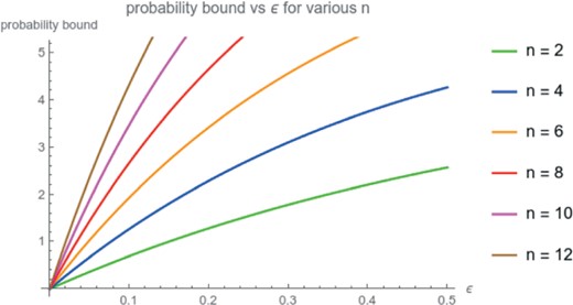
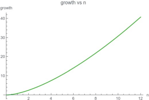
We defined a measure of |$\varepsilon $| uncontrollability in a Gaussian random ensemble of linear systems. We calculated tight bounds for this probability in terms of |$\varepsilon $| and the number of states |$n$|. This is also depicted in the graphs included in the appendix (Figs 1and 2).
Acknowledgements
The authors want to express their thanks to Professor D. Cheliotis for his valuable suggestions concerning random matrices. The authors are also indebted to the anonymous referees for their remarks, which improved the presentation of the results.
References
Anderson
, G. W.
, Guionnet
, A.
& Zeitouni
, O.
(
2010
)
An Introduction to Random Matrices
.
Cambridge Studies in Advance Mathematics
, vol. 118.
Cambridge
:
Cambridge University Press
.
Ball
, K.
(
1997
)
An elementary introduction to modern convex geometry
.
Flavors of Geometry
, vol. 31,
Cambridge
:
Cambridge Univ. Press
.
MSRI Publications
.
Folland
, G.
(
1999
)
Real Analysis: Modern Techniques and Their Applications
, 2nd edn.
Pure and Applied Mathematics
.
New York
:
John Wiley
.
Karkanias
, N.
& Milonidis
, E.
(
2007
)
Structural methods for linear systems: an introduction
.
Mathematical Methods for Robust and Nonlinear Control
.
Lecture Notes in Control and Information Sciences
, vol. 367.
Berlin
:
Springer
, pp.
47
–
98
.
O’Rourke
, S.
& Touri
, B.
(
2015
)
Controllability of random systems: universality and minimal controllability
. .
Polderman
, J. W.
& Willems
, J. C.
(
1998
)
Introduction to Mathematical Systems Theory: A Behavioral Approach
.
Texts in Applied Mathematics
, vol. 26.
New York
:
Springer
.
Appendix
In this appendix, we present
the diagram of the upper bound for |$\varepsilon $|-uncontrollability given in Theorem 5.2 (Fig. 1);
the diagram of the upper bound for the derivative |$\left . \frac{dP_{\varepsilon }}{d\varepsilon } \right |_{\varepsilon =0}$| given in Corollary 5.3 (Fig. 2).

Fig. 1.
The diagram of the upper bound of the |$\varepsilon $|-uncontrollability |$P_{\varepsilon }$| for several values of the number |$n$| of states.

Fig. 2.
The diagram of the upper bound for the growth rate of |$P_{\varepsilon }$| at zero.
© The Author(s) 2021. Published by Oxford University Press on behalf of the Institute of Mathematics and its Applications. All rights reserved.
This is an Open Access article distributed under the terms of the Creative Commons Attribution License (
https://creativecommons.org/licenses/by/4.0/), which permits unrestricted reuse, distribution, and reproduction in any medium, provided the original work is properly cited.
PDF


