Abstract
We study an elastic particle translating axially along the centre-line of a rigid cylindrical tube filled with a Newtonian viscous fluid. The flow is pressure-driven and an axial body force is applied to the particle. We consider the regime in which the ratio of typical viscous fluid stress to elastic stiffness is small, leading to small elastic strains in the particle. In this case, there is a one-way decoupling of the fluid–structure interaction problem. The leading-order fluid problem is shown to be pressure-driven Stokes flow past a rigid sphere, and is solved using the semi-analytical method of reflections. The traction exerted by the fluid on the particle can be computed and used to formulate a pure solid-mechanics problem for the deformation of the particle, which can be solved analytically. This framework is used to investigate the role of the background flow, an axial body force and the tube wall on the particle’s leading-order translational velocity, resulting deformation and induced solid stress. By considering the first-order fluid problem the next-order correction to the translational velocity of the particle is shown to be zero. Depending on the magnitude of the ratio of applied body force to viscous forces, the particle can either have a bullet-like shape, an anti-bullet shape, or retain its original spherical shape. A non-linear arbitrary Lagrangian-Eulerian finite element implementation is used, in conjunction with various existing results from the literature, to validate the method of reflections solutions and interrogate their range of validity.
1. Introduction
The motion of elastic bodies in low Reynolds number flows finds motivation in both industrial and scientific fields, with examples including the study of micro-gel beads, suspended polymer molecules and biological flows (Guido & Shaqfeh, 2019; Villone & Maffettone, 2019). In these examples, the fluid stress induces a deformation in the elastic solid which in turn alters the domain for the fluid, thus creating a non-trivial coupling between the fluid and solid phases (Geislinger & Franke, 2014; Barthès-Biesel, 2016; Nasouri et al., 2017; Villone & Maffettone, 2019). Predicting the internal stress experienced by a particle in a cylindrical tube is of particular interest when considering mechanosensitive particles. These include stiffer cells such as white blood cells and osteoblasts for which an elastic particle can form a simplistic model (Darling et al. 2008; Barakat et al. 2019). Upon exposure to mechanical stimuli, the intracellular cytoskeleton transfers stress to the cell nuclei, reproducibly upregulating expression of certain genes (Zhang et al., 2012; Li et al., 2019). Depending on the gene, a change in expression may directly correspond to a change in the cell’s properties (Jin et al., 2020). Modern experimental techniques motivate the study of biological cells exposed to a body force. Yeo et al. (2021) investigated how magnetically tagged cells are transported when exposed to a magnetic field, and Zhang et al. (2010) developed a method for dragging an individual cell in hydrodynamic flows using optical tweezers, which does not require direct contact with the cell itself. Further motivation comes from the use of hydrogel particles for drug delivery systems (Li & Mooney 2016). By injecting a solution containing drug-carrying hydrogel particles into the body, drug payloads can be delivered to specific sites in a minimally invasive procedure. However, the pressure-driven flow during injection can generate large shear stresses that damage the hydrogels and cause the premature release of drug molecules.
Much of the mathematical literature surrounding the motion of particles in low Reynolds number flows within a cylindrical tube is concerned with rigid bodies, with studies focusing on the effect of particle size, shape and initial position on its axial and lateral velocity (Brenner & Happel, 1958; Haberman, 1958; Greenstein & Happel, 1968; Bungay & Brenner, 1973; Leichtberg et al., 1976; Bhattacharya et al., 2010; Yeh & Keh, 2013). Relevant to our work, Yao & Marcos and Wong (2017) used the method of reflections (MoR), a semi-analytical, meshless method first developed by Brenner & Happel (1958), to calculate the velocity field around two rigid spheres arbitrarily positioned in a cylindrical tube, deriving a relationship between the rigid particle velocity and Stokes drag. The result forms an extension to Faxen’s law, which describes the relationship between particle velocity and Stokes drag for a single rigid sphere in an unbounded Stokes flow.
To our knowledge, there have been few analytical studies on the deformation of an elastic particle coupled to a viscous flow. Murata (1980) first touched the subject, asymptotically modelling the sedimentation of an elastic sphere in an unbounded, stationary fluid in the limit of a small ratio of viscous forces to solid forces, showing the particle undergoes no shape change to leading order. Nasouri et al. (2017) extended this framework to study the sedimentation of a two-sphere swimmer consisting of one rigid particle and one neo-Hookean particle in an unbounded, stationary fluid. Murata (1981) modelled an elastic particle in a general unbounded flow, with a key example being Poiseuille flow. This method combines the background Poiseuille flow with an additional velocity term of the fluid flow that ensures the boundary conditions on the particle surface are satisfied. Importantly, the method does not fully consider the effect of a tube wall on the deformation. Mietke et al., (2015) utilised the MoR to properly account for the tube wall in the leading-order fluid problem, obtaining semi-analytical results for the small deformation of a particle in equilibrium which translates on the centre-line of a rigid cylindrical tube. By imaging the steady deformation of a single cell travelling through a microfluidic square channel, this model was used to predict the Young's modulus of the cell. Later, Mokbel et al., (2017) used a numerical method to model the finite deformation of the elastic particle, predicting the Young's modulus of the cell using both a linearly elastic and neo-Hookean constitutive model. Villone & Maffettone (2019) used an arbitrary Lagrangian-Eulerian (ALE) finite element method (FEM) to characterise the mobility and deformation of an incompressible, neo-Hookean particle, modelled as a drop of an upper-convected Maxwell viscoelastic fluid with infinite relaxation time, in different Newtonian and non-Newtonian flows. Within a cylindrical tube, Villone et al. (2016) numerically calculated the lateral migration velocity of the particle for varying relative sizes and initial positions. Notably, each of these studies omit the presence of a body force acting on the particle. Noichl & Schönecker (2022) performed experiments investigating how the deformability of an elastic particle affects its sedimentation velocity in a channel of square cross section, finding poor agreement with existing analytical results (Murata 1980). This further motivates the study of how geometric confinement impacts deformable particles in viscous flow.
We model an elastic particle translating along the axis of the cylindrical tube in the limit of small viscous fluid stress to elastic stiffness, leading to small elastic strains in the particle. This limit allows the calculation to be split into two parts. First, the leading-order fluid problem is solved for a rigid sphere and the solution is used to compute the viscous traction at the sphere interface. The second part is to find the deformation of an elastic sphere subject to these tractions. We adopt a similar approach to Mietke et al., (2015), and use the MoR to more accurately impose no-slip boundary conditions on the tube wall. The MoR has been previously utilised to calculate Poiseuille flow around a single rigid sphere (Wakiya, 1953; Happel & Byrne, 1957; Brenner & Happel, 1958; Haberman, 1958; Greenstein & Happel, 1968; Murata, 1981), with the main differences between publications being the convergence criteria used to truncate the infinite system of equations that arise after successive reflections of the flow from the spherical and cylindrical boundaries. While explicit solutions are presented in these works, their accuracy is restricted by only considering a small number of terms due to computational limitations. Consequently, we use the MoR to solve the leading-order fluid problem from scratch in order to obtain a solution to any required degree of accuracy.
Previous authors have shown that the lateral migration forces acting on a deformable particle may be decomposed into an elastic restoring effect and a wall-induced lift, both of which push the particle toward the centre-line of the tube, together with inertial lift which pushes the particle away from the centre-line (see Schaaf & Stark (2017) and references within). Motivated by this, since we neglect fluid inertia, we assume the particle translates along the centre-line of the tube. We investigate steady flows and examine the individual effects of the background Poiseuille flow, axial body force and the addition of the tube wall on the translational velocity of the particle, the resulting deformation and the induced solid stress within the particle. We additionally investigate the impact of the particle deformation on the surrounding fluid and show that the effect on the particle's translational velocity is weak. We use results from Murata (1981), Bungay & Brenner (1973) and Villone et al. (2016), along with our own non-linear ALE finite element simulations, to comprehensively assess the validity of the analytic results. The MoR solutions give deeper analytical insight than the ALE FEM solutions and provide a more practical tool for interrogating the effect of changing the background Poiseuille flow, axial body force and particle size. The ALE FEM solutions, however, solve the full non-linear problem and so may be used to the investigate finite deformations and to quantify the range of validity of the MoR solutions.
This paper is structured as follows: in Section 2, we formulate the problem, non-dimensionalising through physical arguments. We then perform an asymptotic expansion in the limit of a small ratio of typical viscous fluid stress to elastic stiffness in Section 3. In Section 4, we present the semi-analytic MoR to solve the leading-order fluid and solid problems, alongside our non-linear ALE finite element method. In Section 5 we first study the cases of a particle exposed to a background Poiseuille flow only, and under an axial body force only, comparing our MoR solutions with pre-existing results from the literature and our ALE FEM solutions. We then use the MoR implementation to investigate the combined effects of a background Poiseuille flow and axial body force on the flow field, particle deformation and induced stress. Finally, we provide a closing discussion in Section 6.
2. Problem formulation
We model an initially spherical elastic particle translating axially along the centre-line of a cylindrical tube driven by Poiseuille flow in the far field and under the influence of an axial body force. We define spherical and cylindrical coordinate systems and , with corresponding unit vectors and , respectively. We align the -axis with the central axis of the tube and choose both origins to coincide with the centre of the particle as shown in Fig. 1. We assume the problem is axisymmetric and has reached a steady equilibrium. The maximum magnitude of the background tube flow is in the lab frame and the undeformed particle and tube radii are given by and , respectively. In the lab frame, the translational velocity of the particle, , is unknown and will generally depend on the particle size and its material properties. We work in the frame of reference of the centre of mass of the particle such that we see sliding walls with velocity . The fluid and solid domains are denoted by and , respectively, with the interface between the two denoted by .
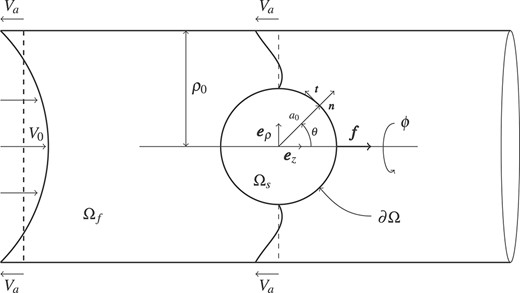
Fig. 1.
We consider an elastic particle translating with velocity along the centre-line of a cylindrical tube driven by Poiseuille flow in the far-field and subject to an axial body force . We work in the frame of reference of the translating particle, resulting in sliding walls of velocity . The fluid domain and solid domains are denoted by and , respectively, with the interface between the two phases denoted by .
2.1 Governing equations
The flow of fluid in the tube is governed by the incompressible Stokes equations,
where is the fluid velocity and is the stress tensor for a Newtonian viscous fluid given by
with the fluid pressure and the fluid viscosity. The superscript denotes the transpose. The above expressions are presented using Eulerian coordinates, and we formulate the solid problem also in Eulerian coordinates.
The elastic particle is governed by the conservation of momentum equation,
where is the solid stress tensor and is a constant body force acting on the particle in the axial direction. For the elastic constitutive relation, we choose an isotropic, incompressible neo-Hookean description,
where is the solid pressure, is the strain tensor and is the elastic shear modulus. The deformation gradient tensor, , is defined through its inverse , where is the displacement vector. The displacement vector is defined as , where is the position of a material point in the undeformed configuration and is the current position vector of this point. The incompressibility condition is imposed as
Under the assumption of infinitesimal strain, Equations (2.5) and (2.6) reduce to the equations of incompressible linear elasticity,
where is the linear elastic strain tensor. Equations (2.7), (2.8) are useful for informing the non-dimensionalsation and will guide our choice of perturbation parameter in Section 3.
We now present the boundary and interfacial conditions. Far upstream and downstream of the particle we impose Poiseuille flow of maximum magnitude in the lab frame in a tube whose walls have axial velocity ,
On the tube wall, , we impose
corresponding to no penetration and no-slip. Since we work in the frame of reference of the particle the no-slip and no-penetration boundary conditions on are given by
We impose continuinty of stress on ,
where is the outward-pointing unit normal to the surface of the deformed particle.
The deformation of the interface is denoted by
where is the position of the interface.
By integrating the stress balance (2.4), applying the divergence theorem and using the interfacial condition (2.12), we obtain the equilibrium relation,
where is the viscous drag exerted by the fluid on the elastic particle in the axial direction. This will be useful later for predicting the translational velocity of the elastic particle given a body force of magnitude .
2.2 Non-dimensionalisation
We non-dimensionalise as follows, using stars to denote dimensionless variables,
We non-dimensionalise lengths with the tube radius , velocities with , and fluid pressure and stress with the viscous pressure scaling. Motivated by the interfacial stress condition (2.12), we non-dimensionalise the solid pressure and stress identically to the fluid stress, and scale the axial body force appropriately to the momentum equation for the solid phase (2.4),
We introduce the parameter to characterise the size of the elastic strain, which is determined by dividing the solid stress by the shear modulus in (2.7). Having determined a scale for the elastic strain, it follows from the strain tensor that the solid displacement is of order , and is non-dimensionalised as
We henceforth drop the stars for convenience.
The full dimensionless problem is then governed by
in , and
in , where
In the limit of small we have the following:
The expansions (2.25) and (2.25) will be useful for the asymptotic analysis in Section 3.
The dimensionless boundary conditions in the far field are
and on the walls of the cylindrical tube, ,
On the fluid-particle interface, , we have
In addition to , we have two further dimensionless values: , the blockage factor, which is the ratio between the undeformed particle and tube radii, and , which represents the ratio between the translational velocity of the particle and the maximum magnitude of the Poiseuille flow in the lab frame. The equilibrium condition (2.14), used to calculate the particle’s translational velocity, remains the same after non-dimensionalisation.
3. Asymptotic analysis of a stiff particle
We now assume that , corresponding to the limit of a stiff particle, and expand variables in powers of ,
where the superscript denotes the associated power of . We similarly expand the translational velocity of the elastic particle, the viscous drag and the position of the interface,
We proceed by assuming , and the body force magnitude , are as . At each order in , we separate the problem into the respective fluid and solid parts. We show that the leading-order fluid problem decouples from the solid problem and is therefore not impacted by the deformation of the particle. The fluid stress provides a surface traction on the elastic particle that drives the leading-order solid problem.
In the analysis that follows, we impose a body force , and calculate the translational velocity . We could equally solve the inverse problem using this framework by fixing the translational velocity and calculating the body force required to achieve this translational velocity equilibrium through (2.14). In this case we would asymptotically expand the body force , as the translational velocity is prescribed.
3.1 Limiting geometries
While not the focus of the present study, it is important to comment on the case when . Previously in Section 3, we characterised the solid strain by the dimensionless parameter , requiring to satisfy the small strain assumption. However, assuming the tube remains rigid, we expect the pressure in the lubrication layer between the tube wall and particle to increase such that assumption of infinitesimal strain is broken, even for . This suggests a restriction on related to the particle size . Bungay & Brenner (1973) studied a tightly-fitting, concentrically positioned rigid sphere in a cylindrical tube, finding that, for the cases of pressure-driven flow around a stationary particle and a particle translating through an otherwise stationary fluid, the fluid pressure in the lubrication region scales with to leading order in , where . It was also shown that the shear stress in the lubrication region scales with such that the pressure forms the main contribution to the stresses acting on the particle. Thus, by using the pressure scale in the lubrication region as a measure of the fluid stress exerted on the particle and imposing stress conservation across the boundary, it follows that for , in order for the solid strain in the particle to be small, we require
Assuming is small, we may also rearrange (3.4) to predict the range of suitable particle sizes for fixed ,
We expect similar restrictions to apply with a general combination of pressure-driven flow and axial body force but these require a detailed asymptotic analysis that is beyond the scope of this paper.
We can also consider the case . In this case, the spatial variables for the solid problem must be rescaled according to , in which case the stress tensor becomes
Consequently, for small we require
to satisfy the infinitesimal strain assumption, suggesting the asymptotic expansion in remains valid for a wider range of for compared with .
3.2 Leading-order fluid problem
The leading-order incompressible Stokes equations are
Expanding the kinematic condition (2.30) we find , implying boundary conditions are applied on the undeformed particle surface, a sphere of radius . The boundary conditions (2.26)–(2.27) at leading order give
Equations (3.8–3.12) form a full description of the leading-order fluid problem. The particle does not deform at this order and so the leading-order fluid problem is equivalent to a rigid sphere under axisymmetric, pressure-driven tube flow subject to an axial body force. We note that the leading-order fluid pressure is determined up to an arbitrary constant and we choose to set at and . To leading order, the equilibrium condition (2.14) gives
where the leading-order magnitude of the Stokes drag acting on the particle is given by
Noting that depends linearly on the magnitude of the background Poiseuille flow and particle velocity, so too do and . We can thus write a dimensionless, revised version of Faxen’s law as
defining and as the wall correction factors (Yao et al., 2019). Substituting the expression for (3.15) into Equation (3.13) we obtain the explicit result for the leading-order translation velocity,
Setting in Equation (3.16) we obtain the leading-order translational velocity under no applied body force, motivating the decomposition
By decomposing the translational velocity in this way, we split the leading-order fluid problem into two parts: a rigid sphere under no body force driven by Poiseuille flow in the tube, resulting in the translational velocity , and a rigid sphere subject to an axial body force with no background flow, resulting in the translational velocity . The explicit dependence on body force given by is similar to that obtained by Murata (1980) for an elastic particle under a body force in an unbounded domain, with the addition of capturing the effect of the tube wall.
3.3 Leading-order solid problem
The leading-order equilibrium equation for the solid is
where combining (2.25) and (2.22), we reduce to a linearly elastic stress–strain relationship to leading order
The incompressibility condition is then given by Equation (2.25)
such that the leading-order solid displacement and pressure are also governed by Stokes equations. The interfacial condition (2.29) gives
and the kinematic condition (2.30) at leading-order gives
3.4 First-order fluid problem
We consider the first-order correction to the flow field around the elastic particle. We again have the Stokes equations relating fluid velocity and pressure at this order, Equations (3.8) and (3.9). The far-field condition (2.26) gives
where captures how the leading-order deformation of the particle affects its translational velocity within the tube. The velocity condition on the tube wall is
while the velocity condition (2.28) at gives
where we have used the fact that
Expanding Equation (2.14), the viscous drag acting on the particle at first order is
where denotes the cross product and we have expanded the magnitude of the surface deformation as
We show later in Section 4.1.4 that the first-order correction to the translational velocity .
4. Solution methods
4.1 Semi-analytical implementation
Solving the leading-order fluid problem involves a mix of geometries; the cylindrical tube motivates the use of a cylindrical coordinate system, while the undeformed particle is more naturally considered via a spherical coordinate system. To account for this mix of geometries, we choose to employ the MoR, though we could equally select another suitable method, for example a collocation technique or boundary element method (Wen et al., 2007; Saad & Faltas, 2014).
In this subsection we introduce the MoR and apply it to the leading-order fluid problem. We then consider the leading-order solid problem, presenting general solutions for the deformation and relevant stress components. Finally, we consider the first-order fluid problem, showing the first-order correction to the translational velocity is zero.
4.1.1 Method of reflections
The method of reflections, originally developed by Brenner & Happel (1958), is a meshless semi-analytic method which involves splitting up the problem such that only one set of boundary conditions, and consequently coordinate system, are considered at any time. We present full details of the MoR in Appendix A and direct the interested reader to Yao & Marcos and Wong (2017); Yao et al. (2019) for further information. Due to the linearity of the Stokes equations and boundary conditions we can decompose the velocity field as follows:
where corresponds to the -th term in the series for , and are the terms in the asymptotic expansion; see Section 3. Terms with odd (, ) are calculated by solving Stokes equations using a spherical coordinate system and imposing the interfacial conditions on the particle, while terms with even (, ) are calculated by solving Stokes equations using a cylindrical coordinate system and imposing the boundary conditions on the tube wall. Since each term corresponds to a reflection, the addition of a new term using either a spherical or cylindrical coordinate system, is defined as the reflection number.
4.1.2 Leading-order fluid problem
We apply the MoR to solve the system of equations defining the leading-order fluid problem (3.8)–(3.12). We begin by choosing
which ensures all other velocity components must vanish for , or equivalently for contributions in spherical coordinates, . Equation (4.2) guarantees we satisfy the far-field condition (3.10) and the boundary conditions on the tube wall (3.12). The only conditions left to satisfy are the boundary conditions on the surface of the sphere (3.11). To address this, we transform to spherical coordinates (details given in Appendix A.1) and introduce such that together satisfy the boundary conditions on the surface of the sphere. By including the velocity component we disrupt the boundary conditions on the tube wall, (3.12). To reimpose these boundary conditions, we convert the expression to cylindrical coordinates, and add such that satisfies Equation (3.12). This process repeats indefinitely with calculated by satisfying Equation (3.12) using a cylindrical coordinate system, and found by satisfying Equation (3.11) using a spherical coordinate system. We summarise the process via the following equations:
If we truncate the velocity series at an odd term then we fully satisfy the interfacial condition on the surface of the sphere, with an error on the tube wall. If we truncate the velocity series at an even term then the opposite is true. We define a solution as having converged when the most recent contribution to the net force acting on the sphere is at least five orders of magnitude smaller than the net force from all components. The details of this are presented in Appendix A.4.
The final solution obtained involves a combination of expressions in both spherical and cylindrical coordinate systems, which each individually satisfy Stokes equations, and when added satisfy both the boundary conditions on the tube wall and boundary conditions on the sphere surface simultaneously. Crucially, we can obtain semi-analytical expressions for the fluid velocity, pressure and stress on the undeformed boundary of the sphere at . The semi-analytic nature of these expressions originates from the integrals present in the general solution for the velocity field in cylindrical coordinates (A.17)–(A.19) which must be evaluated numerically. Consequently, the expressions for the total velocity field in spherical coordinates are of the form
where are the Legendre polynomials of order and are the Gegenbauer polynomials of order and degree . The subscripts and correspond to the radial and azimuthal components of a vector in spherical coordinates, respectively, and the subscript corresponds to the summation. We write the associated pressure field as
and the relevant stress components using the fluid constitutive relation (2.20),
Here, the tensor components, . In Equations (4.7–4.11) the coefficients and arise naturally from the stream function series for the velocity field in spherical coordinates, see (A.4), while the coefficients arise from projecting terms calculated using a cylindrical coordinate system onto the undeformed particle surface via Equations (A.9) and (A.10). All of these projections are performed numerically due to the difficulty of converting the general solutions for velocity and stress from cylindrical to spherical coordinates. To solve the leading-order fluid and solid problems, we use the first three non-zero terms in the stream function series that correspond to . This is because the far-field flow can be written exactly using terms with and and, under this external flow, the presence of the tube wall exclusively drives terms with even in the stream function series. The impacts of this truncation choice on solution accuracy are discussed in Appendix A.4.
The fluid normal and shear stress calculated from the leading-order fluid problem act as tractions to drive a deformation of the elastic particle. From the MoR we have known, semi-analytic expressions for these forcing terms given by Equations (4.10) and (4.11).
4.1.3 Leading-order solid problem
At this order the solid displacement is governed by Stokes equations with a body force. Restricting to terms that remain finite as , the solution is given by Happel & Brenner (1991)
We calculate the relevant stress components using the constitutive relation (3.19),
In general, and in Equations (4.15) and (4.16) are calculated by imposing continuity of traction on the particle surface (3.21). We then obtain the solid displacement by substituting and into Equations (4.12) and (4.13), with the position of the free surface given by Equation (3.22). The coefficient in Equation (4.12) corresponds to translation and so does not generate any stress in Equations (4.15) and (4.16). Since is not set by the interfacial conditions we must impose another condition to pin this degree of freedom, choosing to set the net axial displacement to be zero by considering
Substituting the above expressions for displacement (4.12) and (4.13) into (4.17) gives
such that the centre of mass of the particle is unchanged when deformed.
4.1.4 First-order correction to the translational velocity
We again apply the MoR to solve the first-order correction to the local flow field outlined by Equations (3.23–3.25). Since the leading-order fluid and solid problems involve only terms with even (see Section 4.1.2), we see the velocity condition on the particle surface (3.25) generates terms with odd in since and contain only terms with even . Terms with even arise due to the unknown first-order correction to the translational velocity, generated by the far-field condition (3.23) and the boundary conditions on the tube wall (3.24) since even terms satisfy the wall conditions. Critically, in Equation (27) terms with odd do not contribute to the net drag on the particle and so we find that
such that the first-order correction to the translational velocity is zero. We interpret this result via a consideration of symmetry. We expect the velocity of a deformable particle to be an odd function of the applied body force and pressure gradient across the tube as inverting the direction of either changes the sign of the particle velocity. The leading-order velocity depends linearly on the applied body force and pressure drop and is the same for both a deformable particle and a rigid sphere of the same radius. The first-order contribution to the particle velocity is forced by (3.25) and so is quadratic (even) in both the applied body force and pressure drop. It is therefore necessary to calculate the second-order contribution to the particle velocity expansion to see a difference between rigid and deformable particles.
We note that the second-order contribution to the particle velocity could, in theory, be obtained through the use of the reciprocal theorem, which would avoid the explicit calculation of the full second-order velocity field (Masoud & Stone 2019). This method relies on the construction of integral relations through the reciprocal theorem, which are simplified through knowledge of the boundary conditions on the second-order velocity field. The use of the reciprocal theorem to predict the second-order contribution to the particle velocity would require the calculation of the first-order particle deformation and is beyond the scope of the present study. Here, we instead utilise fully non-linear finite-element simulations to investigate higher-order contributions to the particle velocity and other quantities of interest.
4.2 Finite element implementation
To investigate the range of validity of the MoR solutions, we solve the full non-linear fluid–structure interaction (FSI) problem via the finite element method using an ALE approach. We construct a steady, 2D axisymmetric implementation which greatly improves efficiency (typically minute per simulation) compared to the previous time-dependent, 3D numerical study by Villone et al. (2016), which took an average of 2–3 days per simulation. For convenience, we instead work in the lab frame such that the particle translates with velocity . For brevity, we present a brief overview of the method here, with details of the ALE problem formulation and its validation presented in Appendix B. The ALE approach couples the Lagrangian solid problem with the Eulerian fluid problem, which is transformed into a Lagrangian frame via the fluid mesh displacement such that the undeformed reference configuration is used as the computational domain. The fluid mesh displacement has no physical interpretation, and acts to project the solid displacement into the fluid domain. Consequently, an arbitrary governing equation may be used to calculate the fluid mesh displacement; in this study, we use the equations of linear elasticity for the fluid mesh displacement.
We use the finite element library with the additional package to implement the ALE method, generating meshes via gmsh (Logg et al., 2012; Alnaes et al., 2015; Ballarin, 2022; Geuzaine & Remacle, 2022). We use elements for the fluid velocity, solid displacement and fluid mesh displacement and use elements for the pressures. Moreover, we employ Lagrange multipliers to impose zero mean displacement of the particle (4.17), a zero mean fluid pressure to pin the arbitrary reference pressure which is identical to the MoR reference pressure condition to leading order, to account for the stress balance on the particle surface (2.29), to impose the force balance (2.14) and calculate the equilibrium particle velocity, to ensure the continuity of fluid and solid velocity on the particle surface, and to impose the continuity of the solid and fluid mesh displacements on the undeformed particle boundary. Natural-parameter continuation was used to compute solutions across a range of values of .
5. Results
We now present results from both the MoR solutions and the non-linear ALE FEM solutions. We begin by considering the case of a particle in Poiseuille flow with , discussing the particle velocity and deformation. We then provide similar results for the case of a particle translating under an axial body force with no background Poiseuille flow. We use the ALE FEM solutions, along with relevant results from the literature where possible, to both validate the MoR solutions and probe their range of validity. Finally, we use the MoR implementation to investigate the combined impacts of the Poiseuille flow and body force on the particle shape, experienced stress and the surrounding velocity field.
5.1 A particle in Poiseuille flow
We first present the wall corrections factors for the leading-order fluid problem in Fig. 2, obtained by substituting the fluid stress into Equation (3.14) and isolating the parts which depend on the background Poiseuille flow and the particle velocity. We also present the equivalent results by Bungay & Brenner (1973), obtained using a lubrication approximation for a rigid particle as .
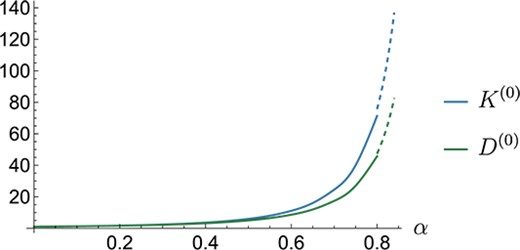
Fig. 2.
Wall correction factors, and , for varying . The solid lines are our MoR solutions and the dashed lines are adapted from Bungay & Brenner (1973), and were obtained using a lubrication approximation with a rigid particle.
Under no axial body force, the leading-order translational velocities. are given by the ratio of and in Fig. 2. We plot these MoR velocities against our FEM predictions for varying in Fig. 3(a), using three different values of for the FEM predictions. We additionally plot the results by Murata (1981) and Bungay & Brenner (1973) which are valid for small and tightly-fitting rigid particles, respectively. The purely analytical solution by Bungay & Brenner (1973), obtained in the limit , diverges quickly from the MoR and FEM solutions such that we observe a discrepancy from the FEM solution even for . Conversely, the purely analytical solution by Murata (1981) provides a good approximation for small , but diverges as increases. This too is expected, as Murata does not fully consider the tube wall, instead assuming the Poiseuille flow is unbounded. Murata’s solution is identical to that obtained by the method of reflections with reflection number . If the particle size is small compared to the cross section of the tube then the influence of the tube wall on the flow, and thus its impact on the stresses at the particle’s surface, which results in the translation of the particle, is small. Both our MoR and FEM approaches impose no-slip on the tube wall, allowing the effect of the tube wall on the particle to be captured fully. This is ensured for the method of reflections if sufficient reflections are included for convergence and in the spherical stream function series is large enough to accurately project cylindrical contributions to the undeformed surface of the particle when calculating and in Equations (4.7–4.11). Our MoR solutions are presented for since the number of reflections required for a solution increases with and the choice of three non-zero terms in the spherical stream function series, corresponding to , is not enough for accurate projection when . Both issues are discussed and quantified in Appendix A.4.
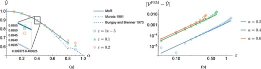
Fig. 3.
(a) Predicted velocity of a particle under a background Poiseuille flow () for varying . Graphs are shown for the MoR (solid lines) and our finite element implementation for different (squares, triangles and circles), as well as for the implementations by Murata (1981) and Bungay & Brenner (1973) which are valid for small and tightly-fitting rigid particles, respectively. (b) Log-log plots of the norm of the absolute error between the non-linear FEM solution and the MoR solutions, increasing for three different particle sizes. In each case, the non-linear particle velocity is smaller than the MoR prediction (see, for example, the inset in (a)). Linear lines of best fit are also presented, omitting the clear non-linear trend for . The average slope across the three lines is .
We observe strong agreement between our MoR and FEM solutions when is small, validating the method of reflections for this application. As increases the non-linear predictions begin to diverge from the MoR predictions. In Fig. 3(b), we quantify this divergence for three different particle sizes, presenting log-log plots of the norm of the absolute error between the FEM and MoR particle velocities over a wide range of . In each of these plots, we increase until the FEM implementation no longer converges, and note that the non-linear FEM predictions are in fact smaller than the MoR predictions. In each plot we observe a roughly straight line with average slope , indicating the predicted quadratic departure of the non-linear solution. We note that the data points with and are due to the accuracy limitations associated with the truncation choices in the MoR, and the numerical nature of the FEM solution which are larger than the perturbation error. In general, we observe that the error increases with particle size for fixed as expected from (3.4) and (3.7), and note that with a smaller particle larger values of were attained before the FEM solver failed to converge. We acknowledge that the range of tested in Fig. 3(b) is large, with reaching when , but stress that despite this, the MoR solutions can predict the non-linear particle velocity to within for all tested combinations of and .
Interestingly, the sign of the discrepancy between the our MoR and FEM solutions is dependent on the particle size; though slight, the particle velocity decreases with when in Fig. 3(a) and increases with as (see in Fig. 3(a)). For an elastic particle sedimenting in an unbounded flow, Nasouri et al. (2017) showed that an incompressible particle’s terminal velocity is slightly decreased () when compared with a rigid particle. This dependency is similarly observed here for particles with under tube confinement. We expect this is a result of the axial compression causing bulging of the particle out toward the tube wall (see Fig. 4), increasing the particle’s drag. For larger particles, however, we observe the reverse dependence. Here, we expect the particle deformation to involve an axial elongation, increasing the width of the lubrication layer between the particle and tube wall and resulting in an increased particle velocity. This is analogous to the results of Barakat & Shaqfeh (2018), who studied the motion of closely fitting vesicles under cylindrical confinement with varying initial shapes including spherical.
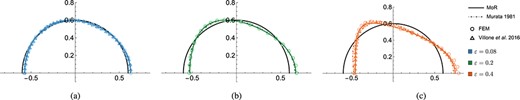
Fig. 4.
Surface deformation with and for (a) , (b) and (c) . Graphs are shown for both the MoR (solid, coloured lines) and our ALE FEM implementation (circles), as well as for the implementations by Murata (1981) and where possible Villone et al. (2016). In each plot, we also show the undeformed particle boundary via the solid, black lines (colour online).
We now calculate the leading-order surface deformation of the particle, presenting results in Fig. 4. Here, we compare our MoR and FEM solutions for various values of with the implementation by Murata (1981), and, where possible, the ALE FEM fluid structure interaction simulations conducted by Villone et al. (2016). For small (Fig. 4(a)), we see agreement between all four methods. As we increase , the analytical predictions begin to diverge from the non-linear FEM solutions. Murata (1981) is the first to diverge due to the lack of proper consideration of the tube wall. With the tube wall properly considered, our MoR solutions more accurately mimic those predicted by both our FEM solutions and those by Villone et al. (2016), achieving the predicted bullet-like shape at .
We quantify the performance of the MoR solution in comparison to Murata (1981) in Fig. 5, where we present log-log plots of the -norm of the departure of the FEM displacement from the MoR solutions and those predicted by Murata (1981), averaging across the particle boundary. For each tested we observe a comparatively smaller error in the MoR deformation, as was qualitatively observed in Fig. 4. The slope of each line of best fit reflects the dependence of the departure on . As expected, the MoR plots have an average slope of , since the MoR solutions accurately approximate the contribution to the particle deformation. Instead testing the Murata (1981) predictions, we observe an average slope of , indicating the purely analytic solution does not predict the leading-order particle deformation as accurately as the MoR solution.
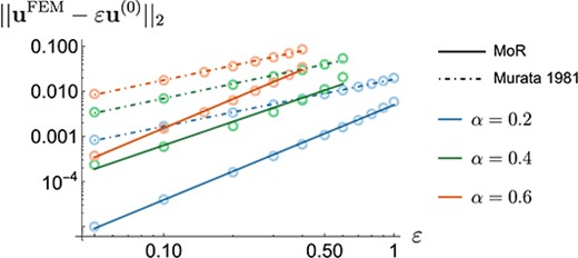
Fig. 5.
Log-log plots of the -norm of the departure of the FEM displacement along the particle boundary from the MoR solutions (solid lines of best fit) and Murata (1981) (dot-dashed lines of best fit) for three different values of . Here, the average gradient using the MoR solution is and using Murata is .
5.2 A particle under an axial body force
We now investigate the impact of applying an axial body force with magnitude with no driving Poiseuille flow. We note that if the body force here is the effect of gravity, we model the sedimentation of a particle under tube confinement. In Section 2.2, we non-dimensionalised using the Poiseuille velocity . In the absence of the background Poiseuille flow, the velocity scale is redefined and determined by balancing viscous stresses with the body force to obtain , where is the typical body force magnitude. Using this scaling, we recover Equation (3.17), which determines the relationship between the body force and particle velocity . In Fig. 6(a), we present for varying particle sizes, choosing the dimensionless to obtain an range which is comparable to the above analysis for a particle in Poiseuille flow. We present MoR and FEM predictions, and also the results of Murata (1980) and Bungay & Brenner (1973), which describe rigid particles sedimenting in an unbounded flow and under strong tube confinement, respectively. We note that the behaviour as , , is a consequence of the choice of length scale , which is convenient for the MoR. In this limit, the total body force applied to the particle is proportional to and the Stokes drag force is proportional to , resulting in the observed behaviour. Re-dimensionalising (3.17), we recover consistency with the standard result for the sedimentation velocity of a rigid particle in an unbounded flow. Conversely, as , is decreased by the tube wall, since in this limit. The trade-off between these two effects leads to a maximum translational velocity at an intermediate value when . At this value, we see the largest translational velocity for a given body force.
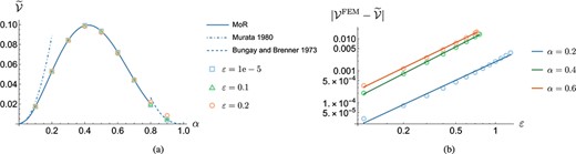
Fig. 6.
(a) Equilibrium velocity of a particle with and no background Poiseuille flow for varying . Graphs are shown for the MoR (solid lines) and our finite element implementation for different (squares, triangles and circles), as well as for the implementations by Murata (1980) and Bungay & Brenner (1973) which are valid for small and tightly-fitting rigid particles, respectively. (b) Log-log plots of the norm of the absolute error between the non-linear FEM solution from the MoR solutions, increasing for three different particle sizes. Linear lines of best fit are also presented with the average slope being .
We see Murata’s prediction, which considers an unbounded external flow, quickly diverges from the MoR solution for an equivalent particle under tube confinement. The prediction by Bungay & Brenner (1973) also diverges from the MoR and FEM predictions when . Unsurprisingly, the MoR and FEM predictions are consistent for small .
In Fig. 6(b), we present log-log plots of the norm of the absolute error between the FEM and MoR predictions for the particle velocity over a wide range of , similar to Fig. 3(b) for a particle in Poiseuille flow. We note the FEM predictions are smaller than the MoR solution for each presented and again observe quadratic divergence, with the average slope of . We observe the absolute error is comparable to Fig. 3(b), though we note the relative error is larger than in the purely pressure-driven case since the particle velocity in Fig. 6(a) is typically .
For an elastic particle subject to an axial body force in an unbounded domain the leading-order surface deformation is zero (Murata, 1980; Nasouri et al., 2017). Consequently, any leading-order surface deformation predicted by our MoR and finite element implementations is caused directly by the tube walls. In Fig. 7, we present surface deformation plots for varying , again choosing . For a positive , we observe a similar bullet-like shape to that induced by the Poiseuille flow, though note the particle appears to have a shorter axial length. We attribute the decrease in particle velocity in Fig. 6(a) to the bulging effect this has on the particle, most visible in Fig. 7 with in the FEM solution, decreasing the gap width between the particle and tube wall. As we expect instead that the particle is stretched along the -axis, resulting in an increased gap width Barakat & Shaqfeh (2018). This stretching increases the particle velocity as observed in Fig. 6(a) when . We also computed along the particle boundary, which again indicated the error of the MoR solution was .
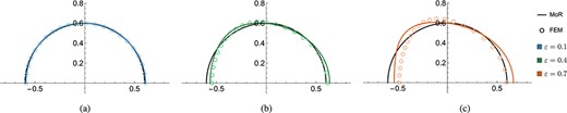
Fig. 7.
Surface deformation with , and no driving Poiseuille flow for (a) , (b) and (c) . Graphs are shown for both the MoR (solid, coloured lines) and our ALE FEM implementation (circles). In each plot, we also show the undeformed particle boundary via the solid, black lines (colour online).
5.3 Combined effects of the Poiseuille flow and body force
Having validated the MoR solutions using the non-linear ALE FEM implementation, we proceed by only considering the MoR solutions, and operating within their tested range of validity. We investigate the combined effects of the driving Poiseuille flow and applied body force by linearly combining the velocities, stresses and deformations obtained from separately solving the problems with no applied body force and no driving Poiseuille flow. For consistency, we again scale the velocity on the background Poiseuille flow by using as presented in (2.9). From these individual problems, we observe both left and right-pointing bullet-like shapes suggesting that for a given , there exists a negative (pointing upstream) body force magnitude such that these shapes approximately cancel. When this critical body force is applied, we see little surface deformation, though it is not identically zero. This critical body force at which we predict little surface deformation is represented in Fig. 8 by the green line, where we use the deformation at as a metric to represent this scenario. The surface displacement of the particle at is positive above the green line and negative below such that Fig. 8 forms a phase diagram, with the particle taking the shape of a rightward-pointing bullet above the green line, and a leftward-pointing bullet below it. Examples of these bullet-like shapes are inset in Fig. 8, with each one corresponding to the closest red dot.
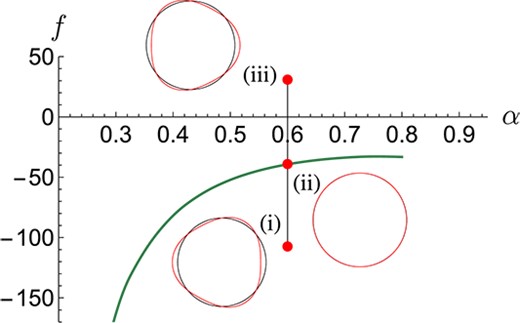
Fig. 8.
Deformation phase diagram for different and . The solid green curve corresponds to the critical velocity at which there is little deformation of the particle boundary (colour online). Above this line the shape is that of a bullet pointing to the right, and below the shape is that of a bullet to the left. Examples of the surface deformation are given with (undeformed particle in black), with each corresponding to the closest red dot. The applied body forces corresponding to the labels (i), (ii) and (iii) are and , respectively. Plots generated using our MoR implementation.
Within the context of mechanosensitive particles, it is important to consider how the solid stress, in particular the shear stress , is distributed throughout the bulk of the particle. Fig. 9 details the minimum and maximum values of with for a range of axial body forces; the range of stress values obtained throughout the bulk is contained in the shaded region. With , we have no body force and thus observe the stress developed purely due to the background Poiseuille flow. To study the induced stress in the bulk we consider three choices for the applied body force and from left to right, which correspond to the translational velocities and . As shown in Fig. 8, these choices, marked by the red dots, serve as examples for the different kinds of surface deformation: a leftward-pointing bullet, little radial deformation at and , and a rightward-pointing bullet. Within each particle plot the upper half is the MoR solution and the lower half is the numerical solution. With (), the particle is pinned in the lab frame and so is negative in the upper half, corresponding to clockwise shear, and positive in the lower half, corresponding to anti-clockwise shear. For the plots with little deformation at , corresponding to (), we see a similar profile, except with a lower magnitude since the sliding wall reduces the shearing effect of the background Poiseuille flow on the particle surface. With (), we see that the shearing effect from the sliding wall now dominates such that with and in the upper half is positive, corresponding to anti-clockwise shear. Closer to the tube axis, we still observe negative in the upper half, due to the shearing effect of the Poiseuille flow. By increasing the body force magnitude further, the sliding wall would dominate more strongly such that is completely positive in the upper half and negative in the lower half.

Fig. 9.
Maximal and minimal value of for varying translational velocities with , where the shaded region indicates the range of values obtained throughout the particle bulk. For ((i), (ii), (iii)), we present the stress throughout the bulk of the particle. These values are chosen identically to those in Fig. 8, and are representative of the different key boundary shapes obtained by the particle. Here, red and blue correspond to positive (anti-clockwise) and negative (clockwise) stresses, respectively (colour online). The stress has been calculated using the MoR.
This is evident in Fig. 10 where we present the corresponding leading-order and first-order streamline plots with the body force magnitudes and . In Fig. 10(a), when the particle is pinned in the lab frame, the streamlines divert around the sphere generating a large clockwise shear stress on the particle surface, concentrated around . In Fig. 10(b), at the critical force in which we observe little deformation (), the streamlines are more horizontal, resulting in a reduced shear stress on the particle surface. In Fig. 10(c), where the particle velocity , we observe a circulation region between the particle and the tube wall. Here, the body force instead forces the translational velocity of the particle to exceed the background Poiseuille flow. As a consequence of the tube wall the motion of the particle to the right forces fluid back upstream, resulting in the circulation region. The faster the particle, the more pronounced the circulation region. Consequently, the shear stress imposed on the sphere and the magnitude of the deformation are also larger. By manipulating the particle’s velocity using a body force the traction in the upper half of the particle varies from clockwise to anticlockwise shear and determines the left and right-bullet shapes observed in Figs 8 and 9.
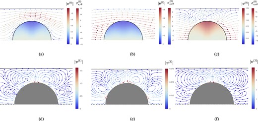
Fig. 10.
Leading-order ((a), (b), (c)) and first-order ((d), (e), (f)) streamline plots in the lab frame of reference with and . Plots generated using our MoR implementation. We present the corresponding in the leading-order plots throughout the undeformed particle bulk and note that here plots (a) and (b) correspond to (i) & (ii) as presented in Fig. 9. The latter case , corresponding to a particle velocity , is chosen to demonstrate the circulation region that is present when the particle is accelerated faster than the background Poiseuille flow.
We also consider the effect of the leading-order deformation on the flow field, presenting streamline plots for the first-order correction in Figs 10(d) to 10(f). Since the first-order contribution to the particle velocity is zero, the first-order correction to the flow field only accounts for the surface deformation of the particle through (3.25). The magnitude of the flow field is largest on the particle surface when where we observe the largest shear stress. The magnitude of the first-order correction decays quickly away from the particle surface to account for the remaining boundary conditions (3.23) and (3.24). We note that the magnitude of the first-order correction to the flow field is far smaller in Fig. 10(e) which reflects the small leading-order displacement observed in Fig. 8. The sign of the leading-order velocity field in the particle frame drives the direction of its resulting left-right bullet shape such that we observe similar circulation regions in each plot.
6. Conclusions
We present an asymptotic model for an elastic particle translating axially along the centre-line of a cylindrical tube, subject to an axial body force and driving Poiseuille flow. We work in the limit of a small ratio of viscous fluid stress to elastic stiffness and calculate the leading-order flow field, deformation and relevant stress components. We show that the leading-order fluid problem decouples from the leading-order solid problem and solve for the fluid flow around a rigid sphere. The leading-order fluid tractions are substituted into the leading-order solid problem to calculate the resulting deformation and solid stress components. We then consider the first-order fluid problem and find that the leading-order deformation does not affect the next-order translational velocity. This was known for an elastic particle in an unbounded flow and has been extended here to include tube confinement. This result has important implications for interpreting the experimental results of Noichl & Schönecker (2022) who observed large deviations in sedimentation velocity () for small, stiff, non-heavy particles () when compared with a rigid particle. One explanation for their observation of a large difference in velocity compared to our prediction of a small difference is that the experimental system does not reach steady state, which could be due to the effects of inertia in the fluid or the finite axial length of the domain. We also present a non-linear numerical finite element model used to validate the MoR solutions and investigate their range of validity. We find that the leading-order MoR solutions form an accurate simplification of the non-linear problem over a considerable range in and , especially for the case of a particle in Poiseuille flow. Moreover, we quantify the quadratic departure between the two solution methods for the predicted particle velocity and surface displacement. Where possible, we also compare our solutions to those in the literature, finding the MoR provides semi-analytic solutions that hold across a range of where previous analytical solutions do not apply.
The above results could be exploited in physical systems. For example, a body force could be selected in order to minimize deformation and preserve the initial spherical shape of a particle. A body force could equally be chosen to minimise the shearing effect on the particle or pin the particle in the flow. A better understanding of the mechanical response of an elastic particle in a flow is relevant to the study of biological cells and the development of drug delivery systems. Due to the simplicity of the problem geometry the predicted surface deformation could be experimentally validated for either a sedimenting sphere in a quiescent fluid, a sphere in equilibrium with Poiseuille flow Mietke et al., (2015), or a combination of both. The translational velocities of rigid and deformable spheres could also be compared to verify the weak impact of surface deformation on translational velocity. Once validated experimentally, one could use these results as a tool for the characterisation of the elastic properties of the particle as has been done with previous studies (Mietke et al., 2015; Mokbel et al., 2017; Villone et al., 2019). If a greater precision is required, the MoR could again be used to solve the first-order solid problem. This could then be used in conjunction with the reciprocal theorem, or through calculation of the second-order fluid problem, to better understand the impact of elasticity on the particle velocity. Murata (1980) showed that a compressible particle in an unbounded flow may have an increased or decreased velocity depending on its elastic constants. The effects of compressibility could also be investigated using our framework. More generally, this framework is applicable to systems with more complex physics. Assuming an initially spherical shape, one could model a poroelastic particle, include a poroelastic coating, or predict the flow around two deformable particles as in Yao & Marcos and Wong (2017).
Acknowledgments
The authors thank professor Ricardo Ruiz Baier for help with FEniCS and multiphenics.
Funding
Engineering and Physical Sciences Research Council studentship (EP/V520202/1 to S.M.F.); MRC (MR/T015489/1 to S.L.W.).
For the purpose of Open Access, the author has applied a CC BY public copyright licence to any Author Accepted Manuscript (AAM) version arising from this submission.
Conflicts of interest
The authors declare no conflicts of interest.
Code availability
Our ALE FEM implementation is freely available at the GitHub repository: https://github.com/finneysimon/stokes_elasticity_ALE_FSI.git.
References
Alnaes
,
M. S.
,
Blechta
, J.
,
Hake
, J.
,
Johansson
, A.
,
Kehlet
, B.
,
Logg
, A.
,
Richardson
, C.
,
Ring
, J.
,
Rognes
, M. E.
&
Wells
, G. N.
(
2015
)
The FEniCS project version 1.5
.
Arch. Numer. Soft.
,
3
.
Ballarin
,
F.
(
2022
)
Multiphenics – easy prototyping of multiphysics problems in fenics
. .
Barakat
,
J. M.
&
Shaqfeh
, E. S. G.
(
2018
)
Stokes flow of vesicles in a circular tube
.
J. Fluid Mech.
,
851
,
606
–
635
.
Barakat
,
J. M.
,
Ahmmed
, S. M.
,
Vanapalli
, S. A.
&
Shaqfeh
, E. S. G.
(
2019
)
Pressure-driven flow of a vesicle through a square microchannel
.
J. Fluid Mech.
,
861
,
447
–
483
.
Barthès-Biesel
,
D.
(
2016
)
Motion and deformation of elastic capsules and vesicles in flow
.
Annu. Rev. Fluid Mech.
,
48
,
25
–
52
.
Bhattacharya
,
S.
,
Mishra
, C.
&
Bhattacharya
, S.
(
2010
)
Analysis of general creeping motion of a sphere inside a cylinder
.
J. Fluid Mech.
,
642
,
295
–
328
.
Brenner
,
H.
&
Happel
, J.
(
1958
)
Slow viscous flow past a sphere in a cylindrical tube
.
J. Fluid Mech.
,
4
,
195
–
213
.
Bungay
,
P. M.
&
Brenner
, H.
(
1973
)
The motion of a closely-fitting sphere in a fluid-filled tube
.
Int. J. Multiph. Flow
,
1
,
25
–
56
.
Darling
,
E. M.
,
Topel
, M.
,
Zauscher
, S.
,
Vail
, T. P.
&
Guilak
, F.
(
2008
)
Viscoelastic properties of human mesenchymally-derived stem cells and primary osteoblasts, chondrocytes, and adipocytes
.
J. Biomech.
,
41
,
454
–
464
.
Geislinger
,
T. M.
&
Franke
, T.
(
2014
)
Hydrodynamic lift of vesicles and red blood cells in flow – from Fåhræus & Lindqvist to microfluidic cell sorting
.
Adv. Colloid Interface Sci.
208
,
161
–
176
.
Geuzaine
,
C.
&
Remacle
, J.-F.
(
2022
)
GMSH
. .
Greenstein
,
T.
&
Happel
, J.
(
1968
)
Theoretical study of the slow motion of a sphere and a fluid in a cylindrical tube
.
J. Fluid Mech.
,
34
,
705
–
710
.
Guido
,
C. J.
&
Shaqfeh
, E. S.
(
2019
)
The rheology of soft bodies suspended in the simple shear flow of a viscoelastic fluid
.
J. Non-Newton. Fluid Mech.
,
273
,
104183
.
Haberman
,
W. L.
(
1958
)
Motion of Rigid and Fluid Spheres in Stationary and Moving Liquids inside Cylindrical Tubes, David Taylor Model Basin Report
. US: David Taylor Model Basin Report No. 1143, Department of the Navy.
Happel
,
J.
&
Brenner
, H.
(
1991
)
Low Reynolds Number Hydrodynamics, Number 1 in ‘5’
. Boston, US:
Kluwer Academic Publishers
.
Happel
,
J.
&
Byrne
, B.
(
1957
)
Correction-” motion of a sphere and fluid in a cylindrical tube”
.
Ind. Eng. Chem.
,
49
,
1029
–
1029
.
Jin
,
J.
,
Jaspers
, R.
,
Wu
, G.
,
Korfage
, J.
,
Klein-Nulend
, J.
&
Bakker
, A.
(
2020
)
Shear stress modulates osteoblast cell and nucleus morphology and volume
.
Int. J. Mol. Sci.
,
21
,
8361
.
Leichtberg
,
S.
,
Pfeffer
, R.
&
Weinbaum
, S.
(
1976
)
Stokes flow past finite coaxial clusters of spheres in a circular cylinder
.
Int. J. Multiph. Flow
,
3
,
147
–
169
.
Li
,
J.
&
Mooney
, D. J.
(
2016
)
Designing hydrogels for controlled drug delivery
.
Nat. Rev. Mater.
,
1
,
1
–
17
.
Li
,
H.
,
Muhammad
, A.
&
Norbert
, P.
(
2019
)
Mechanosensitive channels and their functions in stem cell differentiation
.
Exp. Cell Res.
,
374
,
259
–
265
.
Logg
,
A.
,
Mardal
, K. A.
&
Wells
, G. N.
(
2012
)
Automated Solution of Differential Equations by the Finite Element Method
.
Springer
.
Masoud
,
H.
&
Stone
, H. A.
(
2019
)
The reciprocal theorem in fluid dynamics and transport phenomena
.
J. Fluid Mech.
,
879
,
P1
.
Mietke
,
A.
,
Otto
, O.
,
Girardo
, S.
,
Rosendahl
, P.
,
Taubenberger
, A.
,
Golfier
, S.
,
Ulbricht
, E.
,
Aland
, S.
,
Guck
, J.
&
Fischer-Friedrich
, E.
(
2015
)
Extracting cell stiffness from real-time deformability cytometry: theory and experiment
.
Biophys. J.
,
109
, 2023–2036.
Mokbel, M., Mokbel, D., Mietke, A., Traber, N., Girardo, S., Otto, O., Guck, J. & Aland, S. (
2015
)
Numerical simulation of real-time deformability cytometry to extract cell mechanical properties
.
ACS Appl. Bio Mater.
,
3
, 2962–2973.
Murata
,
T.
(
1980
)
On the deformation of an elastic particle falling in a viscous fluid
.
J. Phys. Soc. Japan
,
48
,
1738
–
1745
.
Murata
,
T.
(
1981
)
Deformation of an elastic particle suspended in an arbitrary flow field
.
J. Phys. Soc. Japan
,
50
,
1009
–
1016
.
Nasouri
,
B.
,
Khot
, A.
&
Elfring
, G. J.
(
2017
)
Elastic two-sphere swimmer in stokes flow
.
Phys. Rev. Fluids
,
2
, 043101.
Noichl
,
I.
&
Schönecker
, C.
(
2022
)
Dynamics of elastic, nonheavy spheres sedimenting in a rectangular duct
.
Soft Matter
,
18
,
2462
–
2472
.
Ruiz-Baier
,
R.
,
Taffetani
, M.
,
Westermeyer
, H. D.
&
Yotov
, I.
(
2022
)
The Biot–Stokes coupling using total pressure: formulation, analysis and application to interfacial flow in the eye
.
Comput. Methods Appl. Mech. Eng.
,
389
,
114384
.
Saad
,
E.
&
Faltas
, M.
(
2014
)
Slow motion of a porous sphere translating along the axis of a circular cylindrical pore subject to a stress jump condition
.
Transp. Porous Media
,
102
,
91
–
109
.
Schaaf
,
C.
&
Stark
, H.
(
2017
)
Inertial migration and axial control of deformable capsules
.
Soft Matter
,
13
,
3544
–
3555
.
Slyngstad
,
A. S.
(
2017
)
Verification and validation of a monolithic fluid-structure interaction solver in fenics. A comparison of mesh lifting operators
. .
Villone
,
M.
&
Maffettone
, P. L.
(
2019
)
Dynamics, rheology, and applications of elastic deformable particle suspensions: a review
.
Rheol. Acta
,
58
,
109
–
130
.
Villone
,
M. M.
,
Greco
, F.
,
Hulsen
, M. A.
&
Maffettone
, P. L.
(
2016
)
Numerical simulations of deformable particle lateral migration in tube flow of newtonian and viscoelastic media
.
J. Non-Newton. Fluid Mech.
,
234
,
105
–
113
.
Villone
,
M. M.
,
Nunes
, J. K.
,
Li
, Y.
,
Stone
, H. A.
&
Maffettone
, P. L.
(
2019
)
Design of a microfluidic device for the measurement of the elastic modulus of deformable particles
.
Soft Matter
,
15
,
880
–
889
.
Wakiya
,
S.
(
1953
)
A spherical obstacle in the flow of a viscous fluid through a tube
.
J. Phys. Soc. Japan
,
8
,
254
–
256
.
Wen
,
P.
,
Aliabadi
, M.
&
Wang
, W.
(
2007
)
Movement of a spherical cell in capillaries using a boundary element method
.
J. Biomech.
,
40
,
1786
–
1793
.
Yao
,
X.
&
Marcos and Wong
, T. N.
(
2017
)
Slow viscous flow around two particles in a cylinder
.
Microfluidics Nanofluidics
,
21
, 1–18.
Yao
,
X.
,
Ng
, C. H.
,
Teo
, J. R. A.
&
Marcos and Wong
, T. N.
(
2019
)
Slow viscous flow of two porous spherical particles translating along the axis of a cylinder
.
J. Fluid Mech.
,
861
,
643
–
678
.
Yeh
,
H. Y.
&
Keh
, H. J.
(
2013
)
Axisymmetric creeping motion of a prolate particle in a cylindrical pore
.
Eur. J. Mech. - B/Fluids
,
39
,
52
–
58
.
Yeo
,
E. F.
,
Markides
, H.
,
Schade
, A. T.
,
Studd
, A. J.
,
Oliver
, J. M.
,
Waters
, S. L.
&
El Haj
, A. J.
(
2021
)
Experimental and mathematical modelling of magnetically labelled mesenchymal stromal cell delivery
.
J. R. Soc. Interface
,
18
,
20200558
.
Zhang
,
H.
,
Chen
, N. H.
,
El Haj
, A.
&
Liu
, K. K.
(
2010
)
An optical-manipulation technique for cells in physiological flows
.
J. Biol. Phys.
,
36
,
135
–
143
.
Zhang
,
H.
,
Kay
, A.
,
Forsyth
, N. R.
,
Liu
, K. K.
&
El Haj
, A. J.
(
2012
)
Gene expression of single human mesenchymal stem cell in response to fluid shear
.
J. Tissue Eng.
,
3
,
204173141245198
.
A. The method of reflections
We present further details of the method of reflections, used to provide semi-analytical solutions for the leading-order fluid problem. We begin by presenting the coordinate transformations necessary for converting between cylindrical and spherical coordinate systems. We then present general solutions for the Stokes equations in both spherical and cylindrical coordinates. Finally, we discuss the nature of convergence for this method.
A.1 Coordinate transformations
To be able to satisfy the systems of equations generated by the method of reflections, we must transform expressions between spherical and cylindrical coordinate systems. For both coordinate systems it is convenient to use the centre of the undeformed particle as the origin. By aligning the ‘north pole’ of the sphere with the positive -axis, we obtain the following relations:
where is orthogonal. Applying these results, we transform the fluid velocity, , and fluid stress, , between these coordinate systems,
A.2 Stream function in spherical coordinates
Assuming axisymmetry, the Stokes stream function series in spherical coordinates has the general solution,
where again are the Gegenbauer polynomials of order and degree (Happel & Brenner, 1991). To ensure the velocity field vanishes for , we set the coefficients and . If calculating the leading-order solid displacement and pressure, we instead set the coefficients and in order to ensure the displacement remains finite at the origin. To recover the velocity field, we use relations
to give relations for the velocity components (4.7) and (4.8) with .
For each odd term in the method of reflections , we aim to satisfy the boundary conditions on the sphere (3.11) to obtain the coefficients and . To achieve this we first transform the previous even terms to spherical coordinates. We then project these even terms to the particle surface, approximating them as functions of such that we can exploit the linear independence of and . To do this, we use the use the expressions,
where and are arbitrary functions of (Yao et al., 2019). The coefficients and are given by
Substituting the expressions for the velocity field in spherical coordinates (4.7) and (4.8) into the boundary conditions (4.4) and then using (A.7) and (A.8) gives the following summation:
Equating each term in the summation results in the relations,
By re-writing the cylindrical velocity expressions on the sphere surface using the expressions (A.7) and (A.8), we obtain the spherical coefficients and . Due to the complexity of the solutions, we are forced to numerically calculate and , rendering the method of reflections semi-analytic in nature.
A.3 Stream function in cylindrical coordinates
The general solution for the Stokes velocity field in cylindrical coordinates is
where and are cylindrical harmonic functions (Happel & Brenner, 1991). Following the framework in Yao et al. (2019), we write the axisymmetric velocity (A.15) as
with
where is the Bessel function of the first kind of order 0. To calculate an even component in the method of reflections, for example, it remains to find the four unknown functions of : , such that cancels on the tube wall. We note that Equation (4.5) is of the form
where and come from transforming to cylindrical coordinates and imposing . Substituting the expressions for and (A.18) and (A.19) into the velocity (A.17) and setting gives the following relations:
We can then perform the following Fourier integrals to obtain
These four equations can then be solved simultaneously to obtain equations for the four unknown functions of ,
These expressions are then substituted back into Equation (A.17) to obtain the velocity field, with the integration in performed numerically. Here, we have detailed how to solve for such that satisfy the boundary conditions on the tube wall (4.5). Following this methodology we can find any to reimpose the boundary conditions on the tube wall.
A.4 Convergence
Combining Equations (A.5–A.17), we obtain the total velocity field. When calculating the total drag acting on the sphere, however, we need only consider the velocity contributions with odd, which originate from imposing the boundary conditions on the sphere surface. Since the cylindrical expressions do not contain singularities within the sphere, the associated force integrates to zero via the divergence theorem,
where is the sphere volume and its boundary. Thus, we write the total drag as
where is the drag force associated with the velocity and pressure . Each component of the total drag can be obtained either by calculating the local stress field on the surface of the sphere or by using the stream function directly with (Happel & Brenner, 1991)
The drag force provides us with a metric to define convergence of the total solution. Since the translational velocity of the particle is unknown, we use the wall corrections, for example, and , to define convergence, asserting they both be individually converged, see Fig. A.1. We define convergence with respect to the reflection number as when the latest contribution is at least five orders of magnitude smaller than the total value.
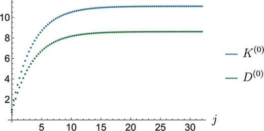
Fig. A.1.
Convergence of the wall correction factors with and . Here, is the reflection number.
Further, we must also ensure is large enough to accurately project cylindrical expressions onto the sphere surface. In Fig. A.2, we calculate the difference between the leading-order velocity on the sphere surface at obtained from the expressions in cylindrical coordinates (A.17) and the corresponding projection onto spherical coordinates via Equations (A.9) and (A.10) using either the first two () or three () non-zero terms in the spherical stream function series. Since we can exactly represent Poiseuille flow via a spherical stream function series with non-zero terms corresponding to and , this choice is the minimum required for the problem. However, if we impose the no-slip condition on the tube wall, and the particle is large enough to cause a substantial disturbance in the flow field, we must recruit higher order, even terms in . By including terms with , we recover a more accurate approximation of how the tube wall impacts the resulting leading-order deformation of the elastic particle. For describing pressure-driven channel flow around a rigid sphere under no applied body force, including the first three non-zero terms in the spherical stream function series ensures we can accurately apply both sets of boundary conditions simultaneously for . With larger , we would need to include higher terms in to reduce the error associated with the projection. We expect the MoR to converge exactly for .
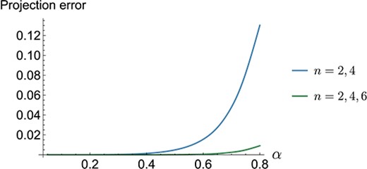
Fig. A.2.
The difference in predicted velocity on the undeformed particle surface with between the cylindrical terms and the projection to spherical coordinates in the method of reflections with . Graphs are shown including the first two () and first three () non-zero terms in the spherical stream function series.
B. Numerical model
We present a detailed overview of our non-linear ALE finite element model. The ALE method couples the Lagrangian solid problem and the Eulerian fluid problem. For clarity regarding these configurations, we again write and as the reference (Lagrangian) and current (Eulerian) configurations. For brevity, we present only the key details of the ALE problem set-up and refer the interested reader to Slyngstad (2017).
B.1 Lagrangian solid problem
To distinguish between the Eulerian presentation of the solid problem in Section 2 and the Lagrangian solid problem we specify the Lagrangian gradient as . It will also be useful to define the undeformed solid, fluid and boundary domains as and , respectively. The solid problem is then described by the balance of linear momentum,
where the first Piola-Kirchhoff stress tensor and . Again assuming the particle is incompressible, we have the further constraint (2.23).
B.2 Eulerian fluid problem
The Eulerian fluid problem is governed by the dimensionless Stokes equations (2.18–2.20). However, it is convenient to choose the undeformed reference configuration as the computational domain. To do this, we must transform the fluid equations to the reference configuration. We define the fluid mesh displacement associated with this transformation, and the associated deformation gradient tensor and Jacobian as
respectively. Making use of Nansen’s formula,
where and are the normal vectors in the deformed/reference configurations, respectively, we may write the stress balance across the fluid-solid interface (2.29) as
which is imposed on the undeformed particle boundary . Nansen’s formula (B.3) may also applied in conjunction with the divergence theorem to transform the Eulerian fluid equations to the reference configuration,
B.3 Arbitrary coupling
The solid displacement is physically motivated and provides a mapping between the undeformed reference and deformed configurations. The fluid mesh displacement has no physical interpretation. We require continuity () along the fluid-solid interface and do not permit normal fluid displacements along non-moving boundaries. Under these boundary conditions, the fluid mesh displacement extends any solid displacement into the fluid domain, and may be solved for using arbitrary governing equations. Previous studies have required satisfy Laplace’s equation, the equations of linear or non-linear elasticity, or the biharmonic equation Slyngstad (2017). In this study we opt to use the equations of linear elasticity such that
where and have no physical interpretation and in general do not have a consistent impact on problem convergence. After experimentation via a grid search, we opted to use and in this work.
B.4 Numerical implementation
In addition to the unknowns , we utilise several Lagrange multipliers to impose further constraints. These are, which ensures the mean solid displacement is zero, which is the particle’s translational velocity, which corresponds to the fluid traction acting on the solid, which ensures the mean fluid pressure is zero, and , which enforces the continuity of the fluid and solid displacement.
In order to solve an axisymmetric implementation of the FSI problem, we may extend the Cartesian equations to use a cylindrical coordinate system (Ruiz-Baier et al., 2022). There are several facets to consider in this extension. For example, we write the axisymmetric (cylindrical) divergence as
The axisymmetric gradient operator is identical to the Cartesian counterpart when applied to a scalar. When applied to vector, we have
which introduces further terms into the axisymmetric implementation. This can be seen, for example, in the determinant
The final change comes from the differential volume and surface area,
We now present the weak variational problem for the non-linear axisymmetric ALE FSI problem. We define the test functions associated with , respectively. Multiplying the governing equations by the respective test function, integrating and applying integration by parts the solid equations are
Similarly, the fluid equations are
The fluid mesh displacement equations are
We now use the various Lagrange multipliers to enforce their respective constraints. First, we impose the continuity of fluid velocity at the particle surface,
the continuity of fluid and solid displacement at the particle surface,
zero mean fluid pressure,
zero mean axial solid displacement,
and balance the fluid drag with the axial body force,
These constraints together describe a particle under an axial body force in equilibrium with the surrounding flow, and automatically calculates the equilibrium particle velocity.
B.5 Validation
To validate the solid solver we employ the method of manufactured solutions. Given a prescribed particle displacement, we use the solid governing equations to find analytical expressions for the required surface tractions and body force. These tractions and the body force are then used to drive the particle displacement in the numerical model, and the solution is compared with the analytical displacement field. Due to the complexity of the model and geometry, we choose the one-dimensional displacement field,
where determines the magnitude of the particle displacement as a fraction of the particle radius and is now the Lagrangian radial coordinate. Substituting (B.25) into the governing equations for the particle displacement, we obtain the corresponding surface tractions, , and body force,
where Lamé’s first parameter arises from the compressible neo-Hookean stress–strain relationship,
We note the switch from an incompressible particle to a compressible one is straightforward to implement and is necessary to obtain the above displacement field (B.25). We investigate the effect of increasing with no background flow () in Fig. B.1, presenting log-log plots of the -norm of the difference between the FEM displacement and (B.25). The typical error is of the order and increases with . For each , the error increases sharply as approaches , which is associated with the breakdown of the ALE method due to the large displacement.
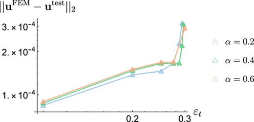
Fig. B.1.
-norm of the difference between the FEM displacement and the test analytical displacement averaged over the solid domain for varying displacement magnitudes . The simulations used the element sizes , and in the fluid, solid and boundary domains, respectively. These element sizes were chosen as the standard values and were used consistently within this study.
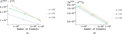
Fig. B.2.
Mesh refinement plots testing the solid, fluid and ALE solvers with fixed . Within each plot, we halve each element size and calculate the corresponding error. The middle data points correspond to the standard element size used in Fig. B.1. (a) Log-log plots of the -norm of the difference between the FEM displacement and the test analytical displacement for varying displacement magnitudes, . The average slope is . (b) Log-log plots of the norm of the absolute error between the FEM and MoR particle velocities. The average slope is .
To test the fluid and ALE solvers, we impose the traction (B.27) and include a background Poiseuille flow. We decrease such that the particle is effectively rigid to the imposed fluid stresses. Consequently, the fluid sees a rigid particle with inflated radius . The particle velocity of the inflated particle may then be compared with the MoR solutions for a particle with initial radius . In these comparisons, we acknowledge the MoR solutions are not exact, but expect the results for the particle velocity to be accurate to in all tested cases. We fix and investigate the effect of mesh refinement in Fig. B.2. We test the solid solver in Fig. B.2(a) similarly to Fig. B.1, and test the fluid and ALE solvers in Fig. B.2(b) by presenting the norm of the absolute error between the FEM and MoR particle velocities. For each , we include three mesh refinements and observe the convergence of the solid, fluid and ALE solvers. We note that the error in the particle velocity prediction appears to converge more slowly than the displacement since the particle velocity is also affected by the displacement predictions.
© The Author(s) 2019. Published by Oxford University Press on behalf of the Institute of Mathematics and its Applications. All rights reserved.
This is an Open Access article distributed under the terms of the Creative Commons Attribution License (
https://creativecommons.org/licenses/by/4.0/), which permits unrestricted reuse, distribution, and reproduction in any medium, provided the original work is properly cited.


