


Abstract
Limited-angle tomography is a highly ill-posed linear inverse problem. It arises in many applications, such as digital breast tomosynthesis. Reconstructions from limited-angle data typically suffer from severe stretching of features along the central direction of projections, leading to poor separation between slices perpendicular to the central direction. In this paper, a new method is introduced, based on machine learning and geometry, producing an estimate for interfaces between regions of different X-ray attenuation. The estimate can be presented on top of the reconstruction, indicating more reliably the separation between features. The method uses directional edge detection, implemented using complex wavelets and enhanced with morphological operations. By using convolutional neural networks, the visible part of the singular support is first extracted and then extended to the full domain, filling in the parts of the singular support that would otherwise be hidden due to the lack of measurement directions.
1. Introduction
X-ray tomography aims to recover the attenuation coefficient inside a physical body from a collection of radiographs recorded along different directions of projection. This study focuses on limited-angle tomography, where the directions of the lines in the dataset are severely restricted. Such cases appear in many important applications of X-ray tomography, for example, digital breast tomosynthesis (DBT) (Niklason et al., 1997; Dobbins III & Godfrey, 2003; Tao et al., 2004; Rantala et al., 2006; Vedantham et al., 2015; Loli Piccolomini & Morotti, 2016; Landi et al., 2017; Germana Landi et al., 2019), weld inspection (Haith et al., 2017; Silva et al., 2021), underwater pipeline inspection (Riis et al., 2018) and phase microscopy (Guo et al., 2021).
DBT is an enhanced form of mammography where one collects several X-ray images of a compressed breast within a limited angle of view. See Fig. 1(a) for an illustration of the DBT measurement geometry. This provides more information about the three-dimensional structure of the tissue and potentially leads to improved diagnosis of breast cancer.
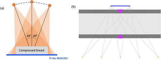
(a) Imaging geometry of DBT, based on collecting several radiographs of the compressed breast at various angles. Typically, the most extreme directions are |$\pm 20^{\circ }$| from the vertical, as shown in the image. While only three projections are depicted here, real DBT systems collect more (e.g. 15) images within the |$40^{\circ }$| angular range available. Limited-angle imaging geometry is forced by the compression of the breast against the detector plate. If the angle becomes too extreme, the rays passing through the tissue will not hit the detector. (b) Imaging geometry for X-ray inspection of weldings in pipelines used for example in process industry. Shown is a longitudinal cross-section of the pipe, with dark gray colour indicating metal. The purple area is the weld connecting two pieces of pipe together. Limited-angle imaging geometry is necessary as both the X-ray source and the detector need to be outside the long pipeline.
Long pipelines are used, for instance, in process and energy industries. They are often constructed by welding together several pieces of metal pipes. With welding, there is a risk of gas bubbles, cracks or other defects forming inside the weld. One can use limited-angle X-ray tomography for non-destructive testing of the welds with imaging geometry as shown in Fig. 1(b).
The inverse problem of limited-angle tomography is harder to solve than the full-angle case because it is much more ill-posed (Davison, 1983; Natterer, 1986; Kolehmainen et al., 2003; Siltanen et al., 2003). However, this ill-posedness has a particular geometric structure, revealed by microlocal analysis (Quinto, 1993; Frikel & Quinto, 2013). Consider imaging an object consisting of roughly homogeneous areas separated by crisp interfaces. Typical limited-angle reconstructions can recover the parts of the object boundaries that are tangented by X-rays used in the measurement. Other boundaries usually stretch out smoothly, offering no reliable information about the true location of the interface. In particular, separate objects in the target tend to merge together in the reconstruction along the central direction of projection. Reconstruction from limited-angle data has been done in many ways in the literature, for example with algebraic methods (Andersen, 1989), variational regularization (Delaney & Bresler, 1998; Sidky et al., 2006; Ritschl et al., 2011; Frikel, 2013; Chen et al., 2013b; Huang et al., 2016, 2018) and Bayesian inversion (Hanson & Wecksung, 1983; Kolehmainen et al., 2003; Rantala et al., 2006; Afkham et al., 2023).
We introduce a new, partly data-driven and partly geometric method for recovering interfaces between different areas of X-ray attenuation in the target. We show how complex wavelets and neural networks can be used to first detect the visible parts of the interfaces and then extend them to the invisible parts. Before going into details of our algorithm, we review the related methodology in the literature.
In recent years, deep learning has been used to improve the quality of computed tomography (CT) reconstructions in different ways (Adler & Öktem, 2017; Jin et al., 2017; Arridge et al., 2019; Wang et al., 2020). One successful approach is to use a neural network as a post-processing step to improve the quality of the CT reconstruction (Pelt et al., 2018). While this method can produce promising results in reducing noise or imaging artefacts, such post-processing neural networks are generally considered ‘black-box’. Additionally, such networks typically require large amounts of training data, which can be impractical in certain applications, for instance, in medical imaging. Also, the post-processing solution might not be optimal for severely ill-posed problems, where the quality of the initial reconstruction is extremely flawed.
An alternative approach is to combine analytical inverse problems algorithms with deep learning. These kinds of reconstruction techniques take advantage of the strengths of both variational regularization and deep learning. Having the explicit forward operator improves robustness and generalizability of the network, compared to previously mentioned ‘black-box’ neural networks. In addition, such model-based reconstruction reduces the amount of training data needed. This is due to the fact that the network has less parameters, and the forward operator encodes the imaging geometry so that it does not need to be learned (Adler & Öktem, 2017, 2018).
With modern machine learning methods, it has become possible to suppress streak artefacts with unprecedented efficiency. As shown in Bubba et al. (2019), it is possible to learn only the information which is not stably represented in the limited-angle tomographic data. The authors propose a hybrid framework with shearlets and a convolutional neural network for solving limited-angle CT problems. There, the network fills in only the missing shearlet coefficients, and the rest is done using rigorous inversion methods. Thus, the result can be seen as interpretable, as the network only affects a controlled part of the final reconstruction. We remark that the key difference between the present work and Bubba et al. (2019) is that here we aim to recover only interfaces between different domains. In Adler & Öktem (2018), the authors propose a deep learning framework for CT by unrolling a proximal-dual optimization method. In their Learned Primal-Dual (LPD) algorithm, convolutional neural networks replace the proximal operators. In Bubba et al. (2021), the authors unroll the iterations of a well-known iterative scheme and combine this with the convolutional nature of the limited-angle X-ray transform (and basic properties defining an orthogonal wavelet system) to derive a convolutional neural network where the operations of upscaling, downscaling and convolution are ‘prescribed’ by the wavelet system. In Andrade-Loarca et al. (2022), the authors combine microlocal analysis to the LPD algorithm and propose a scheme for joint reconstruction and wavefront set inpainting, enabling significant reduction of streak artefacts. Recently, shearlets and convolutional neural networks have successfully been used in image wavefront set detection, outperforming all conventional edge-orientation estimators and state-of-the-art data-driven methods (Andrade-Loarca et al., 2019).
Inherent in deep learning is the aforementioned ‘black-box’ problem; in other words, poor understanding of how did the algorithm arrive at the resulting reconstruction. Especially in medical imaging, it is often important to use algorithms that are as interpretable as possible. With this is mind, our proposed method aims to only learn the unstable parts of the boundaries, which can then be displayed as extra information, on top of a classical (non-learned) reconstruction.
We introduce a new algorithm for improved reconstruction: a data-driven and geometry-guided hybrid. See Fig. 3 for a summary of the method. We first compute an initial reconstruction of the target using a suitable algorithm, for example, Primal-Dual Fixed-Point (PDFP) method (Chen et al., 2013a) promoting frame sparsity, but any other algorithm providing a reasonable reconstruction should work. Due to the limited-angle imaging geometry, the reconstruction contains stretching artefacts.
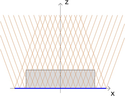
Idealized limited-angle imaging geometry we consider in our computational examples. We restrict to parallel-beam geometry. Shown here are the two extreme angles in our measurement model; we use a total of 50 directions distributed evenly in the angular variable between these two extremes. There is a significant difference in terms of imaging technology between our model and the two applications shown in Fig. 1, due to the fan-beam geometry used there. Namely, it is cumbersome to realize parallel-beam measurements with an X-ray source. However, the mathematics of wavefront sets is essentially the same, so our findings should apply with straightforward modifications.
Next, we aim to detect the stable parts of boundaries within the reconstruction. We transform the reconstruction using Dual-Tree Complex Wavelet Transform (DTCWT), which has directional selectivity oriented at |$\pm 15^{\circ }$|, |$\pm 45^{\circ }$| and |$\pm 75^{\circ }$|. From a theoretical perspective, DTCWT cannot resolve the wavefront set, as curvelet and shearlets do, but can provide reliable information on the singular support. However, the selective directional sensitivity at |$\pm 15$|, |$\pm 45$|, |$\pm 75$|, combined with nonlinear morphological operations in our data-driven framework, results in a robust six-angle edge detector, capable of automatically excluding streak artefacts. Our learned edge detection algorithm is independently applicable to a wide range of image processing tasks.
Using a neural network model, we can then learn the missing parts of the wavefront set in the framework of six oriented sub-bands, extending it beyond the scope of the limited-angle measurements. Our approach manages to ignore the streak artefacts and estimates the unstable parts of the boundaries of objects. Then, we can use this extended information about the wavefront set to form a boundary estimate that can be added as an overlay to the reconstruction.
We illustrate our method with computational examples using both simulated and real data. With simulated data, we work with parallel-beam geometry as shown in Fig. 2. This simplifying assumption helps in computational experiments as we can divide the 3D tomography problem defined in |$xyz$|-space into a stack of independent 2D problems posed in |$xz$|-planes determined by a constant value of |$y$|. The results are viewed by browsing through the |$xy$|-planes of the reconstructed volume by varying the |$z$|-coordinate. Our algorithm is especially useful when two or more objects have overlapping projections in the |$xy$|-plane, but are clearly separated in the |$z$|-direction. Such objects are typically merged together in traditional limited-angle reconstructions, but the approximately recovered wavefront set reveals the separation. With real data, the method is used with cone-beam geometry.
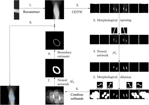
Workflow of the proposed method: (1) Compute an initial reconstruction. (2) Compute the finest scale complex wavelet coefficients for the six sub-bands and take their absolute value. (3) Clean the coefficients using morphological opening with appropriately oriented line structuring elements. (4) Give this to the first neural network, which thresholds the six sub-bands into a binary format. (5) Compute an initial guess of the microlocal prior, by dilating the binary sub-bands with specific directed structuring elements. (6) Combine the information in the six sub-bands by summation. (7) Give this initial guess to the second neural network, which estimates how the wavefront set extends, outputting a prediction of the full singular support. (8) Compute the morphological skeleton of the singular support, extracting its boundary. (9) Add this learned boundary estimate as an overlay on top of the reconstruction.
The structure of this paper is as follows. In Section 2, we go through the main mathematical background information necessary to understand the proposed method. In Section 3, we describe our proposed method for learned wavefront set extraction for limited-angle tomography. Then, in Section 4, we continue to explain the process of learning a microlocal prior. Next, in Section 5, we show the results of our proposed method for simulated (Sections 5.1, 5.2) and experimental data (Section 5.3). Finally, in Section 6, we end with some concluding remarks.
2. Mathematical background
In this section, we review basic concepts useful for the remaining of the paper. The definition of wavefront set, singular support and tomography is provided in Section 2.1; the CDTW transform is covered in Section 2.2; complex wavelet and total variation (TV) regularization methods are presented in Section 2.3. We conclude these mathematical preliminaries with an overview of the morphological operations needed later on in the computations in Section 2.4.
2.1 Wavefront set, singular support and tomography
Microlocal analysis is a powerful tool to study functions, operators and their singularities, in terms of their wavefront set. In the context of our work, microlocal analysis serves to predict which sharp features (singularities) of an image can be reconstructed in a stable way from limited data measurements. In limited-angle tomography, this translates to knowing that certain elements of the wavefront set of the X-ray attenuation coefficient are available, while information about the rest of the wavefront set is not present in any well-posed form. We recall briefly the definitions of singular support and wavefront set here for the convenience of the reader.
The wavefront set of a signal |$f \in L^{2}_{\text{loc}}(\mathbb{R}^{2})$| describes both the location |$x_{0}$| and the direction |$\theta _{0}$| of singularities. The signal |$f$| is smooth near |$x_{0}$| if there is a cutoff function |$\phi \in C^{\infty }_{c}$|, |$\phi (x_{0}) \neq 0$|, such that the Fourier transform of |$\phi f$| decays rapidly. That is,
The signal |$f$| has a singularity in |$x_{0}$| if for all cutoff functions |$\phi $|, the Fourier transform of |$\phi f$| does not decay rapidly. The set of all singularities of |$f$| is called the singular support and is denoted by |$\mathtt{singsupp}(f)$|. To define the orientation of the singularities |$x \in \mathtt{singsupp} (f)$|, we look for directions along which the localized Fourier transform |$\widehat{\phi f}$| does not decay rapidly.
Define the wavefront set of a function |$f$| as the set |$WF(f)(x_{0}, \alpha _{0})$| with location |$x_{0} \in \mathtt{singsupp} (f)$| and direction |$\alpha _{0}$|, such that for all cutoff functions |$\phi \in C^{\infty }_{c}$|, |$\phi (x_{0}) \neq 0$|, the localized Fourier transform |$\widehat{\phi f}(\xi )$| does not decay rapidly in any polar wedge |$W_{\delta } = \{(r,w):|w -\alpha _{0}| < \delta \}$|, where |$(r,w)$| are the polar coordinates in the frequency domain. The direction |$\alpha _{0}$| of a singularity |$x_{0} \in \mathtt{singsupp} {f}$| can be considered as the direction of maximum change of |$f$| at |$x_{0}$|. In particular, for a piecewise constant function having a jump along a Jordan curve |$\gamma $|, |$\mathtt{singsupp} (f)$| equals |$\gamma $| and |$WF(f)$| consists of pairs |$(x_{0}, N(x_{0}))$| with |$x_{0}\in \gamma $| and |$N(x_{0})$| the normal vector of |$\gamma $| at |$x_{0}$|.
Consider the continuous two-dimensional Radon transform |$\mathcal{R}f$| of a function |$f \in L^{1}(\mathbb{R}^{2})$|:
where |$L(\theta ,s) = \{ x \in \mathbb{R}^{2}: x_{1} \text{cos}(\theta ) + x_{2} \text{sin}(\theta ) = s \}$| is the line with normal direction |$\theta $| and signed distance from the orientation |$s$|. Given the Radon transform data |$\mathcal{R} f(\theta ,s)$| for |$(\theta ,s)$| arbitrarily near |$(\theta _{0}, s_{0})$|, one can reconstruct singularities of |$f$| stably with location |$x \in L(\theta _{0},s_{0})$| and direction |$\theta _{0}$|. In other words, a singularity |$(x_{0},\theta _{0})$| of |$f$| is visible from a limited-angle measurement if the line |$L(\theta _{0}, x_{0}\cdot \theta _{0})$| is recorded in the measurements. See Greenleaf & Uhlmann (1989), Quinto (1993), Frikel & Quinto (2013) and Frikel (2013) for references.
In (parallel-beam) limited-angle tomography, we know the Radon transform |$\mathcal{R} f (\theta ,s)$| for all |$s\in \mathbb{R}$| and for the angular range |$[\theta _{0}-\delta ,\theta _{0}+\delta ]$|, for some |$\theta _{0}\in \mathbb{R}$| and |$0<\delta <\pi $|. Then, the visible part of the wavefront set is |$WF(f)(x_{0}, \alpha )$|, for
In Fig. 4, we show an example of the visible part of the wavefront set for |$\delta =\pi /4$|, (45|$^{\circ }$|) and |$\delta =\pi /18$|, (20|$^{\circ }$|).
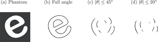
Demonstration of the visible part of the wavefront set in limited-angle tomography. (a) Digital phantom, where attenuation coefficient |$f(x)=0$| in the black area and |$f(x)=1$| inside the white character ‘e’. (b) Full singular support of |$f$|. (c) We simulated parallel-beam Radon transform data of |$f$| in the limited angular range |$-45^{\circ }\leq \theta \leq 45^{\circ }$|, calculated the filtered back-projection reconstruction, and determined the singular support using dual-tree complex wavelets. Which parts of the jump curves are missing? Those whose tangents are not parallel to any X-rays in the data. (d) Same as (c) but with more limited angular range |$-20^{\circ }\leq \theta \leq 20^{\circ }$|.
2.2 Complex dual-tree wavelet transform
While the concepts in the previous section are infinite-dimensional and of rather abstract nature, a central question is if it possible to access the visible part of the wavefront set in a practical manner. Multidimensional representation systems such as wavelets provide some insight.
The dual-tree complex wavelet transform consists of a complex-valued scaling function |$\phi $| and a complex-valued wavelet |$\psi $|. Consider a complex and analytic wavelet |$\psi (x)$|, given by
and associated with a high-pass filter |$H$|, and a complex and analytic scaling function |$\phi (x)$|, which is given by
and associated with a low-pass filter |$L$|. Note that |$\psi _{h}$| and |$\phi _{h}$| are the real parts of |$\psi (x)$| and |$\phi (x)$|, and |$\psi _{g}$| and |$\phi _{g}$| are the imaginary parts of |$\psi (x)$| and |$\phi (x)$|, respectively. For computational purposes, we use finitely supported wavelets and thus approximately analytic wavelets.
We denote the complex wavelet coefficients by |$d_{\nu } (j,n)\in{\mathbb C}$|, where |$j=0,\dots ,J$| represents the number of scales used in the complex wavelet representation and
represents the index of the six oriented sub-bands in each scale |$j$|. Note that |$j=0$| corresponds to the mother wavelet and |$j = J$| corresponds to the finest scale. See Fig. 5(b) for the frequency-domain content indexed by |$\nu $|.
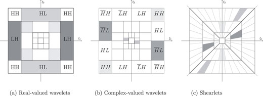
Frequency tilings of different multi-resolution transforms. (a) Real-valued wavelets are often understood to give horizontal, vertical and diagonal details. This can be seen in the approximate supports of the basis functions in the frequency domain. (b) The approximate supports of the Fourier transforms of the frame functions corresponding to the six sub-bands in the dual-tree complex wavelet transform. (c) Shearlets offer very detailed analysis of orientations using parabolic scaling and increasing numbers of orientations with finer scales. However, the benefits come with a computational cost.
To build intuition, the expression for the 2D wavelet in sub-band |$HH$| is obtained by
Note that this wavelet is oriented at |$-45^{\circ }$|. To obtain the 2D wavelet oriented at |$+45^{\circ }$|, which is the sub-band |$\overline{H} H$|, we compute |$\psi _{2}(x_{1},x_{2}) = \overline{\psi (x_{1})} \psi (x_{2})$|, where
In a similar manner, the six sub-bands of the 2D complex wavelets for each scale |$j$| are computed as follows:
Here |$n=(n_{1},n_{2})\in{\mathbb Z}^{2}$|. For discrete images of the size of power-of-two (which we consider throughout the paper), |$n_{1}$| and |$n_{2}$| range from |$0$| to |$2^{j}-1$|, depending on the scale |$j$|. In our computations, j will range from |$0$| to |$6$|, with |$0$| corresponding to the coarsest scale and |$6$| corresponding to the finest scale. We remark that the digital wavelet transform starts by computing the finest scale by applying filters to a pixel image. The calculation progresses towards coarser scales by repeatedly applying the filters to the low-pass sub-bands. For a more detailed look on the theoretical properties of the complex wavelet transform, please refer to Selesnick et al. (2005).
The complex wavelet coefficients are defined by
Here, the function |$f$| can be recovered from the coefficients by
where |$S$| is the frame operator
where |$T$| is the analysis operator and |$T^{\ast }$| is the synthesis operator corresponding to |$S$|. See Fig. 6 for an example of the absolute values of complex wavelet detail coefficients for all six sub-bands of the finest scale.
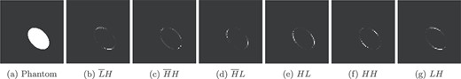
The first scale of complex wavelet detail coefficients of a phantom shown in (a). The orientations of coefficient sub-bands are denoted below each sub-band. Here, the absolute value of the complex-valued detail coefficients is shown.
The complex wavelet transform also gives rise to real-valued, final-level low-pass scaling coefficients, known as the approximation coefficients. They are given by
The motivation for using complex wavelets is that they offer a good compromise between directionality and computational cost. More precisely, real-valued wavelets offer only very limited information about the orientation of the edges in an image. On the other hand, curvelets (Candès & Donoho, 2004) and shearlets (Labate et al., 2005; Kutyniok & Labate, 2012) use parabolic scaling, along with rotation or shearing, to achieve remarkably accurate approximation properties for the wavefront set. However, for our purposes, the DTCW transform offers just the right balance between directionality and computational cost. See Fig. 5 for an illustration of the frequency content of the building blocks of these three types of transforms.
2.3 Inverse problems and regularization
After suitable discretization, the inverse problem of reconstructing a tomographic image |${\textbf{f}} \in \mathbb{R}^{n}$| based on X-ray measurements |${\textbf{m}} \in \mathbb{R}^{m}$| is modelled by
where |$A \in \mathbb{R}^{m \times n}$| is linear forward operator discretizing the Radon transform and |$\epsilon \in \mathbb{R}^{m}$| models additive Gaussian noise. We consider regularized solutions to the inverse problem (17), achieved by minimizing the following functional:
where |$R(\textbf{f})$| is the so-called regularization term, encoding some form of prior information which might be available on the solution, and |$\mu>0$| is the regularization parameter providing a balance between data fidelity and the a priori information. In particular the sparsifying effect induced by the |$\ell ^{1}$|-norm of some multidimensional representation system has been an active field of research over the last two decades, often leading to state of the art results for the inversion from limited data. Finally, in most tomographic problems, it is known a priorily that the desired image |$\textbf{f}$| is non-negative and including the constraint |$\textbf{f}\geq 0$| (meant component-wise) into (18) leads to superior reconstruction results.
We present below two classic choices for the regularizer |$R(\textbf{f})$|, wavelet-based and total variation regularization, which have been a popular choice for sparsity-based regularization of inverse problems.
2.3.1 Complex wavelets regularization
With complex wavelet regularization the minimization problem (18) reads as follows:
where, in this case, the term |$\| W_{\mathbb{C}}{\textbf{f}}\|_{1}$| promotes solutions having sparse representation in the wavelet basis. Analogous regularization was used in Purisha et al. (2017), but with real wavelets instead of complex-valued.
The Primal-dual fixed-point algorithm, described by (Chen et al., 2013a), can be used to iteratively solve the minimization problem (19). The algorithm is given by
where |${\mathcal{G}}({\textbf{f}}) = \frac{1}{2} \|A{\textbf{f}} -{\textbf{m}}\|_{2}^{2}$|, and |$\mu> 0 $| is the regularization parameter and |$\tau $| and |$\lambda $| are positive parameters that need to be suitably chosen for convergence. In particular, |$0<\lambda < \frac{1}{\lambda _{\text{max}}(W_{\mathbb{C}}(W_{\mathbb{C}})^{T})}$|, where |$\lambda _{\text{max}}$| is the maximum eigenvalue, and |$0<\tau <2/\tau _{\text{lip}}$|, where |$\tau _{\text{lip}}$| is the Lipschitz constant for |$\mathcal{G}({\textbf{f}})$|. The soft-thresholding operator |$\mathcal{T}$| is defined radially for complex-valued inputs as
In equation (20), the non-negative quadrant is denoted by |$C = \mathbb{R}^{N^{2}}_{+}$| and |$\mathbb{P}_{C}$| is the Euclidean projection, that is, the operator |$\mathbb{P}_{C}$| replaces any non-negative elements in the input vector by 0s.
2.3.2 Total Variation regularization
Another way to solve the inverse problem (17) of reconstructing a tomographic image, |${\textbf{f}} \in \mathbb{R}^{n}$|, based on X-ray measurements, |${\textbf{m}} \in \mathbb{R}^{m}$|, is to minimize the functional
where |$L$| is the finite difference matrix and the |$\ell ^{1}$|-norm of a vector |${\textbf{x}} \in \mathbb{R}^{n}$| is defined as usual. The above problem is derived from the following continuous formulation:
where |$ \text{TV}(f)$| is the total variation (TV) regularization term over the domain |$\varOmega $|, given by
TV regularization amounts to enforcing gradient sparsity, thus removing unwanted details whilst preserving important features such as edges.
To solve the discrete minimization problem (22), we use the Primal-dual ascent-descent algorithm with TV regularization (presented by Bredies (2014)), modifying the implementation for tomographic reconstruction. In the results presented in Section 5, this algorithm is referred to as TV.
2.4 Morphological operations
We conclude this section by recalling some key definitions of morphological operations (Gonzalez & Woods, 2018), which, in this work, are used to clean and pre-process greyscale and binary data. In mathematical morphology, we consider the original image as the object |$\mathcal{D}\subset \mathbb{Z}^{2}$|. A structuring element |$S\subset \mathbb{Z}^{2}$| is a pre-defined binary image that is used to probe the object |$\mathcal{D}$|, and conclude how it fits the shapes of the object.
The morphological dilation operation can be used to ‘grow’ objects in a binary image. The shape and size of the structuring element |$S$| defines the extent of the dilation. The dilation operation is defined as
where |$\mathcal{D}_{s} = \{ d+s | d \in \mathcal{D}, s \in S\}$| is the translation of |$\mathcal{D}$| by the structuring element |$s$|.
On the other hand, morphological erosion thins out objects in a binary image. It is the dual operation of dilation. The erosion operation is defined as
The morphological opening operation removes small details from the object but preserves the shape and size of larger objects. The opening of |$\mathcal{D}$| by |$S$| is defined as
where |$\mathcal{D} \ominus S$| is the morphological erosion of |$\mathcal{D}$| by |$S$|, and |$\oplus $| is the dilation operation of the result by |$S$|. The opening of |$\mathcal{D}$| by |$S$| can be seen as the union of all the translations of |$S$| so that it fits within the object |$\mathcal{D}$|:
where |$ \mathcal E_{\mathcal D}=\{z\in \mathbb Z^{2}:\ S_{z} \subseteq \mathcal{D}\}$|.
The morphological skeleton operation extracts the centreline of the objects in a binary image while preserving its topology. The operation transforms the object |$\mathcal{D}$| to 1-pixel wide curved lines while not changing the essential structure. It can be expressed in terms of morphological erosions and openings:
where |$(\mathcal{D} \ominus kS)$| expresses |$k$| successive erosion operations and |$K= \max \{k | (\mathcal{D} \ominus kS) \neq \emptyset \}$| denotes the last step before the object |$\mathcal{D}$| erodes to an empty set.
Morphological operations can be extended for greyscale images. In that case, |$\mathcal{D}$| in formula (28) is a greyscale pixel image. In greyscale morphology, images |$d$| are functions mapping the Euclidean space |$E$| into |$\mathbb{R} \cup \{-\infty ,\infty \}$|. That is, |$ d: E \rightarrow \mathbb{R} \cup \{-\infty ,\infty \}. $| The greyscale structuring elements are also functions mapping Euclidean space into |$\mathbb{R} \cup \{-\infty ,\infty \}$|.
Denote an image by |$d(x)$| and a structuring function by |$b(x)$|. Then, the dilation operation is defined as
where |$\sup $| denotes the supremum. The erosion of |$d$| by |$b$| is given by
while the opening and closing are given by
If |$b(x)=\mathbf{1}_{B}(x)$| is the indicator function of the set |$B$| and |$d(x)=\mathbf{1}_{D}(x)$| is the indicator function of the set |$D$|, we have
Similar formulas hold for dilation |$d \oplus b$| and erosion |$d \ominus b$|.
3. Learned wavefront set extraction
In limited-angle tomography, the reconstructed image typically fails to reproduce certain parts of the wavefront set of the original target, as explained in Section 2.1. This is often accompanied by severe stretching artefacts in the reconstruction along the central direction of projection, as illustrated in Fig. 7.
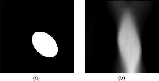
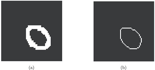
(a) Elliptical computational phantom with constant attenuation and zero background. (b) PDFP reconstruction with complex wavelet regularization from 50 X-ray projection images over a 40-degree opening angle. The central direction of projection is vertical. Note the vertical elongation or stretching of the ellipse in the reconstruction. This is a typical artefact in limited-angle tomography.
Our goal is to fill in the missing parts of the wavefront set by machine-learning the geometric rules of how the known parts of the wavefront set extend into the unknown parts. See Fig. 8 for the geometric idea behind this microlocal prior. After we have the full wavefront set available, we can use it to form a boundary estimate of features.
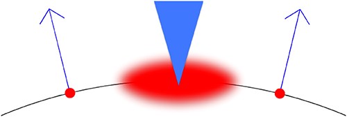
The geometric idea behind our microlocal prior. Assume we know two elements of the wavefront set, located spatially at the two red dots and having the directions indicated by the two blue arrows. We work with piece-wise constant attenuation coefficients having reasonably regular boundary curves (shown as the black arc here) between the constant domains. Then we know that there should be another element in the wavefront set with a spatial location somewhere in the area shown as blurred red, and with direction within the range indicated with the blue triangle.
We compute the aforementioned boundary estimate in several steps, including the application of two distinct convolutional neural networks. The first neural network learns to extract the known part of the wavefront set by transforming morphologically opened complex wavelet coefficients to a binary form. The second neural network learns to predict the complete singular support from the incomplete wavefront set that has been morphologically dilated. We will discuss the second network, among with the operations related to it, in Section 4.
3.1 Complex wavelet coefficients of a limited-angle reconstruction
We simulate a parallel-beam limited-angle sinogram with 50 projection directions and a 40-degree opening angle. The opening angle of |$40$|-degrees was chosen as it arises in the practical application of 3D mammography. Further, we compute a reconstruction using, for example, variational optimization with complex wavelet regularization as described in Section 2.3.1. Other regularised approaches can be used as well, as the choice of reconstruction algorithm does not drastically affect the known part of the wavefront set. Because of the limited-angle imaging geometry, the features in the reconstruction are stretched along the central direction of projection, as can be seen in Fig. 7.
First, we want to extract the wavefront set (see Section 2.1) from the reconstruction. This is accomplished by picking out a discrete approximation of the wavefront set by using the finest scale of dual-tree complex wavelet coefficients |$d_{\mathbb{\nu }}(j,n_{1},n_{2})$|, where |$j = 6$|, |$n=(n_{1},n_{2})\in{\mathbb Z}^{2}$| and |$\nu \in \mathcal I$| is as described in Section 2.2. The amount of scales available is based on the size of the image.
Then, we take the absolute value of the coefficients:
A demonstration can be seen in Fig. 9(a).
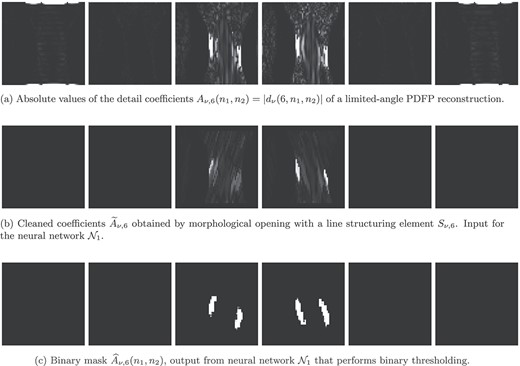
Going from (a) the imperfect and approximate wavefront set provided by DTCW coefficients into a robust wavefront set estimator. The technique involves two nonlinear steps: (b) morphology followed by (c) learning. The sub-band indices from the left to right are: |$\overline{L}H, \overline{H}H, \overline{H}L, HL, HH,LH$|.
Due to the limited-angle data, we observe nonzero complex wavelet coefficients mainly in sub-bands |$d_{\overline{H}L}(6,n_{1},n_{2})$| and |$d_{HL}(6,n_{1},n_{2})$|, while sub-bands |$d_{\overline{L}H}(6,n_{1},n_{2})$|, |$d_{\overline{H}H}(6,n_{1},n_{2})$|, |$d_{HH}(6,n_{1},n_{2})$| and |$d_{LH}(6,n_{1},n_{2})$| contain no information beyond noise. This is because the reconstruction from a limited-angle sinogram can only encode information about certain directions of the wavefront set, as explained in Section 2.1.
3.2 Morphological opening of the complex wavelet coefficients
Due to stretching artefacts and imperfect measurements, the complex wavelet coefficients available in sub-bands |$d_{\overline{H}L}(6,n_{1},n_{2})$| and |$d_{HL}(6,n_{1},n_{2})$| are noisy. Therefore, we improve this information of the wavefront set using two nonlinear steps: grayscale morphology followed by learning.
To extract useful information about the complex wavelet coefficients, we use the morphological opening operation on the absolute values of the complex wavelet coefficients. First, we set sub-bands |$d_{\overline{L}H}(6,n_{1},n_{2}), d_{\overline{H}H}(6,n_{1},n_{2}), d_{HH}(6,n_{1},n_{2})$| and |$d_{LH}(6,n_{1},n_{2})$| to zero. For the remaining two sub-bands |$d_{\overline{H}L}(6,n_{1},n_{2})$| and |$d_{HL}(6,n_{1},n_{2})$|, we perform morphological opening with oriented line structuring elements |$S_{\nu ,6}$|:
where |$A_{\nu ,6}$|, defined in equation (35), is a grayscale image considered as a function |$A_{\nu ,6}:{\mathbb Z}^{2}\to [0,1]$|. The line structuring elements |$S_{\nu ,6}$| are the binary images shown in Fig. 10 and are considered as a function |$S_{\nu ,6}:{\mathbb Z}^{2}\to \{0,1\}$|. For our limited-angle problem, we use structuring elements |$S_{\overline{H}L,6}$| and |$S_{HL,6}$|, since we perform opening for sub-bands |$d_{\overline{H}L}(6,n_{1},n_{2})$| and |$d_{HL}(6,n_{1},n_{2})$|. The result is illustrated in Fig. 9(b).

Now, one would think that hard-thresholding of the opened sub-bands as follows:
would give binary indicators for the discrete wavefront set. This would be the case if we had a good threshold |$\epsilon>0$| available. However, in practice, imperfect knowledge of the noise amplitude and the absence of ground truth makes it difficult to design an automatic method for choosing the threshold. Therefore, we resort to learning the thresholding process.
3.3 Learning the binary mask
We use a convolutional neural network |$\mathcal{N}_{1}:\mathbb{R}^{{\mathbb Z}^{2}\times \mathcal I}\to [0,1]^{{\mathbb Z}^{2}\times \mathcal I}$| to learn the binary indicators for the discrete wavefront set in the two sub-bands |$d_{\overline{H}L}(6,n_{1},n_{2})$| and |$d_{HL}(6,n_{1},n_{2})$|. The input of neural network |$\mathcal{N}_{1}$| is the tensor |$\widetilde A=(\widetilde A_{\nu ,6}(n))_{n\in{\mathbb Z}^{2},\nu \in \mathcal I}$| obtained from equation (36) and the network maps it to |$\widehat A=(\widehat A_{\nu ,6}(n))_{n\in{\mathbb Z}^{2},\nu \in \mathcal I}$|, that is,
The training of the neural network uses the morphologically opened complex wavelet coefficients |$\widetilde{A}_{\overline{H}L,6}(n_{1},n_{2})$| and |$\widetilde{A}_{HL,6}(n_{1},n_{2})$|. After the network |$\mathcal{N}_{1}$| performs the thresholding, it outputs a binary mask with ones indicating the location of the wavefront set. See Fig. 9(c) for an example result.
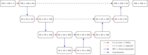
We implement neural network |$\mathcal{N}_{1}$| as a convolutional autoencoder with residual connections, as inspired by the U-net (Ronneberger et al., 2015), which has a track record of good empirical performance. In more detail, for the encoder and decoder parts of the network, we use convolution kernels of size |$3 \times 3$|, stride of size 1, and rectified linear unit (ReLU) activation functions. After each convolutional layer, we perform batch normalization, followed by down- or up-sampling. We use skip connections to join the encoder and decoder parts of the network to improve training. For the last layer, we use a |$1 \times 1$| convolution with a sigmoid activation. See the detailed architecture in Fig. 11. The best results were achieved by using the dice coefficient loss function given by
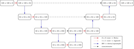
Network architecture of |$\mathcal{N}_{1}$|.
where |$\overline{A}$| denotes the ground truth values and |$\widehat{A}$| the network predictions.
The training inputs are generated as follows. We first generate 5000 two-dimensional phantoms of size |$128 \times 128$| with ellipse shapes that have varying radius, eccentricity, tilt and position. For each phantom, we consider 50 X-ray measurements over a |$40$|-degree opening angle, spanning from |$70$| to |$110$| degrees. We add |$5 \%$| Gaussian noise to the measurement sinogram. Then, we compute the reconstruction of each phantom using the PDFP algorithm with complex wavelet regularization. Next, we compute the absolute values of the complex wavelet coefficients, |$A_{\nu ,6}(n_{1},n_{2})$|, of each reconstruction. We set sub-bands |$A_{\overline{L}H,6}(n_{1},n_{2}), A_{\overline{H}H,6}(n_{1},n_{2}), A_{HH,6}(n_{1},n_{2})$| and |$A_{LH,6}(n_{1},n_{2})$| to 0. We perform morphological opening of the sub-bands |$A_{\overline{H}L,6}(n_{1},n_{2})$| and |$A_{HL,6}(n_{2},n_{2})$| by using formula (36). These morphologically opened sets of sub-bands |$\widetilde{A}_{\nu ,6}$| serve as the training inputs.
The corresponding ground truth values are generated as follows. First, we compute the absolute value of the complex wavelet coefficients of the ground truth phantoms. We again set sub-bands |$d_{\overline{L}H}(6,n_{1},n_{2}), d_{\overline{H}H}(6,n_{1},n_{2}), d_{HH}(6,n_{1},n_{2})$| and |$d_{LH}(1,n_{1},n_{2})$| to 0. We perform morphological opening on sub-bands |$d_{\overline{H}L}(6,n_{1},n_{2})$| and |$d_{HL}(6,n_{1},n_{2})$| using (36) to obtain |${\widetilde{A}}_{\overline{H}L,6} (n_{1},n_{2})$| and |${\widetilde{A}}_{HL,6} (n_{1},n_{2})$|. Then, we convert the data into a binary form by thresholding sufficiently large values of the morphologically opened coefficients to |$1$| and the rest are set to |$0$|. That is, in training of neural network |$\mathcal{N}_{1}$|, the ground truth data are obtained using the formula
using a suitably chosen |$\epsilon>0$|.
The training input and output datasets were of size |$5000 \times 128 \times 128 \times 6$| each. During training, 500 training set examples were used as the validation set.
4. Learned microlocal prior
In the previous section, we explained how to extract the known part of the wavefront set from a limited-angle tomography reconstruction. In this section, we will go through the rest of the steps in order to learn a boundary estimate. See Fig. 3 for a summary of the entire workflow of our proposed method.
The basic idea behind our microlocal prior is based on the assumption of the smoothness and bounded curvature of the singular support of the X-ray attenuation coefficient. When a part of a wavefront set is detected in a sub-band, the smooth singular support curve is locally oriented approximately along a piece of straight line oriented in the direction designated for that sub-band. Imagine traveling along the line. Eventually, the singular support is bound to turn outside the orientation range of the sub-band you are on, as the interfaces between areas of different attenuation are closed curves. Then the line ends abruptly. But there is a continuation of it on one of the two neighboring sub-bands, depending on the direction of the turn. The representation of the singular support continues there as an almost straight line (along an orientation 30 degrees rotated from where you started), until another inevitable turn is forcing a jump to yet another sub-band. The structuring elements shown in Fig. 12 are designed so as to capture the locations in a neighboring sub-band where the continuation can go.
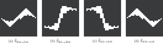
The custom-made directional structuring elements |$\widetilde{S}_{\nu \rightarrow \nu ^{\prime }}$| we use for our specific limited-angle measurement geometry.
We learn the boundary estimate with a second neural network |$\mathcal{N}_{2}$|, using the output of the first neural network |$\mathcal{N}_{1}$|. In order to do so, we first approximate the microlocal prior by morphological dilation. The details of the steps are explained in the sections below.
4.1 Approximation of the microlocal prior by morphological dilation
Now, we extend the wavefront set information from the two available sub-bands (see Fig. 13a) to the remaining four sub-bands. We begin by using morphological dilation, as explained in Section 2.4, to compute an initial guess for the location of non-zero coefficients. As the structuring elements for the operation, we have designed custom-made directional structuring elements that are able to estimate the location of the wavefront set based on a neighbouring sub-band. The structuring elements |$\widetilde{S}_{\nu \rightarrow \nu ^{\prime }}$|, |$\nu ,\nu ^{\prime }\in \mathcal I$| that we use for our specific limited-angle measurement geometry are shown in Fig. 12. These structuring elements are designed so that the elements (a) and (b) in Fig. 12 are the rotated and scaled images of the set
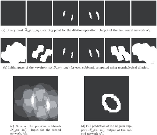
Learning to fill in the incomplete singular support from the wavefront set of six complex wavelet coefficient sub-bands, extending it to the entire domain. The sub-band indices from left to right are as follows: |$\overline{L}H, \overline{H}H, \overline{H}L, HL, HH,LH$|.
and the elements (c) and (d) are the rotated and scaled images of the set
The design is motivated by the assumption that the unknown object may have a discontinuity on a curve |$\gamma $| whose curvature is bounded. For example, the unknown object corresponding to function |$f$| may be a sum of the indicator function of a smooth domain |$D$| multiplied by a smooth function |$f_{1}$| and a smooth function |$f_{2}$|:
and |$\gamma :[-1,1]\to \mathbb{R}^{2}$| is a path satisfying |$\gamma ([-1,1])\subset \partial D$|. Let us consider the case when the path |$\gamma $| is parametrized as |$\gamma (s)=(s,h(s))$|, |$s\in [-1,1]$|, where |$h:[-1,1]\to \mathbb{R}$| is a function that satisfies |$h(0)=0$| and |$h^{\prime}(0)=0$|. Moreover, assume that the normal vector of |$\gamma (x)$| turns clockwise when |$s>0$| and |$s$| grows. Then for |$s>0$| the second derivative of |$h$| satisfies |$ h^{\prime\prime}(s)<0$|. If we also have |$0> h^{\prime\prime}(s)\ge -1$|, then |$\gamma ([0,1])\subset S^{-}$|. When |$s<0$|, we assume that the normal vector of |$\gamma (x)$| turns clockwise when |$-s$| grows and that |$0<h^{\prime\prime}(s)\le 1$|, in which case |$\gamma ([-1,0])\subset S^{-}$|. Note that for example the structuring element |$\widetilde S_{\overline H L\to \overline H H}$| corresponds to predicting the points |$x=(x_{1},x_{2})$| on the discontinuity |$\partial D$| with a normal vector |$\nu (x)$| of |$\partial D$| such that there exists a nearby point |$\tilde x=(\tilde x_{1},\tilde x_{2})\in \partial D$| with a normal vector |$\nu (\tilde x)$| such that |$\nu (x)$| is a vector close to |$\nu (\tilde x)$| that has been turned in the clockwise direction (see Fig. 8).
The approximation of the microlocal prior is done as follows using the above structuring elements. We make no changes to the sub-bands |$\overline{H}L$| and |$HL$|, since we have already extracted the wavefront set for these sub-bands in the previous steps. That is,
To get the wavefront set estimate for the adjacent sub-bands |$\overline{H}H$| and |$HH$|, we dilate sub-bands |$\overline{H}L$| and |$HL$| with the structuring elements |$\widetilde{S}_{\overline{H}L \rightarrow \overline{H}H}$| and |$\widetilde{S}_{HL \rightarrow HH}$|, respectively. That is,
Next, for sub-bands |$\overline{L}H$| and |$LH$|, we treat the once dilated sub-bands |$\overline{H}H$| and |$HH$| as the objects for the dilation with structuring elements |$\widetilde{S}_{\overline{H}H \rightarrow \overline{L}H}$| and |$\widetilde{S}_{HH \rightarrow LH}$|, respectively. That is,
See Fig. 13(b) for dilated sub-bands |$D_{\nu ,6}(n_{1},n_{2})$|.
Then, we can combine the wavefront set estimates in the sub-bands |$D_{\nu ,6}(n_{1},n_{2})$| to form an initial guess of the singular support (see Section 2.1). That is, we sum all six binary sub-bands together:
We now have a coarse starting point of the full wavefront set |$D^{+}_{\nu ,6}(n_{1},n_{2})$| for the network |$\mathcal{N}_{2}$| to refine. See Fig. 13(c) for an example.
4.2 Learning to extend the wavefront set into the entire domain
We want to learn to refine the wavefront set estimate with neural network |$\mathcal{N}_{2}$|, based on the combination of the approximations provided by the dilation operation. The network |$\mathcal{N}_{2}$| outputs a prediction of the full wavefront set |$\widehat{D}^{+}_{\nu ,6}(n_{1},n_{2})$|, extending it to the full domain. We use a convolutional neural network |$\mathcal{N}_{2}:\mathbb{R}^{{\mathbb Z}^{2}\times \mathcal I}\to [0,1]^{{\mathbb Z}^{2}\times \mathcal I}$|, where the input of |$\mathcal{N}_{2}$| is the tensor |$D^{+}=(D^{+}_{\nu ,6}(n))_{n\in{\mathbb Z}^{2},\nu \in \mathcal I}$| and the network maps it to |$\widehat D^{+}=(\widehat D^{+}_{\nu ,6}(n))_{n\in{\mathbb Z}^{2},\nu \in \mathcal I}$|. That is,
See Fig. 13(d) for an example output.
For neural network |$\mathcal{N}_{2}$|, we use a similar architecture as for network |$\mathcal{N}_{1}$|, however, here batch normalization is not used in the training (see Fig. 14). Otherwise, the training scheme and use of loss function were identical to that of network |$\mathcal{N}_{1}$|. See Section 3.3 for a more detailed explanation.
Network architecture of |$\mathcal{N}_{2}$|.
To get the training inputs for network |$\mathcal{N}_{2}$|, we use the same phantoms as with network |$\mathcal{N}_{1}$|. We perform morphological dilation (as explained in Section 4.1) on thresholded ground truth sub-bands |$\overline{A}_{\nu ,6}(n_{1},n_{2})$| (see equation 36) to obtain the approximations for the wavefront set |$D_{\nu ,6} (n)$| in each sub-band. Then, we add the sub-bands together, resulting in |$D^{+}_{\nu ,6} (n)$|. These act as the training inputs for |$\mathcal{N}_{2}$|.
The corresponding ground truth values are computed from the ground truth phantoms, where we have the full wavefront set information available in all of the sub-bands. We simply take the absolute value, morphologically open, combine the sub-band information to form the singular support and threshold the data to a binary form. These serve as the ground truth values in the training. The training datasets were of size |$5500 \times 128 \times 128$|, from which we used 500 samples for validation.
4.3 Boundary estimate
Then, we can compute the boundary of the singular support estimate |$\widehat{D}^{+}_{\nu ,6}(n_{1},n_{2})$| using the morphological skeleton operation described in equation (29) of Section 2.4. See Fig. 15 for the predicted full singular support and the corresponding skeleton. Finally, this learned boundary estimate can be used as an overlay for the reconstruction. See Section 5 for final results.
(a) The learned singular support |$\mathtt{singsupp} ( \widehat{D}_{\nu ,6})$| and (b) its boundary estimate.
5. Results
We tested the proposed method with different reconstruction algorithms for a simulated 3D-phantom (see Sections 5.1–5.2) and a simple real data measurement (Section 5.3). The reconstructions are computed using tomosynthesis, complex wavelet-based regularization (using PDFP) and TV regularization.
5.1 Reconstructions in the xz-plane with simulated measurements
For testing our proposed method, we created a three-dimensional phantom consisting of three |$L^{p}$| -balls in a constant background (see Fig. 16a). Here, the definition of the |$y \in \mathbb{R}^{2}$|-centred |$L^{p}$|-ball is as follows:
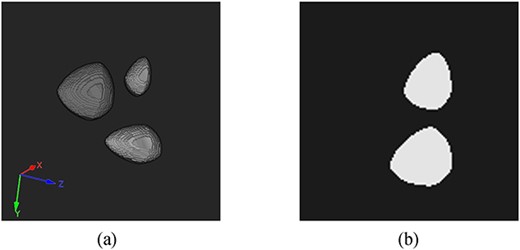
(a) Computational 3D phantom of size |$128 \times 128 \times 128$|: three |$L^{p}$| -balls, where |$p=1.5$|, with constant inclusion values (0.6, 0.8, and 1) in a 0-valued background. (b) Modified slice of the 3D phantom, where inclusions are vertically close together, making it particularly challenging for limited-angle tomography reconstruction.
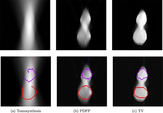
Comparisons of reconstructions with the corresponding learned boundary estimates for a modified |$xz$|-slice, where the inclusions are vertically close to each other. Reconstructions are computed using (a) tomosynthesis, (b) PDFP with complex wavelet regularization (1000 iterations) and (c) TV regularization (|$\alpha =5\times 10^{-5}$|, 10 000 iterations). On the bottom row, the learned boundary estimate is added to each corresponding reconstruction as an overlay. Imaging geometry: parallel beam, 40-degree opening angle (70–110), 50 projections, Poisson noise. The dotted line indicates the column plotted in Fig. 18.
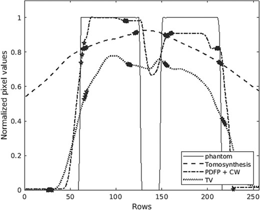
Column 160 of phantom (Fig. 16b) and its different reconstructions presented in Fig. 17. Because of the limited-angle geometry, stretching artefacts make it difficult to see the two separate inclusions in the reconstructions. The markers represent the learned boundary estimates, separating the actual features from artefacts.
where |$r$| is the radius and the weighted |$p$|-norm is defined as
where |$a=(a_{1},a_{2}).$| In the phantom, we had the following parameters: |$p=1.5$|, the weights |$a_{j}$| were picked from the interval |$[1,1.6]$|, and the radii were picked from the interval |$[0.2,0.3]$|. We chose to have |$L^{p}$|-balls in the test set, since they are convex sets with smooth boundaries but have curvatures changing in ways not straightforwardly predicted by elliptical shapes.
First, we simulated X-ray measurements of the phantom using a parallel-beam imaging geometry of a 40-degree opening angle with 50 projection images. We added |$5\%$| Gaussian noise to the sinograms. We computed reconstructions slice-by-slice, separately for each |$xz$|-plane, treating each slice as an independent 2D tomographic reconstruction problem.
Additionally, we created a modified slice with two of the |$L^{p}$| -balls vertically aligned and close together (see Fig. 16b). We added simulated noise by assuming a photon count of |$10\ 000$| in the pixel where the X-rays were not attenuated at all. Then we approximated Poisson noise by adding normally distributed random noise with an appropriate standard deviation. We note that with lower photon counts it would be advisable to use Kullback–Leibler data discrepancy, but here for simplicity, we just use Gaussian.
Following the workflow explained in Fig. 3, we learn the boundary estimate for each |$xz$|-slice. The learned boundary estimate is then overlaid on the corresponding reconstruction, to indicate the extent of boundaries of the stretched features in the reconstruction. See Figs 17 and 18 for reconstructions of the modified slice and the corresponding learned boundary estimates. For the original |$xz$|-slices of the test phantom, a selection of the complex wavelet and TV regularized reconstructions with boundary estimates are shown in Fig. 19. Also, the tomosynthesis reconstruction is shown here for comparison.
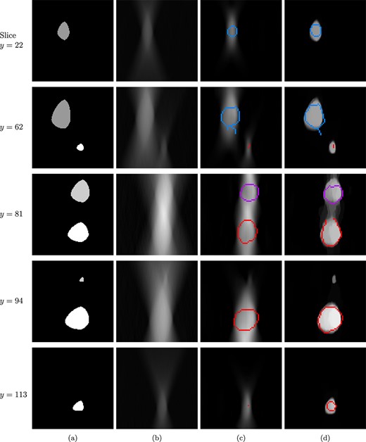
Different |$xz$|-slices through the three-dimensional test phantom shown in Fig. 16(a). In the model, |$xz$|-slices are vertical (perpendicular to the detector surface). In our simplified assumption of parallel-beam geometry, there is an independent limited-angle tomography problem restricted to each |$xz$|-slice. (a) Ground truth slice. (b) Tomosynthesis reconstruction. (c) PDFP reconstruction using complex wavelet regularization (100 iterations) with learned boundary estimate. (d) TV-regularized reconstruction (5000 iterations) with learned boundary estimate. Compare the boundary curves to the true boundaries of features shown in column (a).
5.2 Reconstructions in the xy-plane with simulated measurements
For a three-dimensional phantom, after independently computing the reconstructions and the boundary estimates for each of the |$xz$|-slices separately (see Section 5.1), we can stack the reconstruction results back together to form a volume. Then, we can slice the reconstructed volume in the |$xy$|-direction. We present the results as |$xy$|-slices with a selection of different |$z$|-values. The reconstruction results of several |$xy$|-slices of the |$L^{p}$|-ball test phantom are shown in Fig. 20.
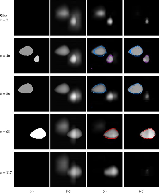
Different |$xy$|-slices through the three-dimensional test phantom of Fig. 16(a) and through 3D-volumes achieved by stacking 2D-reconstructions from |$xz$|-planes. In the model, |$xy$|-slices are parallel to the detector surface. (a) Ground truth slice. (b) Tomosynthesis. (c) PDFP reconstruction using complex wavelet regularization with learned boundary estimate. (d) TV-regularized reconstruction (5000 iterations) with learned boundary estimate. Note that one can deduce from the boundary curves that the grey features in the top and bottom images of column (c) are artefacts.
5.3 Reconstruction with experimental data
We created a physical test phantom consisting of two plastic pieces, as we wanted to verify that the method works for experimental data as well. We measured experimental data of the phantom at the University of Helsinki Industrial Mathematics Computed Tomography Laboratory, using a custom-built cone-beam CT scanner with a Hamamatsu Photonics C7942CA-22 flat-panel detector and an Oxford Instruments XTF5011 X-ray tube with a Mo target. See Fig. 21(a) for the experimental setup and the physical test phantom.
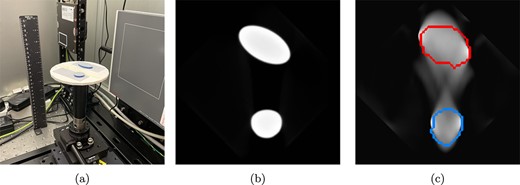
(a) The measurement set-up in the X-ray lab, (b) the PDFP reconstruction (1000 iterations) using full-angle data and (c) the PDFP reconstruction (1000 iterations) with limited-angle data together with the learned boundary estimate. The reconstruction is stretched, making it unclear how many separate objects there are. The boundary estimate reveals us the answer: two.
We collected measurements over 360 degrees, resulting in 721 projection images at intervals of 0.5 degrees. The measurements were collected using a tube voltage of 45 kV, a tube current of 1.0 mA and a detector exposure time of 1200 ms for each projection. From the full data, we sub-sampled 80 measurements over a 40-degree opening angle to create the desired limited-angle dataset. The experimental data was processed using the HelTomo Matlab toolbox (Meaney, 2022). We used the PDFP algorithm with complex wavelet regularization to compute reconstructions for the full and limited-angle data. Following the proposed method, we computed the learned boundary estimate for the limited-angle case. See Fig. 21(c) for the limited-angle reconstruction result and Fig. 21(b) for the full-angle reconstruction as comparison.
6. Conclusion
We introduced a new method for estimating the wavefront set of an X-ray attenuation coefficient function, given limited-angle tomography data. We found that detecting the wavefront set by thresholding complex wavelet coefficients was difficult to make automatic. However, we were able to train a neural network to find a good approximate detection algorithm. In addition, our idea of using a priori geometric information in learning to continue the visible part of the wavefront set to the invisible part was successful.
We trained our method with simulated elliptical targets in |$2$|D. Our data were severely limited with a 40-degree angle-of-view. We found that the method generalizes successfully to 2D problems arising from simplistic experimental data and slices of simulated |$L^{p}$|-ball targets in |$\mathbb{R}^{3}$|. Namely, the extent of objects in the direction of the |$z$|-axis was rather accurately recovered. However, the method did have difficulties near places where the boundaries of |$L^{p}$|-balls had high curvature. We also noted that if some inclusions were much smaller than others (or of less contrast), the method might not detect them.
Our computational example suggests that our method can recover boundary curves with satisfying accuracy for smooth inclusions. This information about the boundary can be added as a toggle on/off overlay on top of the reconstruction. We expect that to be useful, for instance, in detecting bubbles when inspecting welds. However, for DBT, it remains unclear what happens with erratic boundaries of tumors.
The natural next step in this research direction is to fix an application and apply the method to measured data. The generalization to fan-beam geometry was straight-forward and in principle, there should be no issues in extending our method to 3D with cone-beam imaging geometry. For a specific real-world application, it would be best to have measured data in that material. It is usually difficult to get such large experimental datasets; however, the available real data could be used to train a simulator to generate more data, or one could use data augmentation to get the most out of the data. Another option is to train the model with simulated data and to fine-tune it with the experimental dataset.
Funding
University of Helsinki-funded doctoral researcher position (to S.R.); Future Makers project AIDMEI, funded by the Jane and Aatos Erkko Foundation and Technology Industries of Finland Centennial Foundation (to R.M.); Academy of Finland (310822 to T.A.B.), Royal Society through the Newton International Fellowship (grant n. NIF∖R1∖201695 to T.A.B.); Finnish Centre of Excellence in Inverse Modelling and Imaging, 2018-2025, decision numbers 312339 and 336797, Academy of Finland (grants 284715 and 312110 to M.L. and S.S.).
References
