


Abstract
Inspired by the turf–ball interaction in golf, this paper seeks to understand the bounce of a ball that can be modelled as a rigid sphere and the surface as supplying a viscoelastic contact force in addition to Coulomb friction. A general formulation is proposed that models the finite time interval of bounce from touch-down to lift-off. Key to the analysis is understanding transitions between slip and roll during the bounce. Starting from the rigid-body limit with an energetic or Poisson coefficient of restitution, it is shown that slip reversal during the contact phase cannot be captured in this case, which generalizes to the case of pure normal compliance. Yet, the introduction of linear tangential stiffness and damping does enable slip reversal. This result is extended to general weakly nonlinear normal and tangential compliance. An analysis using the Filippov theory of piecewise-smooth systems leads to an argument in a natural limit that lift-off while rolling is non-generic and that almost all trajectories that lift off do so under slip conditions. Moreover, there is a codimension-one surface in the space of incoming velocity and spin which divides balls that lift off with backspin from those that lift off with topspin. The results are compared with recent experimental measurements on golf ball bounce and the theory is shown to capture the main features of the data.
1. Introduction
Golf is a highly technical sport with large amounts of sponsorship and prize money. Yet, until relatively recently there have been relatively few academic studies on the dynamics of a golf ball.
Those studies which do exist tend to focus on club–ball interaction and on the aerodynamic properties of the ball in flight. Perhaps the most influential work is the paper by Quintavalla (Quintavalla, 2002), which provides a practical, parametrized model for the flight of a golf ball. Backed by physical principles, the model relies on relatively few input parameters, such as lift and drag coefficients. The ease with which these can be estimated from experimental campaigns has made the model one of the most well-known and commonly used in the field, both by manufacturers and legislators of the game of golf, and has enabled this mathematical model to define industry standards. Following its flight however, a golf ball will bounce, perhaps several times, then typically roll, before coming to rest. Surprisingly, little has been established for this bounce and roll phase. One of the difficulties is that while the launch conditions of a golf shot are typically well controlled, those of its landing are not. There are many variables both related to the surface and viscoelastic properties of the turf, as well as to the spin and velocity of the ball upon first landing.
Current literature on oblique, i.e. non-normal, ball bounce in sport tends to focus on cases where a deformable ball bounces on a rigid surface—see for example Maw et al. (1976); Daish (1981); Cordingley (2002); Carré et al. (2004); Brake (2012); Ghaednia et al. (2017). The approaches used range from simple point-contact algebraic restitution-like models (Cross, 2002b; Domenéch-Carbó, 2019) to models that resolve the (deformed or undeformed) contact region and apply microscopic frictional point-contact models elementwise within the finite element method (Wu et al., 2009). The results of such studies are mostly applicable to sports such as tennis, cricket or football, but less is known for the case of an almost rigid ball bouncing on a compliant surface, the type of bounce most commonly observed in golf.
One of the most comprehensive studies of golf ball–turf interaction was that of Haake (Haake, 1989), with the aim of identifying apparatus for a quantitative classification of golf turf. A number of models of bounce were considered as part of that investigation, involving a piecewise-linear viscoelastic model of the turf, in both normal and tangential directions, with estimation of contact areas, assuming pure slip under Coulomb friction. The resulting models can be written as a piecewise-linear system of ordinary differential equations for the three degrees of freedom of the ball. The model does contain a rather large set of parameters (stiffness and damping parameters in both normal and tangential directions as well as depths at which transitions between the different piecewise model components apply). A new experimental data set representing the result of ball bounces on several different golf courses was also presented as part of that work. Owing perhaps to the lack of a rational approach for fitting the coefficients of the model, it would seem that it has yet to be widely verified or adopted in practice.
Based on Haake’s data, Penner (Penner, 2002) introduced an idea where the multiple forces acting on the ball’s surface during a compliant bounce are summed to a single force acting at a point at an angle. Penner thus suggested that a compliant bounce can be modelled as a rigid bounce (as defined in Daish (1981)) against an inclined surface. This appeared to agree with the limited data set available, but appears to be too simplistic for a wider range of initial conditions.
Another approach to modelling golf ball bounce is to approximate the continuous-time dynamics during an oblique impact to that of a simple normal and tangential coefficients of restitution. For example, Cross (Cross, 2018) uses such an approach, fit to a small number of data points to show how backwards bounce may occur. However, while one can easily motivate a normal coefficient of restitution using viscoelsatic approximations (Hunt & Crossley, 1975), there is little physical justification of an additional single tangential coefficient of restitution for oblique impacts. Indeed, in earlier work (Cross, 2002a, fig. 9) Cross found experimentally that ratio of incoming horizontal velocity to outgoing horizontal velocity is actually a strongly nonlinear function of the angle of incidence and can take either sign. Furthermore, such a model cannot readily predict a priori what happens at the transition between roll and slip occur during a bounce.
Although each of these studies considered and explained a wide range of behaviours seen in golf (such as spin reversal) the lack of experimental validation or sound physical background leaves a gap in the applicability of proposed models. Our ultimate aim is a physically motivated model that can be verified experimentally and readily fit to different golf courses and turf conditions. Not least because of the difficulty in predicting the dynamics of the finite contact patch during bounce, we shall restrict our attention here to models that assume point contact. While seemingly a gross restriction, we note that under Hertzian-like impact assumptions, or using simple geometric assumptions about contact area, as in Haake (1989), regional-contact models can often be homogenized into generalized point-contact models. What is lost in the process is any description of micro-slip (as in Maw et al. (1976)) which can be regarded as fine-scale behaviour at the transition between pure roll and gross slip.
A key issue then is to understand possible transitions between roll and gross slip (henceforth referred to as just ‘slip’) during a bounce. We thus require a model for dry friction, which can be a painful process to match to data—a central problem in the field of tribology (Barber, 2018). Common dry friction models include the simple Coulomb model, or its generalization to models such as those due to Stribeck (Hess & Soom, 1990), LuGre (De Wit et al., 1995) and Dahl (Dahl, 1968). The state of the art seems to be so-called rate-and-state friction which includes effects of slow creep and pre-slip through an auxiliary state variable that tries to capture the deformation of surface asperities; see e.g. Putelat et al. (2017) and references therein. Fitting such models’ parameters to data can be crucial during sustained contact motion. However, in this work, we shall stick to the simple Coulomb model, as this appears sufficient to understand the nature of the transition between slip and stick (roll) during a rapid bounce. Also, we shall allow for a change in the nature of the surface during the bounce through the tangential compliance of the surface, rather than through more complex friction laws. We shall also allow for quite general forms of coupling between tangential and normal compliance, as in Hoffmann & Gaul (2003) under certain natural scaling hypotheses on the relative size of normal and tangential forces.
Modelling contact and Coulomb friction can be a complex process and is known to lead to several different inconsistencies that are loosely termed the Painlevé paradox (Champneys & Varkonyi, 2016; Kristiansen & Hogan, 2018; Nordmark et al., 2018). However, such paradoxes only occur for slender objects (where there is a sufficiently large coupling between normal and tangential degrees of freedom at contact) and do not come into play in this work. As we shall see, though, there are a range of finite-time singularities that are inherent in non-smooth frictional contact problems associated with transitions between stick and slip, as are inherent in this work. These can be understood in terms of the theory of Filippov systems, see Filippov (1988); Bernardo et al. (2008); Jeffrey (2018) and references therein.
In this paper, we analyse the behaviour of a spinning uniform sphere as it bounces off a generic nonlinear compliant surface. Although applicable to a wide range of problems, our physical constraints and intuition will be directed here by the example of a golf ball bouncing. The key question we want to address is whether, under parsimonious assumptions about the nature of the surface presented in detail in Section 4, equations 4.34.7, a ball that enters a bounce spinning and subsequently grips the surface and enters a roll phase during the bounce will lift off rolling or will lift off with reverse spin.
The rest of the paper is outlined as follows. We begin in Section 2 with a summary of the problem and present some experimental observations the details of which will be presented elsewhere. We show how a purely rigid-bounce model cannot account for what is observed, in which the ball is found to lift off with either topspin or backspin, but rarely, if ever, in a state of rolling. An improved model is presented in Section 3 which captures the finite time of contact and allows for linear viscoelastic behaviour in both the normal and tangential degrees of freedom. It is shown that such a model gives the correct qualitative behaviour. Section 4 then presents a generalized viscoelastic model that allows for nonlinearity and coupling between normal and tangential degrees of freedom. We analyse the critical transition between topspin and backspin at lift-off and show that this represents a so-called two-fold singularity within Filippov systems. We conclude that, in the natural limit of a small ratio between tangential and normal stiffness, lift-off with rolling represents the codimension-one manifold of trajectories that passes through the singularity. Moreover, this manifold separates two open sets of initial conditions that enter a rolling state at some stage during the bounce, yet lift off with topspin, or with backspin. Section 5 contains conclusions and discusses open problems.
2. Preliminaries
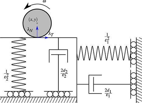
Throughout this paper, we consider an isotopic rigid sphere of uniform density that is free to rotate about an axis through its centre and is moving in a plane that is perpendicular to its axis of rotation. The coordinates of the centre of mass of the ball will be denoted by |$(x,y)$| and we denote its angular speed as |$\omega $|. It is assumed for simplicity that there is a single point of contact between the ball and a compliant surface. The contact force acting on the ball can be decomposed into the normal and tangential components, denoted by |$\lambda _N$| and |$\lambda _T$|, respectively. See Fig. 2 for an illustration.
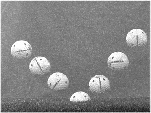
A combination of frames from a recorded high-speed video of a ball bounce (from left to right). Frames have been selected in irregular time steps for ease of view.
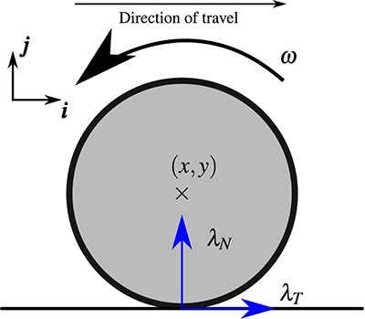
Setting of the notation used.
We shall consider different models for the viscoelastic compliance of the surface, starting from the simplest models of instantaneous impact with friction (Stronge, 2000), to those that allow for a finite time interval of contact from impact to lift off, under assumptions about the viscoelastic properties of the surface. To establish some notation, we shall choose an origin of co-ordinates so that at the moment of impact, the ball is at the origin, so that |$(x_0,y_0)=(0,0)$| and is travelling with initial horizontal velocity |$\dot{x}_0$| and vertical velocity |$\dot{y}_0<0$|. We shall henceforth choose a length scale such that the ball has unit radius |$R=1$|. The angle of incidence is defined as |$\phi = -\arctan (\dot{x}_0/\dot{y}_0),$| and denotes the angle away from the vertical axis. Similarly, the spin in the plane of motion at impact is denoted by |$\omega _0$|, which can either be positive (counter-clockwise rotation, or backspin) or negative (clockwise rotation, or topspin). This quantity will always be expressed in |$\mathrm{rad\,s}^{-1}$|.
2.1 Experimental observations
The main motivation for this paper is the recent set of experimental measurements obtained on golf ball bounce, the details of which are presented in the companion paper (Biber et al., 2022). Using a bespoke launcher, golf balls with a wide variety of incoming velocities and spins were launched at two different surfaces: an artificial turf and a well-maintained teeing turf. The results were captured using high-speed photography at frame rates of up to 10,000 frames per second. Figure 1 shows an example field of view. Automatic image processing enabled accurate measurement of time series of velocities and spin within the plane of the ball’s motion. In all cases it was found that the ball remained in contact with the surface for a finite amount of time, during which clear deformation of the ground could be seen, by noting that the position of the top of the ball fell and then rose. Nevertheless, for the range of impact velocities considered, there was little evidence of permanent plastic deformation of the surface. The range of initial conditions covered by the experimental campaign can be seen in Table 1, and a visual overview is presented in Fig. 3. The full data set is explained in detail in Biber et al. (2022); we just present here a few aspects, in Figs 4 and 5, of importance to the rest of this paper.
Range of initial conditions used in the experimental campaigns. For rescaling of data see the main text.
| Astroturf | Real turf | |||
|---|---|---|---|---|
| Dimensional range | Rescaled range | Dimensional range | Rescaled range | |
| |$\dot{x}_0$| | |$(1.53,\,38.6) \, [\text{m s}^{-1}]$| | |$(71.1,\,1810)$| | |$(0.0171,\,36.8) \, [\text{m s}^{-1}]$| | |$(0.801, \, 1720)$| |
| |$\dot{y}_0$| | |$(-36.4,\,-4.61) \, [\text{m s}^{-1}]$| | |$(-1710,\,-216)$| | |$(-33.0,\,-2.14) \, [\text{m s}^{-1}]$| | |$(-1550,\,-101)$| |
| |$\omega _0$| | |$(-4550,\, 1040) \, [\text{rpm}]$| | |$(-477,\,1090)$| | |$(-3880,\, 1090) \, [\text{rpm}]$| | |$(-407,\,1140)$| |
| |$\phi $| | |$(13.6^{\circ },\, 71.7^{\circ } )$| | |$(0.5^{\circ }, \, 73.6^{\circ } )$| | ||
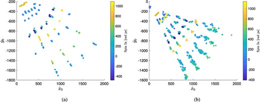
An overview of the span of the initial condition space. Note that the lengths are in units of ball radius. (a) Initial conditions obtained for the testing of artificial turf; (b) Initial conditions obtained for the teeing turf.
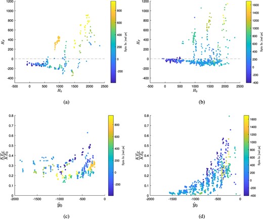
Scatter of the experimental results. Top panels: tangential velocity at lift off versus tangential velocity at first contact; (a) using artificial turf, (b) using fairway turf. The horizontal line represents zero tangential velocity at lift off. Bottom panel: change in kinetic energy as the normal component of initial velocity is varied (c) using artificial turf; (d) using fairway turf.
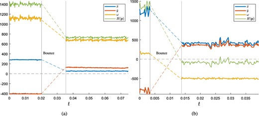
Two examples of raw time series data from the artificial turf data showing (rescaled) velocity vector |$(\dot{x}(t)$|, |$\dot{y}(t)$| and spin |$\omega (t)$| of the ball centre of mass, and tangential velocity |$H(t)$| of the contact point before and after a bounce. (a) A case with high positive |$H(t)$| at lift off. (b) A case of spin reversal where |$H(t)$| becomes negative negative at lift off.
Panels 4(a) and (b) show the relation between the incoming and outgoing relative tangential velocity |$H(t)$| between the contact point of the ball and the surface at the start and the end of the bounce. The results are presented using the notation of Section 4, where, in a rescaled length scale for which ball radius |$R=1$|, we write
We also use the notation |$H_0 = \dot{x}_0 + \omega _0$| to denote the tangential velocity component at the moment of impact and |$H_F = \dot{x}_F + \omega _F$| at the moment of lift off.
We observe that for both the synthetic and actual turf, the data in Fig. 4(a) and (b) fall roughly into two classes. For one class, the tangential velocity at lift off is large and positive. Further examination of the data reveal that these cases correspond to trajectories that land with a large amount of backspin (that is, a large positive |$\omega _0$|), slip throughout the bounce impact and lift off with a reduced amount of backspin. Another somewhat larger class of samples appear to lift off with small negative relative tangential velocity |$H_F$|. Analysis of the trajectories show that these trajectories typically enter with a small amount of backspin, no spin or topspin but lift off with a small amount of topspin. In particular, there is little evidence of balls lifting off rolling, that is, with the relative tangential velocity |$H_F=0$|.
Panels 4(c) and (d) present another aspect of the data, namely the dissipative nature of the bounce. Here we plot, for each data point, the ratio between total kinetic energy (from both linear and angular momentum) of the ball on landing, and the same quantity on lift-off. Note how highly dependent this effective ‘total energetic restitution coefficient’ is on the initial velocity and spin, with significant evidence of nonlinearity. These data suggest a physical process which is viscoelastic in that energy is dissipated, not just by friction, but by a rapid mechanical damping-like process in which energy is dissipated, presumably mostly through surface waves within the turf. Note how the nature of the dissipation varies between the two turf types, where the proportion of stored elastic energy for the fairway turf appears to tend to zero for high incoming normal velocities, whereas it approaches a finite value of about |$20\%$| for the artificial turf.
Examples of the raw time-series data for each of the two cases are illustrated in Fig. 5. Note that the rapid changes in velocity and spin during the bounce were not able to be reliably recorded, not least because the ball was not fully visible in that phase due to its partial immersion within the surface. For this reason, the precise time interval of contact was also not measured.
2.2 Instantaneous impact with friction
Let us first look at instantaneous bounce models, that is, where we assume a rigid ball bounces off a rigid surface subject to Coulomb friction, but with a discrete energy loss captured by a restitution coefficient. In the case of oblique impacts, a number of different approaches can be made to capture energy loss through a combination of coefficients of restitution and friction; see e.g. Brogliato (2018) and references therein.
Here we follow the approach used in Stronge (2000) where the impact is assumed to last an infinitesimal amount of time and the contact forces to be |$\delta $|-function-like distributions. An important part of the process is to model transitions between roll and slip during the infinitesimal impact. This can lead to subtle effects if the impacting body is slender (Nordmark et al., 2009). In the case of sphere, however, the implementation of an analogue to the single degree-of-freedom coefficient of restitution is straightforward and most methods lead to the same answer (Batlle, 1993). In particular here we assume, given the landing normal velocity |$\dot{y}_0$|, that lift-off is deemed to occur when the ball reaches a normal velocity |$\dot{y}_F = -r \, \dot{y}_0$|, where |$r$| is called a kinematic coefficient of restitution. For simplicity, we assume |$r$| is constant (although note the empirical studies Penner (2002); Roh & Lee (2010), and our data in Fig.4 which suggest golf turf may be better modelled by a velocity-dependent coefficient of restitution). We are interested in the dynamics of the point of contact, at which we can write the tangential and normal velocities as
so that
where the time variable |$t$| is, as yet, undefined, |$\boldsymbol{\lambda }$| is the vector of contact forces and |$m^{-1}$| can be thought of as the inverse of the mass matrix in the ‘coordinate system’ |$(v_T, v_N)$|.
Let us denote by the subscript |$0$| quantities evaluated at the ‘time’ that impact is initiated. To pass to an infinitesimal limit, we first introduce a small parameter |$0<\varepsilon \ll 1$|, and consider the short time during which the ball is in contact |$t-t_0= \varepsilon \tilde{t}$|. During that time we assume |$\varepsilon \boldsymbol{\lambda }, v_T, v_N = {\mathcal{O}}\left ( 1\right )$|, and denote |$\tilde{ \boldsymbol{\lambda }} = \varepsilon \boldsymbol{\lambda }$|, so that
We now follow the idea introduced by Stronge in Stronge (2000), where we replace our independent time variable by the new one, namely the normal impulse
which is a strictly increasing function of |$\tilde{t}$|. Dropping the tilde (for simplicity of notation) and ignoring terms |${\mathcal{O}}\left ( \varepsilon \right )$| we now have, with respect to the new independent variable,
which is independent of |$\varepsilon $|, and so we can pass to the limit |$\varepsilon \to 0$|.
During the slipping phase of the motion |$\lambda _T = - \mathrm{sign}\left ( v_T \right ) \mu \lambda _N $|, where |$\mu $| is the coefficient of friction. Substituting this into Equation (2.6) and rearranging the derivatives to eliminate |$n$| we have that during the slipping phase of the rigid bounce
Defining the tangential force during the roll needs a bit more care. We note that during the roll |$v_T = \dot{x} + \omega =0$| and thus it must also be true that |$\ddot{x} + \dot{\omega } = \lambda _T+\frac{5}{2} \lambda _T = \frac{7}{2} \lambda _T=0.$| This in turns requires |$\lambda _T=0$| during the roll, which implies that once the ball enters rolling, it may never leave it, and lifts off during the roll. Combined with Equation (2.6) we have for the rolling stage of the bounce
With these equations it is straightforward to work out conditions under which |$v_N$| and |$v_T$| vary, which can be expressed graphically using the method presented in Nordmark et al. (2009), see Fig. 6. In particular, we distinguish between three cases in the space of initial conditions |$(\dot{x}_0,\dot{y}_0,{\omega }_0)$|:
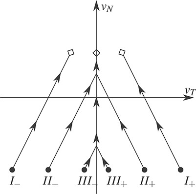
A graphic interpretation of changes in tangential and normal velocities during impact (Equations (2.7) and (2.8)). The start of the impact is denoted with solid black dot, and the end is denoted with a white rhombus. We differentiate between cases of slip throughout the impact (|$I_{\pm }$|) and slip followed by stick in the restitution (|$II_{\pm }$|) or compression (|$III_{\pm }$|) phase.
Case I: the ball will slip through the impact (case |$I_{\pm }$|) if
Case II: the ball will enter the roll in the restitution phase (case |$II_{\pm }$|) if
Case III: the ball will enter the roll in the compression phase (case |$III_{\pm }$|) if
Note that none of the cases allows the ball to enter slipping once it has begun to roll during the bounce. This contravenes what we saw in the experimental data. Specifically, if we consider balls entering bounce with |$v_T>0$| then, this theory allows lift-off from bounce to occur either in forward slip (|$v_T>0$|) or in roll |$(v_T=0)$|; there is no initial condition that leads to ‘spin reversal’ during bounce. Note though that this observation does not actually preclude a ‘backwards bounce’ because with high backspin a ball that has |$v_T=0$| would lift off with |$\dot{x}<0$|.
Note that the absence of spin reversal also occurs if we introduce a velocity-dependent kinematic coefficient of restitution, or introduce normal compliance into the theory, as in Hunt & Crossley (1975), so that the bounce occupies a short |${\mathcal{O}}\left ( \varepsilon \right )$| period of time, while keeping the Coulomb friction assumption in the tangential direction. For example, a straightforward calculation (in (Biber, 2023) for details) can be performed assuming a Kelvin–Voigt-like model of a spring and damper connected in parallel. Assuming the stiffness of the spring to be |$1/\varepsilon $| and the damping parameter of the dashpot to be |$d/\varepsilon $|, where |$d$| is a damping ratio, one obtains the same conclusion about the absence of spin reversal. In particular, in the limit |$\varepsilon \to 0$|, with |$d< \frac{1}{2}$| (to assure an underdamped solution), one recovers the rigid bounce theory, with the coefficient of restitution
More generally, it is clear that in order to observe spin reversal in a simple point-contact model, a more complex model of the mechanics in the tangential degree of freedom is required.
3. Linear viscoelastic model
Let us now consider a model where the ball remains rigid as before, but compliance in both horizontal and vertical directions can be observed. As depicted in Fig. 7, the viscoelastic behaviour is assumed to follow one of a spring and damper connected in parallel, known in the literature as the Kelvin–Voigt model, see e.g. Findley & Davis (2013). The dynamics between the normal and vertical directions is decoupled, and it is assumed that the ball is in contact with the surface at a single point only, where the normal and tangential forces again follow the Coulomb friction law. The equations of motion for such a system can be written in the rescaled form
A linear viscoelastic bounce mechanism based on the Kelvin–Voigt model
Here |$\hat{g} = g/R$| is the rescaled acceleration due to gravity, |$\varepsilon _{1,2}$| are the stiffness ratios in horizontal and vertical directions and |$d_{1,2}$| are the damping ratios in the respective directions. Note the scaling that |$\varepsilon _{1,2} \ll 1$| is consistent with a time scale in which the bounce take places over a rapid time scale, and passing to the limit |$\varepsilon _{1,2} \to 0$| will result in a rigid model with a horizontal and vertical coefficients of restitution (determined by the damping ratios |$d_{1,2}$|), provided that |$d_{1,2}<1$| so that the system is underdamped. In particular, we will assume |$d_2<1$|, which will ensure that a ball coming into contact with the ground with |$\dot{y}_0<0$| will lift-off at some later time with |$\dot{y}_F>0$|.
Specifically, we can readily compute that the ball will remain in contact with the compliant surface for as long as
and will lift off when |$\lambda _N=0$|
Returning to the physical motivation of golf-ball–turf interaction, in addition to the scaling that |$\varepsilon _{1,2} \ll 1$|, we shall additionally assume that |$\varepsilon _1 \ll \varepsilon _2$|. Such a scaling implies that there is far greater compliance in the normal direction than the tangential. That this is a natural assumption can be understood by briefly considering instead the motion that would occur if |$\varepsilon _1 = \varepsilon _2$|, so that the stiffness experience is isotropic. In that case, in the absence of spin or damping, and assuming |$\dot{y}_0<0$|, a ball with inbound angle |$\phi = -\arctan (\dot{x} {/} \dot{y})$| (from the vertical) would move along a straight line in the |$(x,y)$|-plane and would lift off with angle |$\phi +\pi $|. This is not how turf behaves. Instead, observational data suggest that such a ball would lift with outbound angle close to |${\pi }-\phi $|.
With such scaling, it is useful to introduce a new time rescaling
and a dimensionless parameter
The equations of motion can now be written in the rescaled form as
where |$X(\tau ) = x(t)$|, |$Y(\tau ) = y(t)$|, |$\varOmega (\tau ) = \omega (\tau )$|, |$\varLambda _T=\varepsilon _2^{-2} \lambda _T$|, and a prime represents differentiation with respect to |$\tau $|. We also define |$\varLambda _N = \varepsilon _2^{-2}\lambda _N,$| that is,
The Coulomb friction law (in the new variables) dictates that for |$\lvert \varLambda _T \rvert = \mu \varLambda _N$| the ball slips on the surface. However, greater care is needed for the rolling motion, that is when |$\lvert \varLambda _T \rvert{<} \mu \varLambda _N$|.
3.1 Defining rolling; a Filippov formulation
To consider what happens during rolling, it is useful to model the system as a Filippov System (Filippov, 1988; Bernardo et al., 2008; Jeffrey, 2018). That is, with |$\varLambda _T$| well defined for the cases of slip, we note that the equations (3.5) can be written in the form
where |$\boldsymbol{p}$| is the vector of state variables. Specifically, we have
and the smooth function
In 1988 Filippov (Filippov, 1988) proposed a consistent method of defining dynamics along the surface of discontinuity |$\{H(\boldsymbol{p})=0\}$| in which a new vector field is introduced
where |$\alpha \in [0,1]$|. That is, the vector field along the discontinuity surface is the unique convex linear combination of the two neighbouring vector fields, such that the resulting vector lies along the discontinuity. The vector field |$F_s$| in our system would define rolling, but confusingly, in deference to control applications, in Filippov systems |$F_s$| is termed the sliding vector field.
A ‘sliding’ trajectory is allowed to leave the surface of discontinuity when either |$\alpha = 0$| (therefore leaving into the region |$H(\boldsymbol{p})>0$| where vector field |$F_1$| applies) or when |$\alpha =1$| (where |$F_2$| applies). At the same time, |$\alpha $| can be explicitly calculated during the sliding motion by making that the assumption that the vector field must be orthogonal to |$\nabla H$|. Thus, we have
3.2 Analysis of roll, slip and lift-off transitions
Having now defined the dynamics fully to be
with |$F_S$| specified in Equation (3.10), we can consider different cases of dynamics during the bounce. We represent possible geometries in Fig. 9. In the figure we note that a ball can either slip throughout the bounce (either forward slip with |$H(\boldsymbol{p})>0$| or negative slip with |$H(\boldsymbol{p})<0$|) or can at some time |$t$| begin to roll (that is, the dynamics evolves along the discontinuity set where |$H(\boldsymbol{p}) =0$|).
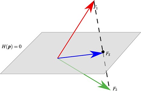
Definition of the sliding dynamics—the discontinuity surface is denoted here with a plane (|$H(\boldsymbol{p}) = 0$|); the dynamics according to the two vector fields |$F_1$| and |$F_2$| are denoted with the red and green arrows (above and below the discontinuity surface). Their convex linear combination lies along the dashed line, and we chose the unique solution that also aligns with the sliding surface.
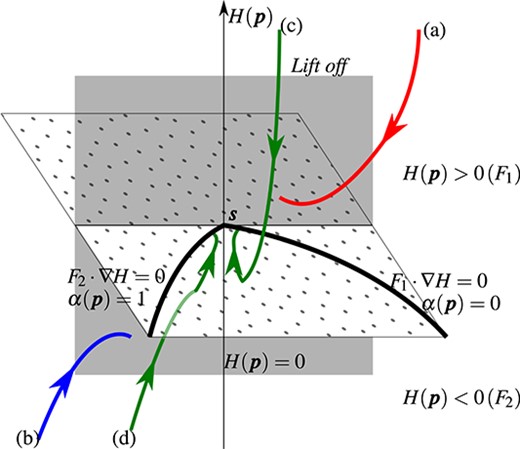
Possible trajectories during the generic viscoelastic bounce (in reduced geometry). The grey plane represents the lift-off condition, the dotted plane is the codimension-one discontinuity and the solid black curves represent surfaces where |$F_1 \cdot \nabla = 0$| and |$F_2\cdot \nabla H = 0$|, which corresponds to the surfaces where a trajectory leaves the surface of discontinuity and enters either |$F_1$| or |$F_2$|, respectively. Point |$\boldsymbol{s}$| is an intersection of the two switching surfaces (known as a two-fold bifurcation point (Jeffrey, 2017)) and lies on the lift off plane as well. Red trajectory (a): The ball goes through the bounce with positive slip only (|$H(\boldsymbol{p})>0$|). The bounce is terminated by the intersection with the grey plane, which represents the lift-off condition. Blue trajectory (b): The ball goes through the bounce with negative slip only (|$H(\boldsymbol{p})<0$|). The bounce is terminated by the intersection with the grey plane, which represents the lift-off condition. Green trajectories (c–d): The ball enters the bounce with positive or negative slip, respectively, and eventually reaches the system discontinuity by entering roll (|$H(\boldsymbol{p}) =0$|). The bounce dynamics continue along the surface of discontinuity and are to be determined in the next sections.
Let us now direct our attention to the latter of the presented cases, that is, when the ball is rolling and in particular, we shall study how exiting such state is possible. As discussed before, exiting will be dependent on the value of the function |$\alpha (\boldsymbol{p})$|, which for our system is explicitly calculated to be
We now analyse the transitions between rolling and slipping.
Suppose, for definiteness, that a trajectory along the discontinuity surface |$H(\boldsymbol{p}) =0$| reaches a point |$\boldsymbol{p}_1$|, where |$F_1(\boldsymbol{p}_1) \cdot \nabla H = 0$|, which means that the sliding field definition is equal to the vector field |$F_1$| at this point. Moreover, as dictated by (3.11), the trajectory should leave the surface into the half-space |$H(\boldsymbol{p}_1)>0$|. Such a trajectory leaving the discontinuity surface must be tangent to |$H(\boldsymbol{p}_1) = 0$|, therefore we have
Notice that the term |$2d_2 Y^{\prime} + Y + \varepsilon _2^2 {\hat{g}} $| is in fact the |$-\varLambda _N$|, given by (3.6) and thus remain negative throughout the bounce. On the other hand, in order to balance the first two terms on the right-hand side of (3.14), at |$\boldsymbol{p}_1$| we must have that |$\varLambda _N = {\mathcal{O}}\left ( \eta \right ) \ll 1$|.
Given this information, let us now consider the possible signs of the state variables at |$\boldsymbol{p}_1$|. The bounce is initiated at |$Y=0$| and |$Y\leq 0$| throughout the bounce. Suppose that at |$Y^{\prime}<0$| at |$\boldsymbol{p}_1$|, so that we are in the downwards (compression) phase of the bounce. Then since |$\varLambda _N = {\mathcal{O}}\left ( \eta \right )$| and |$Y<0$| it must follow that both |$Y, Y^{\prime} = {\mathcal{O}}\left ( \eta \right )$| at |$\boldsymbol{p}_1$|. |$Y$| being small means we must be close to the time of initiation of bounce. However, initially |$Y^{\prime}(0) = {\mathcal{O}}\left ( 1\right )$| which gives a contradiction. Thus, we must have that |$Y^{\prime}>0$| at |$\boldsymbol{p}_1$|. That is, the transition from roll into slip can only happen during the upward (restitution) phase of the bounce.
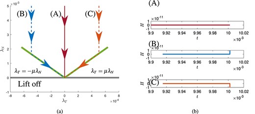
Numerical results for the system (3.5) for |$\mu =0.3$|, with three different initial conditions; (a) projected onto the friction cone|$(\lambda _T,\lambda _N)$| and as slip velocity |$H$| as a function of time. See the text for details.
Next, let is compute the second directional derivative at such a point |$\boldsymbol{p}_1$|. We obtain
Now, the above argument shows that both of the terms on the right-hand side of (3.15) are positive. Thus |$\left ( F_1 (\boldsymbol{p}_1) \cdot \nabla \right )^2 H>0$|, which confirms that the ball will leave the rolling region consistently into the |$F_1$| region.
We can similarly analyse we the case where the ball transitions from rolling to slipping via the sliding flow becoming tangent to the vector field |$F_2$| at some point |$\boldsymbol{p}=\boldsymbol{p}_2$|. We now have
As before, we see that such point can only occur if |$\varLambda _N={\mathcal{O}}\left ( \eta \right )$|. A similar argument shows that |$Y^{\prime}>0$| at any such point |$\boldsymbol{p}_2$|. The argument then follows as before. The second directional derivative at the switching point will thus be negative, once again confirming consistency of Filippov’s theory.
The key question for final consideration is whether the ball can lift off (that is, reach the termination point of bounce) while rolling. For that to be the case, we would need |$\varLambda _N=0$| as the lift off condition, but thus also |$\varLambda _T=0$|, which can be thought of |$F_s$| being tangent to |$F_1$| and |$F_2$| simultaneously. Considering the form of the function |$\alpha (\boldsymbol{p})$| we would have that precisely at lift off we must simultaneously satisfy the two conditions
which imposes an additional constraint on the initial-value problem. Thus there will be at most a codimension-one surface in the space of initial conditions for which both conditions can be simultaneously satisfied and lift off with rolling would occur with probability zero. However, to make this statement more precise requires a proper analysis of the singularity where |$F_s$| is simultaneously tangent to |$F_1$| and |$F_2$|, because it is possible that the point satisfying (3.17) could be an attractor for sliding initial conditions. Such an analysis forms the subject of the next section.
Briefly though, Fig. 10 shows a numerical verification that lift-off with roll seems to not be an attractor in this case. Here trajectory (A) with initial conditions |$\boldsymbol{p}_0 = [0.3543,\, -0.1603128, \,-0.1608, \, 3.4739, 0.1603128]^{\intercal }$| is the trajectory which leaves the bounce within the friction cone, thus rolling. Initial conditions of trajectory (A) is perturbed slightly and gives rise to trajectories (B) and (C), which lift off on the boundary of the slipping cone, therefore slipping. (b) Tangential velocities of each of the trajectories. Note how trajectories (B) and (C) enter slipping motion (non-zero tangential velocity |$H$|) shortly before lift-off.
Thus we have found precisely the opposite conclusion from the rigid impact model in Section 2.2, namely that an introduction of even minimal compliance in the normal direction causes the ball to always lift off slipping. That is, despite a transition to roll during the bounce, with probability zero does the ball lift off rolling. This conclusion appears to be consistent with the experimental data, but it would be useful to check whether it is an artefact of the specific linear Kelvin–Voigt model we have chosen.
4. A generalized viscoelastic model
To test the generality of our findings to refinements in the surface model, we now consider a generalization of the model from the previous section, which would allows us to capture the more general nonlinearity and velocity-dependence seen in the data in Fig. 4(c) and (d). Specially, we suppose more general nonlinear equations of motion of the form
where |$u,\, z,\, d,\, k$| are general, possibly nonlinear, functions, |$g$| is the acceleration due to gravity and all other variables have the same meaning as before. Note this model allows for nonlinear, and velocity-dependent stiffness and damping coefficients, as well dependence of the tangential mechanics on depth, spin and normal velocity. We will however impose some asymptotic constraints on the functions |$u,\, z,\, d$| and |$k$| in the course of our theory (see equations 4.34.7 below).
Under our assumption of a point of contact, we assume that the frictional contact between the ball and the surface can be modelled according to the Coulomb friction law, that is,
during slipping and
when the ball is rolling (sticking), where |$\mu $| is the coefficient of friction.
The ball will remain in contact with the surface until normal forces due to the mechanism are balanced by those due to gravity, that is, when
We will refer to (4.2) as the lift-off condition; the horizontal and vertical velocities at this instance will be denoted by |$\dot{x}_F$| and |$\dot{y}_F$|, respectively, and the lift-off spin denoted by |$\omega _F$|.
One can think of the form of (4.1) as a Kelvin–Voigt-like model, where springs and dampers, connected in parallel, dictate the behaviour of the sphere during the bounce in the vertical and horizontal direction independently. The major difference between the classical Kelvin–Voigt model and the one used here is that the springs and dampers are allowed to be nonlinear and to feature coupling between normal and tangential degrees of freedom. An illustration of this set-up can be seen in Fig. 11.
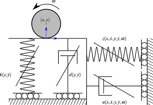
A generalized viscoelastic point contact model.
We impose certain conditions on our functions |$u,z,d,k$| suggested by physical intuition and what was observed in our experimental data. First, we require the stiffness and damping in both vertical and horizontal directions to increase as the ball moves further into the bouncing surface, that is, those values should increase as the vertical position |$y$| decreases:
The motivation for this is that in reality, point contact is an approximation to a Hertzian-like contact in which the true area of contact increases with depth |$-y$|. Also, we assume that the range of normal velocities we consider means the ball does not reach the point half-immersion, where the contact area reaches a maximum with respect to depth.
In a similar fashion, we require that the normal force acting on the body increases with depth
Given that the ball is landing with |$\dot{x}_0>0$|, in the horizontal direction we will require that the stiffness increases when the ball is moving to the right, and decreases when the ball reverses (moves to the left):
Our analysis is motivated by the case of a rapid ball bounce, which we suppose to take |${\mathcal{O}}\left ( \varepsilon \right )$| amount of time, where |$\varepsilon \ll 1$|. We thus introduce a re-scaling of time
and with it, we denote state variables in the new variable as |${X} (\tau ) = x(t),\, {Y}(\tau ) = y(t),\, \varOmega (\tau ) = \omega (t)$|. To ensure the appropriate balance of terms in (4.1) we now require
where |$^{\prime} = \frac{\mathrm{d}}{\mathrm{d} \tau }$| denotes the derivative with respect to the new time variable |$\tau $|, and |$\kappa ({Y}, {Y}^{\prime}), \delta ({Y}, {Y}^{\prime}) \sim{\mathcal{O}}\left ( 1\right )$| are general functions.
At the same time, we anticipate a much greater stiffness in the horizontal direction than in the vertical section. One can think of this requirement as avoiding the case of a ‘jelly-like’ surface, where the symmetry in vertical and horizontal direction would cause an outbound trajectory, in the absence of spin, to be the time-reverse of the incoming trajectory, irrespective of the angle of incidence with the surface. We will thus introduce a distinguished scaling so that the damping and stiffness function in the horizontal directions to be
Our final requirement on the rescaled function |$\kappa $|, |$\zeta $|, |$\delta $| and |$\upsilon $| is that their (partial) derivatives with respect to the state variables be at most of |$\mathcal{O}(1)$|. That is, we do not expect abrupt changes in the material constants with displacement or velocity. That is, taking |$q$| to be any of the state variables |${X}, {X}^{\prime}, {Y}, {Y}^{\prime}, \varOmega $| we have that
Following the rescaling and the introduction of new functions, the resulting dynamical system for modelling the bounce becomes
where |$\varLambda _T = \varepsilon ^2 \lambda _T $|.
The conditions introduced in (4.3), (4.4) and (4.5) can now be written in the form
and
The Coulomb friction law once again defines our dynamics for the slipping motion, where
where
and |$\boldsymbol{p}$| is once again the five-dimensional vector of dynamical coordinates defined by (3.8). Compared with the simple analysis in Section 3 additional consideration is needed for the rolling motion, when |$H(\boldsymbol{p}) = {X}^{\prime} + \varOmega =0.$| Precise study of the onset and loss of rolling motion and their implication for the overall dynamics will be our main interest in what follows.
We note, finally, that our formulation allows to capture various forms of nonlinear viscoelastic deformation models that have been proposed in the literature, see e.g. Hunt & Crossley (1975); Hoffmann & Gaul (2003). However, our aim here is not to fit coefficients of a particular model, but to show that for this more general class of models, the conclusions of the previous section remain valid; namely that lift-off in a state of rolling represents a codimension-one transition between pure slip and slip reversal.
4.1 The two-fold singularity
Let us consider again the possibility of lift off while rolling. Recall that at lift off |$\varLambda _N = 0$| and as such the definition of friction dictates that we must also have |$\varLambda _T=0$|. At the same time, to agree with the formulation as a Filippov System, the lift-off point must coincide with the lower-dimensional spaces where |$\alpha (\boldsymbol{p}) = 0$| and |$\alpha (\boldsymbol{p}) = 1$|. Such point is denoted as |$\boldsymbol{s}$| in Fig. 9.
The point where the two switching surfaces (|$\alpha = 0$| and |$\alpha =1$|) coincide is known in the literature as the two-fold singularity (Jeffrey, 2017). It is now of our interest to determine whether such point is attracting or not. Indeed, an attracting two-fold singularity (which we will from now on denote as point |$\boldsymbol{s}$|), will mean that rolling trajectories will tend towards it, therefore reaching lift off with |$H(\boldsymbol{p})=0$|. Alternatively, if |$\boldsymbol{s}$| is not attracting, there will only be a finite number of lower-dimensional trajectories tending to |$\boldsymbol{s}$|.
A full unfolding of two-fold singularity can be found in Jeffrey (2018) with the formal results following from Theorems 6.1 and 6.2 in the aforementioned book. We look at the case of our interest only in this paper.
Let us consider an |$n$|-dimensional discontinuous system
where |$H(\boldsymbol{p}) = 0$| is the discontinuous surface, along which |$\boldsymbol{p}^{\prime} = F_s(\boldsymbol{p}) = (1 - \alpha (\boldsymbol{p}))\, F_1(\boldsymbol{p}) + \alpha (\boldsymbol{p}) \, F_2(\boldsymbol{p})$|, with |$\alpha $| defined by Equation (3.11) as before.
Suppose the system posses two switching surfaces |$\alpha (\boldsymbol{p}) = 0$| (equivalent with |$(F_1 \cdot \nabla ) H(\boldsymbol{p})$|) and |$\alpha (\boldsymbol{p}) = 1$| (equivalent with |$(F_2 \cdot \nabla )H(\boldsymbol{p})$|) which intersect at a point |$\boldsymbol{s}$|.
We define new coordinates:
where
We note that |$z_1=0$| is precisely the discontinuity surface of (4.15) with |$z_2=0$| being equivalent to the switching surface |$\alpha =0$| and |$z_3$| being equivalent to |$\alpha =1$|. Thus, the two-fold singularity is precisely the |$n-3$| dimensional manifold |$\{(\boldsymbol{z}=z_1, \dots , z_n) \,:\, z_1 = z_2 = z_3 = 0\}$|, with |$z_{4},\dots , z_n$| defined to be any |$n-3$| dimensional coordinates orthogonal to |$z_1, z_2$| and |$z_3$|.
In deriving the normal form of the dynamics we apply a time rescaling |$t \mapsto \varphi t$| when |$z_2<$| and |$t \mapsto t / \varphi $| when |$z_2>0$|. Since |$\varphi>0$| the phase portrait remains unchanged under this transformation.
With details and series expansions presented in the original source, one finds that in the neighbourhood of the two-fold singularity, under the transformations outlined before, the flow becomes
where
and
As discussed in Jeffrey (2017) the quantities |$\nu _{1,2}$| characterize the local curvature of the flow, with |$\nu _1 \nu _2$| quantifying the jump in the vector field |$F_{1,2}$| and the singularity.
With the new variables, along the discontinuity surface |$z_1 = 0$| we define (as before)
where |$\alpha $| is solved so that |$\dot{z}_1=z_1 = 0 $|. To the leading order the dynamics in (4.20) are independent of |$z_{4,\dots ,n}$|. Therefore, the dynamics in |$z_2$| and |$z_3$| can be separated and, with |$\alpha $| evaluated explicitly, we have the two-dimensional system
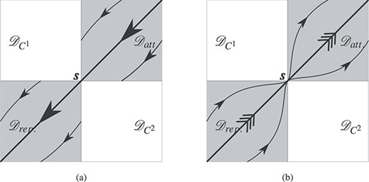
The two switching surfaces (or folds) |$z_2$| and |$z_3$| will divide the vector field along the discontinuity |$z_1=0$| into four regions
With such definition, the vector field outside of the discontinuity |$z_1=0$| is directed into |${\mathcal{D}}_{att.}$|, away from |${\mathcal{D}}_{rep.}$| and crosses |${\mathcal{D}}_{C^{ 1 }}$| in the direction of increasing |$z_1$|, and crosses |${\mathcal{D}}_{C^{ 2 }}$| in the direction of decreasing |$z_1$|.
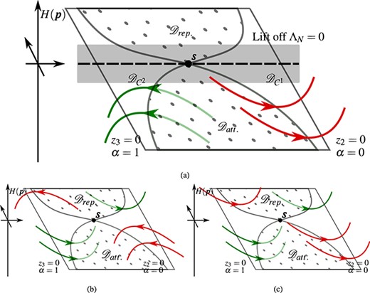
Classification of two-fold singularities, depending on the flow outside of the discontinuity surface. (a) Visible two-fold (interpreted for the case of a ball bounce, with the lift-off surface indicated). Here, the red trajectories correspond to flow with |$H>0$| and the green trajectories with |$H<0$|. (b,c) Adaptations to the above figure to deal with the (b) invisible two-fold and (c) the visible-invisible two-fold. Figure redrawn based on images in Jeffrey (2017).
According to Jeffrey (2018), three types of two-fold singularity can be distinguished based on the nature of the flow outside of the discontinuity surface, specifically the nature of the grazing tangencies at the sliding region; see Fig. 12. Each of these cases are analysed in detail; here we analyse only the case that is relevant to the ball-bounce problem, namely the visible case.
4.2 Visible two-fold singularity
When |$\sigma _1>0 > \sigma _2$| then |$\boldsymbol{s}$| is the intersection of visible folds, and we call such point a visible two-fold. Trajectories away from the discontinuity are presented in Fig. 12a. In this case (4.21) becomes
Understanding the nature of the fixed point |$(0,0)$| is a straightforward, albeit laborious, exercise in algebra. Detailed derivation can be found in (Jeffrey, 2018, chapter 13.4), we give the simple summary here.
The linearized system (4.23) will yield two eigenvalues |$\gamma _+$| and |$\gamma _-$|. For |$\nu _{1,2}>0$| and |$\nu _1 \nu _2>1$| we have that the two eigenvalues are such that |$0< \gamma _- < \gamma _+$| and the weak eigendirection lies along eigenvector |$\boldsymbol{\gamma }_-$| (corresponding to the eigenvalue |$\gamma _-$|). The flow will therefore generate a node, with the flow outwards from the singularity |$\boldsymbol{s}$| and into the attracting region |${\mathcal{D}}_{att.}$|. The phase portrait for that is shown in Fig. 13b.
Phase portraits for the visible two-fold singularity. (a) Case where |$\nu _1 \nu _2<1$| or when |$\nu _{1,2}<0$| and |$\nu _1 \nu _2> 1$|. (b) Case where ν1,2 > 0 and ν1ν2 > 1. Reproduced from Jeffrey (2017).
For |$\nu _1 \, \nu _2 <1$| we have that |$\gamma _-<0<\gamma _+$| and the inward eigendirection |$\boldsymbol{\gamma }_-$| lies in the regions of discontinuity |${\mathcal{D}}_{att.}$| and |${\mathcal{D}}_{rep.}$|. Only along the direction of |$\boldsymbol{\gamma }_-$| we have a single trajectory reaching |$\boldsymbol{s}$| from |${\mathcal{D}}_{att.}$| and all remaining trajectories will leave through the folds. The respective phase portrait is shown in Fig. 13a.
When |$\nu _{1,2}<0$| and |$\nu _1 \, \nu _2>1$| we find that the eigenvalues are such that |$\gamma _-<\gamma _+<0$| and again only a single trajectory along |$\boldsymbol{\gamma }_-$| passes through |${\mathcal{D}}_{att.}$| to |${\mathcal{D}}_{rep.}$| through |$\boldsymbol{s}$|, and again we obtain the phase portrait from Fig. 13a.
To proceed we therefore need to compute the normal form for the problem at hand and determine the signs of the quantities |$\nu _1$| and |$\nu _2$|. Referring back to Fig. 9 we see that reaching |$\alpha = 0$| (and thus entering |$H(\boldsymbol{p})>0$|), while being tangential to the flow in |$F_1$|, the trajectory is also at its minimum with respect to |$H(\boldsymbol{p})$|. A direct calculation shows that at |$\boldsymbol{s}$| (and thus also in the neighbourhood of |$\boldsymbol{s}$|):
where we have used that |$\varLambda _N(\boldsymbol{s}) = 0$| together with the constraint on the size of the derivatives (4.9). Noting that |$\boldsymbol{s}$| can only be reached in the restitution phase (i.e. when |${Y}^{\prime}>0$|) we see that |$\left (\nabla \cdot F_1\right )^2 H(\boldsymbol{s})>0$|, confirming thus that a trajectory leaving the rolling surface |$H=0$| through the switching region |$\alpha =0$| will indeed enter the |$F_1$| vector field as expected. A similar direct calculation shows that
which in turns confirms a consistent behaviour when leaving the rolling surface |$H=0$| through the switching surface |$\alpha =1$|.
Recalling that the classification of the two-fold singularity depends on the quantities |$\sigma _{1,2}$| (as defined by Equation (4.18)) from Equations (4.24) and (4.25), we find that
We thus have |$\sigma _1>0>\sigma _2$|, which indeed confirms from (4.1) that this is a visible two-fold singularity.
Let us now determine The signs of |$\nu _{1,2}$|. From (4.19) we have that
where |$D = \sqrt{\left |\left (F_1 \cdot \nabla \right )^2 H(\boldsymbol{p}) \cdot \left (F_2 \cdot \nabla \right )^2 H (\boldsymbol{p})\right |}>0$| by definition. By our assumption (4.12) we have immediately |$\nu _{1,2} < 0$|, and thus we obtain a phase portrait shown in Fig. 13a. This is the case where |$\boldsymbol{s}$| is a non-attracting point, with only a single trajectory passing through it within the normal form.
Interpreting our result with respect to the ball bounce, we note that the ball that enters rolling during the bounce (governed by the aforementioned conditions) can only leave with a roll along a codimension-one manifold within the space of initial conditions. Thus, with probability 1, the ball must leave slipping.
4.3 Rigid bounce revisited
Let us briefly return to the case of the rigid bounce studied in Section 2.2. We concluded the studies in that section with a result, where a ball that entered rolling during the bounce could no longer enter the slip. One could think that this contradicts our main result here—but the case is more subtle than that.
The rigid bounce is a limiting case of the model studied in this paper, where the tangential compliance tends to zero; |$\varepsilon \rightarrow 0$|. This, in turn, means that the quantity |$\nu _1\,\nu _2= 1$|, and hence the normal form of the visible two-fold singularity given by (4.23) is based on a singular matrix. Classification is thus more convoluted than that for the general case, but has already been studied in detail in (Jeffrey, 2018, chapter 13) and is known as the diabolo bifurcation.
Rather than studying the singularity for that case in detail, one can notice interesting geometries about that case. Since the lack of tangential compliance affects the tangential force during the roll, the Filippov formulation should lead to an ‘equal’ contribution from the two vector fields |$F_1$| and |$F_2$|. Explicit calculation of the function |$\alpha (\boldsymbol{p})$| as given by Equation (3.11) shows |$\alpha =1/2$| throughout the roll, and thus |$F_s(\boldsymbol{p}) = \left (F_1(\boldsymbol{p}) + F_2 (\boldsymbol{p})\right )/2$|.
The geometry on the friction cone is thus quite simple—all trajectories that enter the discontinuity (roll) region land precisely on the attracting trajectory that leads to a lift off with roll. In other words, that attracting trajectory is the only trajectory allowed in the rolling region for the case of the rigid bounce under Filippov’s formulation.
5. Conclusion
Inspired by empirical observations on the experimental data from (Biber et al., 2022), we used Filippov theory to analyse ball bounce within generalized point contact models that have both normal and tangential compliance. Under physically realistic scaling laws, we show that a rigid spinning sphere will typically lift off with some non-zero relative tangential velocity. The case of rolling lift off forms the boundary case between forward and backward slipping cases, and therefore should not be observed in practice. This is contrary to a much more well-studied and well-understood problem of a rigid ball bouncing off a rigid surface. We have identified the underlying principle of the slip and roll transition, which has not been considered in detail before, and a careful understanding of that will be paramount to future modelling.
We are now in possession of what is thought to be the largest data set on the given problem; however fitting the models to the data remains to be an issue. Indeed, the focus of our analysis, that is, the discontinuity, makes it difficult to find a structured and widely applicable ways of fitting the models to the data.
With appropriate measurements, it is easy to decide whether the observed bounce trajectory entered roll at some point or not. One of the most challenging tasks of the modelling will thus be to solve that problem in the initial condition space. That is, given the data, future work will be aimed at identifying the lower-dimensional divide of the space which will identify the initial condition that will lead to the bounce with slip only and those that will enter gripping at some point.
The aim of identifying such key features is to allow for more precise modelling of the compliant surface, in particular in the game of golf. A particular basis of nonlinear functions can be selected and thus fitted with appropriate parameters using the data available. Avoiding high-dimensional problems or finite element solutions remains an open problem.
A part of the problem at hand is identifying parameters together with their physical meaning and the ways to measure them. The golf industry currently tends to quantify the ground’s firmness and stiffness using either USGA TruFirm (Turf-thumper) device or the Clegg Hammer—the measurements performed by these are centred around measuring the deceleration of a free-falling object. There is some evidence, however, showing that behaviour of a ball on two turfs with similar measurements can be significantly different, thus suggesting that important properties are not captured by either of the tools (Baker et al., 2005).
Some immediate extensions of the problem considered are evident and present an interesting challenge. One could possibly resolve more complex contacts such as Hertzian using the current formulation, thereby extending this study to the models of elastic half spaces (Haake, 1989; Barber, 2018). A further idea to explore would also involve a side spin, that is, a spin outside of the plane of travel of the ball. This could present a generalization of the problem to many other disciplines, applicable to a further ball-sports and also a wider set of impact-problems in general. Both of the aforementioned extensions would require the extension of modelling friction in 3D, a problem that presents a far greater order of complexity and requires a more considerate approach, whether through the extension of the current models or the regularization of such in higher dimensions—see e.g. (Antali & Stepan, 2019; Cheesman et al., 2022).
Acknowledgements
This work is being partially funded by the EPSRC and by the industrial partner R & A Rules Ltd., who have also actively participated and facilitated this research. We thank the industrial partner for allowing us to run the experimental campaign using their research facilities, and particularly acknowledge helpful advice from Kristian Jones, Andrew Johnson and Steve Otto.
Further thanks go to Mike Jeffrey (University of Bristol) for useful discussions on non-smooth dynamics. We also thank two anonymous referees for bringing additional references to our attention.
Funding
This work was funded by EPSRC Doctoral Training Award at the University of Bristol and R&A Rules limited.
Conflict of interest
The work was partially funded by R&A Rules Limited who governs the sport of gold worldwide, outside of the United States and Mexico.
References
