Modelling alternating current effects in a submerged arc furnace

Abstract

Modelling the production of silicon in a submerged arc furnace (SAF) requires accounting for the wide range of timescales of the different physical and chemical processes: the electric current which is used to heat the furnace varies over a timescale of around $10^{- 2}$ s, whereas the flow and chemical consumption of the raw materials in the furnace occurs over several hours. Models for the silicon furnace generally either include only the fast-timescale, or only the slow-timescale processes. In a prior work, we developed a model incorporating effects on both the fast and slow timescales, and used a multiple-timescales analysis to homogenise the fast variations, deriving an averaged model for the slow evolution of the raw materials. For simplicity, in the previous work we focussed on the electrical behaviour around the base of a single electrode, and prescribed the current in this electrode to be sinusoidal, with given amplitude. In this paper, we extend our previous analysis to include the full electrical system, modelled using an equivalent circuit system. In this way, we demonstrate how the two furnace-modelling approaches (on the fast and slow timescales) may be combined in a computationally efficient way. Our previously derived model for the arc resistance is based on the assumption that the dominant heat loss from the arc is by radiation (we will refer to this as the radiation model). Alternative arc models include the empirical Cassie and Mayr models, which are commonly used in the SAF literature. We compare these various arc models, explore the dependence of the solution of our model on the model parameters and compare our solutions with measurements from an operational silicon furnace. In particular, we show that only the radiation arc model has a rising current-voltage characteristic at high currents. Simulations of the model show that there is an upper limit on the length of the furnace arc, above which all the current bypasses the arc and flows through the surrounding material.

submerged arc furnace, equivalent circuit model, heat transfer, electric arc, periodic solutions of non-linear systems, non-linear dynamics

Issue Section:

Articles

1. Introduction

Silicon is produced industrially by reducing quartz (containing SiO $_{2}$ ⁠) with carbon in a submerged arc furnace (SAF), which is heated by an alternating electric current. The current is provided to the furnace via three electrodes, and passes through the material bed either by conducting through the partially reacted materials, known as the charge material, or as an electric arc, a gas discharge which forms in gas-filled craters at the base of each electrode. A diagram of a silicon furnace, showing two of the three electrodes and the crater beneath each one, is given in Fig. 1.

One major difficulty of modelling SAFs is the disparity in the timescales of the different processes in the furnace (Andresen, 1995). The applied alternating current (AC) has a frequency of around $50$ Hz, and so variations of the electrical system occur on a timescale on the order of $10^{- 2}$ s. The chemical consumption and flow of the charge material in the furnace is a much slower process, with a timescale of hours (Luckins et al., 2021). The interactions between these different-timescale processes are important in the production of silicon. For instance, the amount of heat transferred from the electric arc to the surrounding charge material varies periodically over the AC timescale, and this is the main source of heat for the charge material. However, the timescale of the heat transfer, melting, and reactions within the charge material is much slower. Conversely, the electrical conductivity or resistance of the charge material (which depends on its composition and temperature) varies slowly, but the resistance of the charge material is important when studying the distribution of current in the furnace. In turn, this affects the heat dissipated by the electric arc, and thus the slow- and fast-timescale processes are fully coupled. In order to retain numerical tractability, the majority of furnace models only include effects on one of these timescales and not both.

For instance, the fast-timescale electrical variations in the furnace may be modelled by an equivalent circuit (EC) approach, in which all the regions of the furnace are modelled as elements in an electric circuit, and equations relating the currents, voltages, resistances and inductances of the circuit elements are derived using Kirchhoff’s electric circuit laws. An EC model of this type has been developed by Valderhaug (1992) for the three-phase electrical system of a silicon SAF; the model we will use in this paper is based on that of Valderhaug (1992).

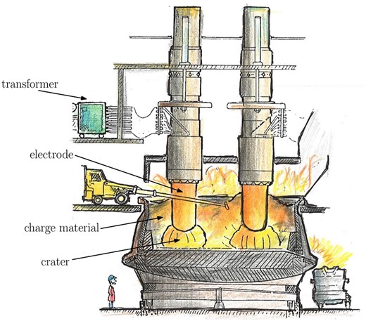
Fig. 1.

Drawing of an SAF for silicon production, adapted from Hannesson (2016), showing the main regions of the furnace, two of the three electrodes and the connection to the external electrical system.

Open in new tab Download slide

An important element of EC models for SAFs is the sub-model for the resistance of the electric arcs. Each arc consists of a region of hot gas ionised to a plasma, so that it is electrically conductive. The Ohmic heating due to the high current density and resistance in the arc generates heat which is transferred primarily by radiation to the surrounding material, providing much of the energy for the chemical reactions in the furnace. The electrical, thermal and fluid flow in an arc are closely coupled, and magnetohydrodynamic (MHD) models have been used to simulate an SAF arc in isolation (Andresen, 1995; Saevarsdóttir, 2002). However, this MHD approach is too complicated to include in the EC models. In Valderhaug (1992), the arc resistance is related to the voltage applied across the arc using a Cassie arc model (Cassie, 1939). This is one of several empirical models for arc resistance. Others, including those of Mayr (1943a,b), Schwarz (1971), and hybrid versions, are discussed in Gustavsson (2004), Parizad et al. (2009) and Yuan et al. (2013). These models have all been developed for the electric arcs in circuit breakers, to understand short-circuiting phenomena. Nevertheless, the models are widely used for the arcs in SAFs and open-air electric arc furnaces (Awagan & Thosar, 2016; Barker et al., 2007; Bhonsle & Kelkar, 2014; Bowman & Krüger, 2009; Golestani & Samet, 2016; Logar et al., 2011). Other semi-empirical arc models such as the ‘channel arc models’ (CAMs) have been developed that are designed to take into account additional heating and heat loss mechanisms (Saevarsdóttir, 2002). Although simpler than the MHD models, the CAMs are much more detailed than the Cassie and Mayr models.

On the slower timescale, there are many models in the silicon-production literature for the chemical reactions, heat transfer and motion of the raw materials in the furnace, ranging from large-scale CFD simulations (Andresen, 1995) to mathematical analysis of the continuum equations for the heat and mass transfer (Sloman et al., 2017, 2018, 2020).

In Luckins et al. (2021), both fast and slow timescale effects were included, and a homogenized model was derived for the slow timescale processes, taking into account the averaged effect of the fast AC variations. In Luckins et al. (2021), analysis was restricted to the processes around the base of a single electrode. As part of the solution of the slow homogenized model, it was necessary to solve a ‘cell problem’ on the AC timescale; for simplicity, in this cell problem it was assumed that the current through the electrode was sinusoidal, with prescribed amplitude. In reality, the current through the electrode is not expected to be exactly sinusoidal, and it depends on the current and resistances in the other two electrodes/phases, as well as the inductance in the system due to magnetic effects, as shown by the EC analysis of Valderhaug (1992).

In this paper, we will incorporate a more accurate electrical description into the cell problem for the homogenized model of Luckins et al. (2021), using the fast-timescale EC model of Valderhaug (1992). In this way, we demonstrate how the two types of furnace models may be combined: our detailed model of the AC electrical system may be incorporated into a slow-timescale model of the furnace chemistry and motion of the charge material.

In Section 2, we state the EC model for the electrical system, and a model for the arc resistance based on heat loss to radiation, following Luckins et al. (2021). We also state the Cassie and Mayr models, commonly used in the EC models of the SAF literature, for comparison. We demonstrate how each of these arc models may be understood in terms of the conservation of energy in the arc, and compare the steady states of each of the models. We then nondimensionalize the system in Section 3, discussing the sizes of the dimensionless parameters. We solve the model numerically in Section 4, comparing solutions using the radiation arc model with the Cassie and Mayr arc models, and exploring the effect of varying the model parameters. We also compare our solutions with electrical measurements from an operational furnace. In Section 5, we discuss our results, and indicate how our solutions with the radiation arc model may be incorporated into the slow homogenized model developed in Luckins et al. (2021). Concluding remarks are given in Section 6.

2. Model statement

2.1 EC model

The electrical system of a three-electrode silicon furnace has been modelled by Valderhaug (1992), using an equivalent electric circuit, as illustrated in Fig. 2. The electrical power is supplied to the three-phase system via three transformers as shown at the top of the diagram in Fig. 2. This creates three prescribed sinosoidal voltages $v_{T 1}$ ⁠, $v_{T 2}$ and $v_{T 3}$ ⁠, each $120^{\circ}$ out of phase with the others. The current generated passes through each of the three electrodes. At the base of each electrode, in the hot hearth of the furnace, there are two parallel current paths, passing through the electric arc and melt pool, or through the charge material, as shown in more detail in Fig. 3. The base of the furnace consists of carbon and silicon-rich materials which are good electrical conductors, and so the three current paths meet here. In both Figs 2 and 3, the subscripts $T$ ⁠, $e$ ⁠, $b$ ⁠, $c$ ⁠, $e c$ ⁠, $a$ and $m$ refer, respectively, to the transformers, electrode, base of the furnace, charge material, part of the electrode in the crater, electric arc and molten silicon in the pool at the base of each crater. We will also refer to the hearth of each phase as the region of parallel currents (through the electric arc and charge material) at the base of each electrode, with subscript $h$ ⁠. We denote ‘phase $j$ ’ for $j = 1, 2, 3$ as the overall current path from the junction with the transformer circuit (at the top of Fig. 2) to the point where the three current paths meet at the base of the furnace. For simplicity, we neglect any additional voltage drop over the electric arc, although this has been included in Valderhaug (1992). In reality, it is possible that current may also flow between the electrodes higher up in the furnace, or indeed from an electrode to the wall of the furnace. These currents have been neglected from the circuit in Fig. 2, as they are expected to be negligibly small (Valderhaug, 1992).

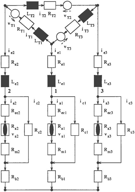
Fig. 2.

Equivalent circuit diagram for the three-phase electrical system in the furnace, reproduced with permission from Valderhaug (1992). Resistive and inductive circuit elements are shown as white and black rectangles, respectively. The white circles denote applied voltages, and the arcs (non-linear resistors) are shown by a black ellipse within a white rectangle.

Open in new tab Download slide

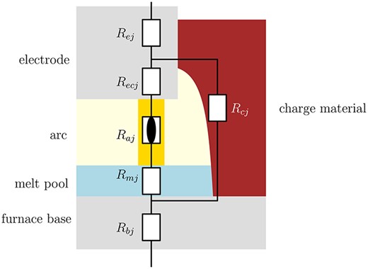
Fig. 3.

Circuit diagram for phase $j$ ⁠, showing the resistance of elements of the electrode, furnace base and furnace hearth.

Open in new tab Download slide

Magnetic fields are generated by the high currents in the furnace, and the changing magnetic fields from the alternating currents have an inductive effect. Following Valderhaug (1992), we assume for simplicity that we may lump the inductances due to both the electrode’s own current (the ‘self-inductance’) and the other currents in the furnace into the single parameter, $L_{j}$ ⁠, for each phase. Similarly, we assume that each transformer has self-inductance $L_{T j}$ ⁠.

The voltage,

v_{T j}

⁠, supplied to each of the transformers

j = 1, 2, 3

is assumed to be a prescribed function of time

t

⁠. As in Valderhaug (1992), we take this to be a standard three-phase system, with

\begin{aligned} v_{T j} (t) = V_{T} \sin (2 π (f t - \frac{j - 1}{3})), \end{aligned}

(2.1)

where

V_{T}

is a prescribed, constant amplitude, and

f

is the frequency of the alternating current. Following Valderhaug (1992), we assume for simplicity that the resistance,

R_{T}

⁠, and self-inductance,

L_{T}

⁠, of each of the three transformers are equal.

The current through phase

j

⁠, equal to the current in electrode

j

⁠, is

i_{e j}

⁠, and the voltage applied across phase

j

is given by

\begin{aligned} v_{j} = R_{j} i_{e j} + L_{j} \frac{d i_{e j}}{d t}, \end{aligned}

(2.2)

where

L_{j}

is the total self-inductance of phase

j

⁠, which we assume is a prescribed constant, and

R_{j}

is the total resistance of phase

j

⁠, given by

\begin{aligned} R_{j} = R_{e j} + R_{b j} + \frac{1}{\frac{1}{R_{c j}} + \frac{1}{R_{e c j} + R_{a j} + R_{m j}}} . \end{aligned}

(2.3)

These resistances are as marked in Fig. 2 and are also shown in Fig. 3.

Using Kirchhoff’s laws for the voltages and currents in the circuit, we may relate the phase voltages

v_{j}

to the voltages across the transformer circuit, and also relate the currents

i_{j}

through each phase to the transformer currents

i_{T j}

⁠. Combining and manipulating these equations to eliminate all

i_{T j}

and

v_{j}

⁠, we may derive the following differential equations for the phase currents:

\begin{aligned} \frac{d i_{e 1}}{d t} = \frac{1}{l_{*}^{2}} ( & (l_{2} + l_{3}) v_{T 1} + l_{2} v_{T 2} + (l_{3} r_{2} - l_{2} r_{3}) i_{e 2} - [(l_{2} + l_{3}) r_{1} + l_{2} r_{3}] i_{e 1}), \end{aligned}

(2.4)

\begin{aligned} \frac{d i_{e 2}}{d t} = \frac{1}{l_{*}^{2}} ( & - l_{3} v_{T 1} + l_{1} v_{T 2} + (l_{3} r_{1} - l_{1} r_{3}) i_{e 1} - [(l_{1} + l_{3}) r_{2} + l_{1} r_{3}] i_{e 2}), \end{aligned}

(2.5)

in terms of the prescribed transformer voltages. The current in the third electrode is simply given by

i_{e 3} = - i_{e 1} - i_{e 2}

⁠. Here, we have defined

\begin{aligned} l_{j} = L_{j} + \frac{L_{T}}{3}, l_{*}^{2} = l_{1} l_{2} + l_{2} l_{3} + l_{1} l_{3}, r_{j} = R_{j} + \frac{R_{T}}{3}, \end{aligned}

(2.6)

for ease of notation.

The two equations (2.4)–(2.5), along with the form (2.3) of the total resistance $R_{j}$ of phase $j$ ⁠, provide a system for the electric currents in each phase. Following Valderhaug (1992), we assume that all the components have constant, prescribed resistances, except for the electric arc. To close the electrical circuit system, we require an equation for each of the arc resistances $R_{a j}$ ⁠. We discuss several models for these arc resistances in the following subsection.

2.2 Modelling the arc resistance

The ionization of the gas in an electric arc, and therefore the electrical resistance of the arc, depend strongly on temperature. Heat is generated in the arc by Ohmic heating due to the electric current, and may be lost to the surroundings by a variety of heat loss mechanisms, including conduction, convection and radiation. Several empirical models for arc resistance are used in the EC models in the SAF literature. In this section, we show how the arc model used in Luckins et al. (2021) may be combined into the EC model presented above. We then compare this arc model with two commonly used empirical arc models, discussing the different structures and parameters in these models.

2.2.1 Arc heat loss due to optically thin radiation

In Luckins et al. (2021), an arc model was presented, based on conservation of energy in the arc region, in which the dominant heat loss from the arc is due to (optically thin) radiation. The arc was modelled as a cylinder of fixed position and size, with radius

r_{a}

and height

h_{a}

⁠, and with spatially uniform temperature

T_{a}

being the solution of the equation of conservation of energy, given by

\begin{aligned} ρ c_{p} \frac{d T_{a}}{d t} = σ_{a} (T_{a}) E^{2} - 4 a σ_{B} T_{a}^{4} . \end{aligned}

(2.7)

Here,

σ_{B} = 5.67 \times 10^{- 8}

^{- 2}

^{- 4}

is the Stefan–Boltzmann constant, while

ρ

[kgm

^{- 3}

] is the density,

c_{p}

[Jkg

^{- 1}

^{- 1}

] is the specific heat capacity and

a

^{- 1}

] is the radiative emission coefficient, these material parameters being assumed to be constant. Reference parameter values for SAF arcs, based on the data given in Luckins et al. (2021), are

\begin{array}{r} ρ = 2 \times 10^{- 2} kg m^{- 3}, c_{p} = 10^{3} J {kg}^{- 1} K^{- 1}, a = 0.1 m^{- 1}, r_{a} = 0.1 m, h_{a} = 0.15 m . \end{array}

(2.8)

The electrical conductivity,

σ_{a} (T_{a})

[

Ω^{- 1}

^{- 1}

] of the arc is an increasing function of temperature. In Luckins et al. (2021), the form

\begin{aligned} σ_{a} (T_{a}) = S_{1} \exp (- \frac{S_{2}}{T_{a}}), \end{aligned}

(2.9)

was used, for constant coefficients

S_{1} = 2.5 \times 10^{4} Ω^{- 1}

^{- 1}

and

S_{2} = 1.8 \times 10^{4}

One benefit of this arc model is that we may easily understand how the energy lost from the arc is transferred to the surrounding material. In Luckins et al. (2021), since the heat radiation was assumed to be optically thin, all the heat radiated by the arc was incident on the surrounding material on the edge of the crater, heating up the charge material. This provided coupling between the fast-timescale equation (2.7) for the arc, and the much slower heat transfer, chemical reactions and material flow in the surrounding charge material. The averaged quantities

\begin{aligned} ⟨ E^{2} ⟩ and ⟨ T_{a}^{4} ⟩ \end{aligned}

(2.10)

were computed from the solution of the fast-timescale model, where the average is defined by

\begin{aligned} ⟨ \cdot ⟩ = f \int_{t = 0}^{1 / f} \cdot d t, \end{aligned}

(2.11)

where

f

is the frequency of the alternating current, and were used in the slow-timescale model.

In Luckins et al. (2021), the electric field,

E

⁠, was a variable to be determined. To fix

E

we imposed a sinusoidal electrode current, with prescribed amplitude. Rather than simply prescribing a sinusoidal electrode current, we may combine our arc model (2.7) into the EC model developed above, as follows. We assume that each of the three arcs have temperature

T_{a j}

satisfying (2.7). To combine our arc model (2.7) with the electric circuit system, we transform (2.7) from an equation for the evolution of the arc temperature

T_{a j}

⁠, to an equation for the evolution of the arc resistance

R_{a j}

⁠, which is defined by

\begin{aligned} R_{a j} = \frac{h_{a}}{π r_{a}^{2} σ_{a} (T_{a j})} = \frac{h_{a}}{S_{1} π r_{a}^{2}} \exp (\frac{S_{2}}{T_{a j}}) . \end{aligned}

(2.12)

We also use the voltage

v_{a j}

across arc

j

⁠, and so make the change of variables

v_{a j} = h_{a} E

⁠. The equation (2.7) then becomes

\begin{aligned} \frac{d R_{a j}}{d t} = \frac{1}{β_{r}} \frac{R_{a j}}{(\log (b R_{a j}))^{2}} (1 - \frac{v_{a j}^{2} \log (b R_{a j})^{4}}{P_{r} R_{a j}}), \end{aligned}

(2.13)

where the parameters

b

[

Ω^{- 1}

β_{r}

[s] and

P_{r}

[Wm

^{- 3}

] are given by

\begin{array}{r} b = \frac{S_{1} π r_{a}^{2}}{h_{a}}, β_{r} = \frac{ρ c_{p}}{4 a σ_{B} S_{2}^{3}}, P_{r} = 4 a σ_{B} S_{2}^{4} π r_{a}^{2} h_{a} . \end{array}

(2.14)

From the electric circuit, we may express the arc voltage

v_{a j}

in terms of

R_{a j}

⁠,

R_{c}

and

i_{e j}

⁠, namely

\begin{aligned} v_{a j} = R_{a j} i_{a j} = R_{a j} \frac{R_{c j}}{R_{e c j} + R_{a j} + R_{m j} + R_{c j}} i_{e j} . \end{aligned}

(2.15)

The equation (2.13) for each phase

j = 1, 2, 3

along with (2.15) closes the electric circuit system presented in the previous section. In our notation, the averaged quantities (2.10) are given by

\begin{array}{r} ⟨ T_{a j}^{4} ⟩ = ⟨ S_{2}^{4} / \log (b R_{a j})^{4} ⟩ and ⟨ (v_{h j})^{2} ⟩, \end{array}

(2.16)

where

v_{h j}

⁠, the voltage across the entire hearth region of phase

j

⁠, is given by

\begin{aligned} v_{h j} = \frac{R_{e c} + R_{m} + R_{a j}}{R_{a j}} v_{a j} . \end{aligned}

(2.17)

This is different from Luckins et al. (2021) only because there the pool and electrode resistances were neglected, and so it was effectively assumed that

R_{m} = R_{e c} = 0

⁠. In order to include our simulations into the homogenized model of Luckins et al. (2021), we require the averaged values (2.16) as functions of the charge resistance

R_{c j}

⁠.

2.2.2 Commonly used models for the arc resistance

Arc models that are commonly used within EC models for SAFs include those due to Cassie (1939) and, less often, Mayr (1943b). Although it is not how they were originally formulated, both of these models may be understood in terms of the total conservation of energy in the arc, namely

\begin{aligned} \frac{d Q_{j}}{d t} = P_{j} - P_{j}^{loss} = \frac{v_{a j}^{2}}{R_{a j}} - P_{j}^{loss}, \end{aligned}

(2.18)

where

Q_{j}

is the heat content in arc

j

⁠, heat is lost through the

P_{j}^{loss}

term and the power generated in the arc is given by the Ohmic heating term

\begin{aligned} P_{j} = \frac{v_{a j}^{2}}{R_{a j}} . \end{aligned}

(2.19)

The different arc models in the literature take different forms for

Q_{j}

and

P_{j}^{loss}

⁠. For instance, for our radiation-based model (2.13), we used the forms

\begin{array}{r} P_{j}^{loss} = 4 a σ_{B} π r_{a}^{2} h_{a} T_{a j}^{4} = \frac{P_{r}}{{(\log (b R_{a j}))}^{4}} and Q_{j} = π r_{a}^{2} h_{a} ρ c_{p} T_{a j} = \frac{β_{r} P_{r}}{\log (b R_{a j})} . \end{array}

(2.20)

We obtain the Cassie model if we take (Gustavsson, 2004; Parizad et al., 2009; Valderhaug, 1992)

\begin{array}{r} P_{j}^{loss} = \frac{U^{2}}{R_{a j}} and Q_{j} = \frac{β_{c}}{U^{2} R_{a j}}, \end{array}

(2.21)

for constants

β_{c}

and

U^{2}

⁠. This model is expected to give a good fit when heat loss from the arc is ‘mainly convective’ (Gustavsson, 2004; Parizad et al., 2009), and is generally held to be a reasonable model for high-current arcs (Bowman & Krüger, 2009; Parizad et al., 2009; Valderhaug, 1992). With these functional forms, the conservation of energy equation (2.18) may be written as

\begin{aligned} \frac{d R_{a j}}{d t} = \frac{R_{a j}}{β_{c}} (1 - {(\frac{v_{a j}}{U})}^{2}) . \end{aligned}

(2.22)

The Mayr model, by contrast, may be obtained with the parameterisation

\begin{array}{r} P_{j}^{loss} = P_{m} and Q_{j} = - \frac{β_{m}}{P_{0}} \log (R_{a j}) . \end{array}

(2.23)

Here, the heat loss

P_{m}

is constant, which is intended to be a good model for conductive heat loss (Gustavsson, 2004; Parizad et al., 2009). The heat content

Q_{j}

is logarithmic in

R_{a j}

⁠, which follows from an assumption that

Q_{j}

is proportional to

T

and that the arc conductivity is proportional to

\exp (T / constant)

⁠. Using (2.23) in the conservation of energy equation, (2.18), gives

\begin{aligned} \frac{d R_{a j}}{d t} = \frac{R_{a j}}{β_{m}} (1 - \frac{v_{a j}^{2}}{P_{m} R_{a j}}) . \end{aligned}

(2.24)

This Mayr model, (2.24), is generally used for low-current arcs (Gustavsson, 2004; Parizad et al., 2009), and so is less often used than the Cassie model in SAF applications.

2.2.3 Discussion and comparison

Along with any of the Cassie (2.22), Mayr (2.24) or radiation (2.13) models, the system of ODEs (2.4)–(2.5) comprise a closed, fully coupled system for the five unknowns $i_{e 1}$ ⁠, $i_{e 2}$ ⁠, $R_{a 1}$ ⁠, $R_{a 2}$ and $R_{a 3}$ ⁠.

Both the Cassie and Mayr models require only two parameters, compared with the three parameters required for the radiation model (2.13). However, the Cassie and Mayr models have the disadvantage that, since they are empirical, the parameters in the model are not directly interpretable in terms of the physical parameters of the system. In addition, the radiation model (2.13) may be used in conjunction with a slow-time model of the charge evolution (Luckins et al., 2021), but it is not clear how the power lost from a Cassie or Mayr arc would correspond to the heating of the surroundings. Furthermore, the Cassie and Mayr were designed to capture the extinction behaviour of circuit-breakers arcs (Gustavsson, 2004), not the SAF arcs which reform every half-period of the AC cycle.

All of these arc models have the arc resistance $R_{a j}$ decreasing with the increase of Ohmic heating, via the $- v_{a j}^{2} F (R_{a j})$ term (for different functions $F$ of $R_{a j}$ in each of (2.13), (2.22) and (2.24)). The functional form $F$ is different for each of the models due to the different choices for the dependence of the heat content, $Q_{j}$ ⁠, of the arc on $R_{a j}$ ⁠.

Since arc resistance decreases with increasing arc temperatures, the heat loss term in (2.18) becomes a source term in each of the equations (2.13), (2.22) and (2.24) for $R_{a j}$ ⁠, while the Ohmic heating becomes a loss term for $R_{a j}$ ⁠. Since $v_{a j}$ ⁠, given by (2.15), depends on both $R_{a j}$ and $i_{e j}$ ⁠, this Ohmic heating term is non-linear for all three of the arc models. The dependences of these terms on $R_{a j}$ are summarized in Table 1.

Table 1

Open in new tab

The source and sink terms in each of the arc models (2.13), (2.22) and (2.24), as functions of the arc resistance $R_{a}$ ⁠.

Model	Radiation	Cassie	Mayr
Source	$\frac{R_{a}}{β_{r} \log (b R_{a})^{2}}$	$\frac{R_{a}}{β_{c}}$	$\frac{R_{a}}{β_{m}}$
Sink	$\frac{i_{e}^{2} R_{c}^{2}}{β_{r} P_{r}} \frac{R_{a}^{2} \log (b R_{a})^{2}}{(R_{a} + R_{c} + R_{m} + R_{e c})^{2}}$	$\frac{i_{e}^{2} R_{c}^{2}}{β_{c} U^{2}} \frac{R_{a}^{3}}{(R_{a} + R_{c} + R_{m} + R_{e c})^{2}}$	$\frac{i_{e}^{2} R_{c}^{2}}{β_{m} P_{m}} \frac{R_{a}^{2}}{(R_{a} + R_{c} + R_{m} + R_{e c})^{2}}$

Table 1

Open in new tab

The source and sink terms in each of the arc models (2.13), (2.22) and (2.24), as functions of the arc resistance $R_{a}$ ⁠.

Model	Radiation	Cassie	Mayr
Source	$\frac{R_{a}}{β_{r} \log (b R_{a})^{2}}$	$\frac{R_{a}}{β_{c}}$	$\frac{R_{a}}{β_{m}}$
Sink	$\frac{i_{e}^{2} R_{c}^{2}}{β_{r} P_{r}} \frac{R_{a}^{2} \log (b R_{a})^{2}}{(R_{a} + R_{c} + R_{m} + R_{e c})^{2}}$	$\frac{i_{e}^{2} R_{c}^{2}}{β_{c} U^{2}} \frac{R_{a}^{3}}{(R_{a} + R_{c} + R_{m} + R_{e c})^{2}}$	$\frac{i_{e}^{2} R_{c}^{2}}{β_{m} P_{m}} \frac{R_{a}^{2}}{(R_{a} + R_{c} + R_{m} + R_{e c})^{2}}$

We may compare these models by examining the steady-state solution(s) of each respective model, which may be thought of as solutions relevant to direct current (DC) arcs. For sufficiently small time-constants $β_{r}$ ⁠, $β_{c}$ and $β_{m}$ ⁠, we expect the AC solution to behave similarly to the steady-state solutions at high current values (we will indeed see that this is the case in our numerical solutions in Section 4). The functional forms of the source terms (due to heat losses) and sink term (due to Ohmic heating), summarised in Table 1, are illustrated in Fig. 4a–c, as functions of the arc resistance, $R_{a}$ ⁠, for each of the three models. The values of $R_{c}$ ⁠, $R_{m}$ ⁠, $R_{e c}$ and the model parameters are considered constants, and we also suppose there is a constant applied current $i_{e}$ ⁠. Steady-state solutions are the intersection(s) of the source and sink curves, and the stability is shown by the arrows in Fig. 4a–c. We note that for all the models, there is no steady-state solution if $i_{e}$ is smaller than some critical value $i_{e}^{crit}$ (which is different for each of the three arc models, and may depend on the other parameters $R_{c}$ ⁠, $R_{m}$ and $R_{e c}$ ⁠). For $i_{e} < i_{e}^{crit}$ ⁠, we expect $R_{a j} \to \infty$ for the dynamic solutions. The Cassie model has a single non-trivial steady-state solution for $i_{e} \geq i_{e}^{crit}$ ⁠, whereas both the Mayr and radiation models may have one non-trivial steady state (when the source and sink curves meet tangentially, at $i_{e} = i_{e}^{crit}$ ⁠) or two non-trivial steady states for $i_{e} > i_{e}^{crit}$ ⁠. All three of the models have exactly one stable steady-state solution, labelled $R_{a}^{*}$ in Fig. 4a–c (although we note that for both the Mayr and radiation models, at the critical current $i_{e}^{crit}$ ⁠, the single steady state is only an attracting point for $R_{a} < R_{a}^{*}$ ⁠, not for $R_{a} > R_{a}^{*}$ ⁠, as the two steady states coalesce into one at this point).

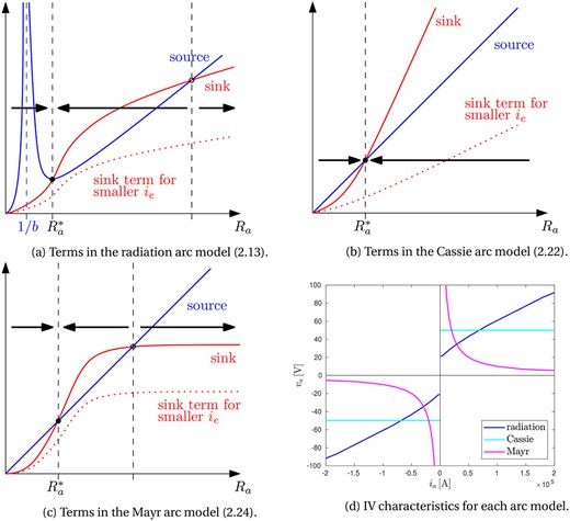
Fig. 4.

Comparison of the arc models. In (a)–(c), for the radiation, Cassie and Mayr models, we give an illustration of the source and sink terms in the arc resistance equation, as in Table 1 and the steady-state solution(s). The black arrows indicate the direction of evolution of dynamic solutions. In (d) we show typical steady-state current-voltage relationships (IV characteristics) for each arc model.

Open in new tab Download slide

We may investigate the arc current–voltage relationship (or ‘IV characteristic’) of the steady-state solutions. At a (non-zero) steady-state solution of the radiation arc model we see from the equation (2.13), and the relationship

i_{a j} = v_{a j} / R_{a j}

that we must have

\begin{aligned} v_{a j} = \pm \sqrt{\frac{P_{r} R_{a j}}{\log (b R_{a j})^{4}}}, i_{a j} = \frac{v_{a j}}{R_{a j}} = \pm \frac{\sqrt{P_{r}}}{\sqrt{R_{a j}} \log (b R_{a j})^{2}} . \end{aligned}

(2.25)

This gives the IV characteristic of the radiation arc model (parameterised by $R_{a j}$ ⁠), which we plot in Fig. 4d. For the Cassie model, we see from the equation (2.22) that steady states require $v_{a j} = \pm U$ to be constant, whereas for the Mayr model (2.24) we must have $v_{a j} = \pm \sqrt{P_{m} R_{a j}}$ ⁠, and so $i_{a j} = v_{a j} / R_{a j} = \pm P_{m} / v_{a j}$ ⁠. These steady-state IV characteristics are plotted for each of the three models in Fig. 4d. We note that since the arc resistance equations depend on $v_{a j}^{2}$ ⁠, both the positive and negative solutions correspond to the same steady state in terms of $R_{a}$ ⁠: the arc resistance does not depend on the direction of the current flow through the arc. All the non-trivial steady-state solutions (stable and unstable) lie on the IV characteristic for that arc model. We may think of the IV characteristic as being parameterised by the electrode current $i_{e}$ ⁠. The three arc models have very different IV characteristics, with the arc voltage $v_{a}$ decreasing for the Mayr model, constant for the Cassie model and increasing for the radiation model, with increasing $i_{a}$ ⁠. At high currents, and for sufficiently fast arc variation (corresponding to sufficiently small $β_{r}$ ⁠, $β_{c}$ or $β_{m}$ ⁠) we expect the AC simulations to follow the steady-state IV characteristics closely, and indeed we observe this behaviour in the numerical simulations in Section 4 below. These differences in the steady-state behaviour are important, as they give insight into the high-current behaviour of the dynamic AC solutions. IV characteristics are found by Saevarsdóttir (2002) for AC simulations of both an MHD arc model, and also for a semi-empirical CAM designed for SAF arcs, which is simpler than the full MHD model, but still considerably more complicated than the Cassie, Mayr or radiation models. Both these more sophisticated models in Saevarsdóttir (2002) show IV characteristics that are rising at high currents, not falling or constant as for the Cassie or Mayr models. This provides some validation for the radiation arc model, which is the only one of the three with a rising steady-state IV characteristic.

2.3 Initial conditions

The model (2.4)–(2.5) along with one of the arc models is a system of first-order ODEs for variables

i_{e j}

and

R_{a j}

⁠. Therefore, to solve the system, we require initial conditions for each of the

i_{e j}

and

R_{a j}

⁠. We are interested in the periodic solutions of the system, and so in practice simply prescribe non-trivial initial conditions for the arc resistances, and solve forward in time until the solution is periodic. In the numerical solutions of Section 4 we prescribe the initial conditions

\begin{aligned} i_{e 1} = i_{e 2} = 0 and R_{a 1} = R_{a 2} = R_{a 3} = R_{0} at t = 0, \end{aligned}

(2.26)

for a constant initial resistance

R_{0}

⁠. As in the previous section, there is exactly one non-trivial steady-state solution for each of the arc models (for sufficiently high

i_{e}

⁠), to which the dynamic solution will evolve during the AC period. We therefore expect that periodic solutions will not depend on the choice of initial conditions, and we indeed find this to be the case in the numerical simulations of Section 4.

2.4 Industrial measurements

In an industrial setting, it is not possible to observe all variables in our model directly: only the total current, $i_{e j}$ ⁠, through each phase, and total voltage $v_{j}$ across each phase $j$ can be measured.

The electrode currents

i_{e j}

are computed as the solution of the model, and the phase voltages

v_{j}

may be found from (2.2), which, using the forms of

d i_{e j} / d t

from (2.4)–(2.5), may be expressed as

\begin{aligned} v_{1} & = R_{1} i_{e 1} + \frac{L_{1}}{l_{*}^{2}} ((l_{2} + l_{3}) v_{T 1} + l_{2} v_{T 2} + (l_{3} r_{2} - l_{2} r_{3}) i_{e 2} - [(l_{2} + l_{3}) r_{1} + l_{2} r_{3}] i_{e 1}), \end{aligned}

(2.27a)

\begin{aligned} v_{2} & = R_{2} i_{e 2} + \frac{L_{2}}{l_{*}^{2}} (- l_{3} v_{T 1} + l_{1} v_{T 2} + (l_{3} r_{1} - l_{1} r_{3}) i_{e 1} - [(l_{1} + l_{3}) r_{2} + l_{1} r_{3}] i_{e 2}), \end{aligned}

(2.27b)

\begin{aligned} v_{3} & = R_{3} (- i_{e 1} - i_{e 2}) + \frac{L_{3}}{l_{*}^{2}} ((l_{2} r_{1} + (l_{2} + l_{1}) r_{3}) i_{e 1} + (l_{1} r_{2} + (l_{1} + l_{2}) r_{3}) i_{e 2} + l_{2} v_{T 1} + (l_{1} + l_{2}) v_{T 2}) . \end{aligned}

(2.27c)

3. Nondimensionalization

We now nondimensionalize the EC model and each of the three arc models presented in Section 2, using industrially relevant parameter values. We discuss the dimensionless parameters at the end of this section, before solving the dimensionless model numerically in Section 4.

We nondimensionalize the system (2.4)–(2.5), (2.3), (2.15) and the arc resistance equation (either (2.13), (2.22) or (2.24)) using the rescalings

\begin{aligned} t = \frac{1}{f} \hat{t}, & v_{a j} = V_{T} {\hat{v}}_{a j}, & i_{e j} = [i] {\hat{i}}_{j}, & R_{c j} = \frac{V_{T}}{[i]} {\hat{R}}_{c j}, & R_{a j} = \frac{V_{T}}{[i]} {\hat{R}}_{a j}, & R_{j} = \frac{V_{T}}{[i]} {\hat{R}}_{j}, & r_{j} = \frac{V_{T}}{[i]} {\hat{r}}_{j}, \end{aligned}

(3.1)

where the hat notation denotes dimensionless variables. We have chosen the timescale of the alternating current, prescribed the current scaling to be

[i]

⁠, and chosen the scalings of the resistances so that the voltage drop due to resistance balances the forcing due to the transformer voltages in (2.4)–(2.5). Using these rescalings, the dimensionless system (dropping the hat notation) is

\begin{aligned} ζ_{I} \frac{d i_{1}}{d t} & = (1 + λ_{2}) \sin (2 π t) + λ_{2} \sin (2 π (t - \frac{1}{3})) + (r_{2} - λ_{2} r_{3}) i_{2} - ((1 + λ_{2}) r_{1} + λ_{2} r_{3}) i_{1}, \end{aligned}

(3.2a)

\begin{aligned} ζ_{I} \frac{d i_{2}}{d t} & = - \sin (2 π t) + λ_{1} \sin (2 π (t - \frac{1}{3})) + (r_{1} - λ_{1} r_{3}) i_{1} - ((1 + λ_{1}) r_{2} + λ_{1} r_{3}) i_{2}, \end{aligned}

(3.2b)

where

\begin{array}{r} i_{3} = - i_{1} - i_{2}, and r_{j} = r_{e j} + \frac{1}{\frac{1}{R_{c j}} + \frac{1}{r_{c r j} + R_{a j}}}, v_{a j} = \frac{R_{a j} R_{c j} i_{j}}{R_{a j} + R_{c j} + r_{c r j}}, for j = 1, 2, 3, \end{array}

(3.3)

along with one of the following arc models:

\begin{aligned} Radiation: ζ_{r} \frac{d R_{a j}}{d t} = \frac{R_{a j}}{\log (B R_{a j})^{2}} (1 - \frac{v_{a j}^{2} \log (B R_{a j})^{4}}{p_{r} R_{a j}}), \end{aligned}

(3.4a)

\begin{aligned} Cassie: ζ_{c} \frac{d R_{a j}}{d t} = R_{a j} (1 - \frac{v_{a j}^{2}}{p_{c}}), \end{aligned}

(3.4b)

\begin{aligned} Mayr: ζ_{m} \frac{d R_{a j}}{d t} = R_{a j} (1 - \frac{v_{a j}^{2}}{p_{m} R_{a j}}) . \end{aligned}

(3.4c)

Here, we have introduced the dimensionless parameters for the electrical system,

\begin{aligned} ζ_{I} = \frac{l_{*}^{2} f [i]}{l_{3} V_{T}}, & λ_{1} = \frac{l_{1}}{l_{3}}, λ_{2} = \frac{l_{2}}{l_{3}}, \\ r_{e j} = \frac{[i]}{V_{T}} (R_{e j} + R_{b j} + \frac{R_{T}}{3}), & r_{c r j} = \frac{[i]}{V_{T}} (R_{e c j} + R_{m j}), for j = 1, 2, 3, \end{aligned}

(3.5)

and, depending on the choice of arc model used, the dimensionless parameters, for

j = 1, 2, 3

⁠,

\begin{aligned} Radiation: ζ_{r j} = β_{r j} f, p_{r j} = \frac{P_{r j}}{V_{T} [i]}, B_{j} = \frac{b_{j} V_{T}}{[i]}, \end{aligned}

(3.6)

\begin{aligned} Cassie: ζ_{c j} = β_{c j} f, p_{c j} = \frac{U_{c j}^{2}}{V_{T}^{2}}, \end{aligned}

(3.7)

\begin{aligned} Mayr: ζ_{m j} = β_{m j} f, p_{m j} = \frac{P_{m j}}{V_{T} [i]} . \end{aligned}

(3.8)

For comparison with industrial measurements, we also nondimensionalize (2.27), using the additional scaling

\begin{aligned} v_{j} & = V_{T} {\hat{v}}_{j} . \end{aligned}

(3.9)

Dropping the hat notation, this gives

\begin{aligned} v_{1} = & (r_{1} - μ) i_{1} + \frac{λ_{1} - λ_{T}}{λ_{1} + λ_{2} + λ_{1} λ_{2}} ((λ_{2} + 1) \sin (2 π t) + λ_{2} \sin (2 π (t - \frac{1}{3})) \\ + (r_{2} - λ_{2} r_{3}) i_{2} - ((λ_{2} + 1) r_{1} + λ_{2} r_{3}) i_{1}), \end{aligned}

(3.10a)

\begin{aligned} v_{2} = & (r_{2} - μ) i_{2} + \frac{λ_{2} - λ_{T}}{λ_{1} + λ_{2} + λ_{1} λ_{2}} (- \sin (2 π t) + λ_{1} \sin (2 π (t - \frac{1}{3})) \\ + (r_{1} - λ_{1} r_{3}) i_{1} - ((λ_{1} + 1) r_{2} + λ_{1} r_{3}) i_{2}), \end{aligned}

(3.10b)

\begin{aligned} v_{3} = & (r_{3} - μ) (- i_{1} - i_{2}) + \frac{λ_{2} (1 - λ_{T})}{λ_{1} + λ_{2} + λ_{1} λ_{2}} [(r_{1} + (1 + \frac{λ_{1}}{λ_{2}}) r_{3}) i_{1} + (\frac{λ_{1}}{λ_{2}} r_{2} + (\frac{λ_{1}}{λ_{2}} + 1) r_{3}) i_{2} \\ + \sin (2 π t) + (\frac{λ_{1}}{λ_{2}} + 1) \sin (2 π (t - \frac{1}{3}))], \end{aligned}

(3.10c)

where we have introduced the additional dimensionless parameters

\begin{aligned} μ = \frac{R_{T} [i]}{3 V_{T}} and λ_{T} = \frac{L_{T}}{3 l_{3}} . \end{aligned}

(3.11)

We use

S_{2}

(defined in (2.9)) as the scaling for the arc temperature

T_{a j}

⁠, and

V_{T}

as the scaling for

v_{h j}

⁠. Dropping the hat notation, the dimensionless averaged quantities (2.16) then become

\begin{array}{r} ⟨ 1 / \log (B R_{a j})^{4} ⟩ and ⟨ (v_{j}^{h})^{2} ⟩, \end{array}

(3.12)

where

\begin{aligned} ⟨ \cdot ⟩ := \int_{t = 0}^{1} \cdot d t \end{aligned}

(3.13)

is the dimensionless time-average.

Physically relevant data values are given in Table 2, including the sizes of the radiation parameters given by (2.14) using industrially relevant data values (Luckins et al., 2021). Since the parameters for the Cassie and Mayr models are empirical, and must be chosen to fit data, we do not include these in Table 2. Using the data of Table 2, the corresponding values for the dimensionless parameters are listed in Table 3.

Table 2

Open in new tab

Industrially relevant data values used for the nondimensionalization. The arc parameters $β_{r}$ ⁠, $P_{r}$ and $b$ are computed using data collated in Luckins et al. (2021).

Parameter/Scaling	Value
$f$	$50$ s $^{- 1}$
$V_{T}$	$260 \sqrt{2}$ V
$[i]$	$1.65 \times 10^{5}$ A
$R_{e}$	$1 \times 10^{- 4} Ω$
$R_{b}$	$3 \times 10^{- 4} Ω$
$R_{m}$	$1 \times 10^{- 4} Ω$
$R_{e c}$	$2 \times 10^{- 5} Ω$
$R_{T}$	$1.0 \times 10^{- 7} Ω$
$L$	$2.0 \times 10^{- 6} Ω$ s
$L_{T}$	$6.3 \times 10^{- 7} Ω$ s
$P_{r}$	$1.1 \times 10^{7}$ Wm $^{- 3}$
$β_{r}$	$1.5 \times 10^{- 4}$ s
$b$	$5.2 \times 10^{3} Ω^{- 1}$

Table 2

Open in new tab

Industrially relevant data values used for the nondimensionalization. The arc parameters $β_{r}$ ⁠, $P_{r}$ and $b$ are computed using data collated in Luckins et al. (2021).

Parameter/Scaling	Value
$f$	$50$ s $^{- 1}$
$V_{T}$	$260 \sqrt{2}$ V
$[i]$	$1.65 \times 10^{5}$ A
$R_{e}$	$1 \times 10^{- 4} Ω$
$R_{b}$	$3 \times 10^{- 4} Ω$
$R_{m}$	$1 \times 10^{- 4} Ω$
$R_{e c}$	$2 \times 10^{- 5} Ω$
$R_{T}$	$1.0 \times 10^{- 7} Ω$
$L$	$2.0 \times 10^{- 6} Ω$ s
$L_{T}$	$6.3 \times 10^{- 7} Ω$ s
$P_{r}$	$1.1 \times 10^{7}$ Wm $^{- 3}$
$β_{r}$	$1.5 \times 10^{- 4}$ s
$b$	$5.2 \times 10^{3} Ω^{- 1}$

Table 3

Open in new tab

Dimensionless parameters, computed using the data in Table 2.

Dimensionless parameter	Value
$ζ_{I}$	$1.3 \times 10^{- 1}$
$r_{e}$	$1.8 \times 10^{- 1}$
$r_{c r}$	$5.4 \times 10^{- 2}$
$ζ_{r}$	$7.6 \times 10^{- 3}$
$p_{r}$	$1.8 \times 10^{- 1}$
$B$	$1.2 \times 10$
$μ$	$1.4 \times 10^{- 5}$
$λ_{T}$	$1.1 \times 10^{- 1}$
$λ_{1}, λ_{2}$	$\approx 1$

Table 3

Open in new tab

Dimensionless parameters, computed using the data in Table 2.

Dimensionless parameter	Value
$ζ_{I}$	$1.3 \times 10^{- 1}$
$r_{e}$	$1.8 \times 10^{- 1}$
$r_{c r}$	$5.4 \times 10^{- 2}$
$ζ_{r}$	$7.6 \times 10^{- 3}$
$p_{r}$	$1.8 \times 10^{- 1}$
$B$	$1.2 \times 10$
$μ$	$1.4 \times 10^{- 5}$
$λ_{T}$	$1.1 \times 10^{- 1}$
$λ_{1}, λ_{2}$	$\approx 1$

We notice that, as expected, both $r_{c r}$ and $r_{e}$ are relatively small, so that the resistance of the charge material or of the arc dominates the total resistance through each phase. The value $μ$ is negligibly small, and so we may neglect the effect of the transformer resistances when computing the phase voltages $v_{j}$ in (3.10). The inductance of the transformers is small, but not negligible in comparison with the electrode inductances, since $λ_{T} \approx 0.11$ ⁠. The asymmetry of the system is encoded in the parameters $λ_{1}, λ_{2}$ (which are both 1 if the electrode inductances are equal), the different values of $r_{e j}$ ⁠, $r_{c r j}$ and the arc parameters $B_{j}$ ⁠, $ζ_{r j}$ and $p_{r j}$ (or equivalent arc parameters for the Cassie or Mayr models).

We note that the inductance effects, captured by the parameter $ζ_{I}$ ⁠, are relatively small. Furthermore, the timescale $ζ_{r}$ of the variation in the arc resistance is very small, although, as we found in Luckins et al. (2021), this does not necessarily mean that the arc behaviour is quasi-steady, since both the Ohmic heating and heat loss effects are temperature dependent, and are much slower at lower temperatures. Since both $ζ_{I}$ and especially $ζ_{r}$ are small, we anticipate some stiffness in the ODE system.

4. Numerical solutions

In this section, we present the results of our the numerical simulations of the system (3.2) with each of the arc models (3.4). Numerical solutions are found using Matlab, where we employ the in-built ODE solver ode15s, which is a multistep solver, using numerical differentiation formulas of order 1–5 (Shampine & Reichelt, 1997). In particular, this solver is designed to deal with stiff ODE systems (Shampine & Reichelt, 1997). As discussed in Section 2.3, we initialize at the (appropriately nondimensionalized) initial conditions (2.26), and solve forward in time until the solutions are periodic (usually within one or two periods). We observe that the periodic solution is independent of the choice of initial value $R_{0}$ ⁠, so long as this is sufficiently large that periodic solutions may be found.

We have made several simplifying assumptions in the model presented above, but there are still a large number of dimensionless parameters in the model. For simplicity, in the majority of this section we restrict to a symmetric model, assuming that all the parameters (including the arc parameters) for each of the three phases are equal. Specifically, we set $λ_{1} = λ_{2} = 1,$ and use the notation $R_{c}$ ⁠, $r_{e}$ ⁠, $r_{c r}$ ⁠, $ζ_{r}$ ⁠, $p_{r}$ ⁠, $B$ ⁠, $ζ_{c}$ ⁠, $p_{c}$ ⁠, $ζ_{m}$ and $p_{m}$ for each of $R_{c j}$ ⁠, $r_{e j}$ ⁠, $r_{c r j}$ ⁠, $ζ_{r j}$ ⁠, $p_{r j}$ ⁠, $B_{j}$ ⁠, $ζ_{c j}$ ⁠, $p_{c j}$ ⁠, $ζ_{m j}$ and $p_{m j}$ ⁠, for $j = 1, 2, 3$ ⁠, respectively. In Sections 4.1–4.5, when the system is symmetric, we only present solutions for phase 1; the solutions for the other phases are the same up to phase shift. Solutions including asymmetric parameter values are found in Section 4.6.

4.1 The radiation arc model

Periodic numerical solutions of the system using the radiation arc model (3.4a) are shown in Fig. 5, where we vary the arc-model parameters $p_{r}$ and $ζ_{r}$ ⁠, while holding $B$ ⁠, and the parameters of the external electric circuit, constant. In Fig. 5a, c and e we show the currents through the electrode $i_{1}$ ⁠, arc $i_{a 1} = v_{a 1} / R_{a 1}$ and the charge material $i_{c 1} = v_{h 1} / R_{c}$ for various $p_{r}$ and $ζ_{r}$ ⁠, and in Fig. 5b, d and f we show the associated ‘arc signature’ plots of arc current $i_{a 1}$ against arc voltage $v_{a 1}$ ⁠. Industrially, arc signature is constructed from the furnace measurements, and the shape is used to infer the internal current distribution of the furnace.

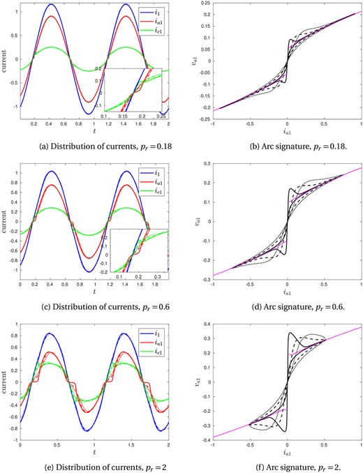
$Numerical solutions using the radiation arc model (3.4a), varying $p_r$ and $\zeta _r$. In (a), (c) and (e), the currents are shown through the electrode ($i_{1}$, blue), arc ($i_{a1}$, red) and charge ($i_{c1}$, green) of phase 1. The insets in (a) and (c) show detail near current zero. In (b), (d) and (f), the arc signature (arc voltage against arc current) is shown. The thin pink curves show the ‘steady state’ or DC solution of the radiation arc model (3.4a). In all plots (a)–(f), the solid lines correspond to $\zeta _r=1\times 10^{-3}$, the dashed lines to $\zeta _r=7.6\times 10^{-3}$ and the dotted lines to $\zeta _r=2\times 10^{-2}$. We take $B=12$ and $R_c=1$, and choose the circuit parameters $\zeta _I=0.13$, $r_{cr}=0.054$, $r_e=0.18$ throughout.$

Fig. 5.

Numerical solutions using the radiation arc model (3.4a), varying $p_{r}$ and $ζ_{r}$ ⁠. In (a), (c) and (e), the currents are shown through the electrode (⁠ $i_{1}$ ⁠, blue), arc (⁠ $i_{a 1}$ ⁠, red) and charge (⁠ $i_{c 1}$ ⁠, green) of phase 1. The insets in (a) and (c) show detail near current zero. In (b), (d) and (f), the arc signature (arc voltage against arc current) is shown. The thin pink curves show the ‘steady state’ or DC solution of the radiation arc model (3.4a). In all plots (a)–(f), the solid lines correspond to $ζ_{r} = 1 \times 10^{- 3}$ ⁠, the dashed lines to $ζ_{r} = 7.6 \times 10^{- 3}$ and the dotted lines to $ζ_{r} = 2 \times 10^{- 2}$ ⁠. We take $B = 12$ and $R_{c} = 1$ ⁠, and choose the circuit parameters $ζ_{I} = 0.13$ ⁠, $r_{c r} = 0.054$ ⁠, $r_{e} = 0.18$ throughout.

Open in new tab Download slide

In general, near to the points where the total current passes through zero, almost all the current passes through the charge. As the arc heats up, it becomes less resistive, and current begins to pass through the arc. The arc signature takes a figure-of-eight shape due to the asymmetry in the increasing- and decreasing-current halves of the AC cycle. As the total current increases from zero, the voltage across the arc increases quickly before it is sufficiently hot to be a good conductor. The arc current then increases, with the arc signature evolving towards the steady-state IV characteristic (discussed in Section 2.2.3), shown by the thin pink lines in Fig. 5. On the decreasing-current half of the cycle, there is a time-delay in the arc cooling, so that it remains warm with relatively low resistance, and hence the arc-signature curve approaches the origin from below the steady-state curve.

Varying $ζ_{r}$ affects the rate at which the arc adapts to the changing voltage across it, so that for small $ζ_{r}$ (solid lines in Fig. 5) the arc adapts very quickly, whereas for larger $ζ_{r}$ (dotted lines) there is a much slower evolution. This is most clearly visible in Fig. 5b, d and f, where increasing $ζ_{r}$ smooths out the shape of the arc signature. However, varying $ζ_{r}$ does not appear to significantly affect the overall current distribution between the arc and the charge, nor the total current $i_{1}$ ⁠.

For small $p_{r}$ ⁠, the arc resistance drops very quickly after the total current passes through zero, so that there is only a small time interval after the total current is zero for which the arc current is low. As $p_{r}$ is increased, so that the Ohmic heat source is smaller, we see that the current is charge-dominated for a longer time after the total current passes through zero, as it takes longer to heat up the arc. Because the arc is cooler for larger $p_{r}$ ⁠, it varies more slowly with the applied voltage, and so we see a bigger effect of varying $ζ_{r}$ ⁠. For larger $p_{r}$ we also observe that a smaller proportion of current passes through the arc, and more through the charge. However, from Fig. 5b, d and f we see that the maximum arc voltage increases with increasing $p_{r}$ ⁠, and the maximum arc current decreases, so that the overall gradient of the arc signature is steeper. We also see from Fig. 5a, c and e that the amplitude of the total current $i_{1}$ decreases as $p_{r}$ increases.

In Fig. 6, we investigate the effect of varying the parameter $B$ ⁠, for fixed $p_{r}$ and $β_{r}$ ⁠. We note that for larger $B$ there is a higher amplitude of the total current $i_{1}$ ⁠, as well as a larger arc current $i_{a 1}$ ⁠. The amplitude of the charge current $i_{c 1}$ decreases as $B$ increases. From the definition (2.14) of the arc parameters, we see that $B$ is proportional to the conductivity magnitude $S_{1}$ of the gas forming the arc. It is therefore natural that larger values of $B$ ⁠, corresponding to more conductive gases, result in larger currents through the arc. We note that for sufficiently small $B$ (below around 8 for the parameters used in Fig. 6), or for sufficiently large $p_{r}$ (larger than the values chosen in Fig. 5), the periodic solution of our model has no current through the arc, so that $i_{a 1} = 0$ for all time $t$ ⁠, and $i_{c 1} = i_{1}$ ⁠. Since $B$ is proportional to $S_{1}$ ⁠, a poorly conductive gas will correspond to small $B$ ⁠, and so no arc forms. We also note that $p_{r}$ is linearly proportional to $h_{a}$ ⁠, the height or length of the electric arc, and $B$ is inversely proportional to $h_{a}$ ⁠. For a fixed gas composition, increasing $h_{a}$ therefore has the effect of both decreasing $B$ and increasing $p_{r}$ ⁠. We therefore expect no solution to exist for sufficiently big arc lengths $h_{a}$ ⁠, as is indeed seen in practice.

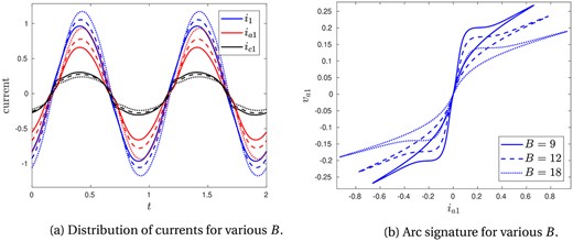
$Numerical solutions using the radiation arc model (3.4a), varying parameter $B$. In (a) the currents are shown through the electrode ($i_{1}$, blue), arc ($i_{a1}$, red) and charge ($i_{c1}$, black) of phase 1, with solid lines ($B=9$), dashed lines ($B=12$) and dotted lines ($B=18$) as in (b). In (b) the arc signature is shown for each value of $B$ in (a). In both plots, we take $p_r=1$, $\zeta _r=7.6\times 10^{-3}$, $R_c=1$, and choose the circuit parameters $\zeta _I=0.13$, $r_{cr}=0.054$, $r_e=0.18$.$

Fig. 6.

Numerical solutions using the radiation arc model (3.4a), varying parameter $B$ ⁠. In (a) the currents are shown through the electrode (⁠ $i_{1}$ ⁠, blue), arc (⁠ $i_{a 1}$ ⁠, red) and charge (⁠ $i_{c 1}$ ⁠, black) of phase 1, with solid lines (⁠ $B = 9$ ⁠), dashed lines (⁠ $B = 12$ ⁠) and dotted lines (⁠ $B = 18$ ⁠) as in (b). In (b) the arc signature is shown for each value of $B$ in (a). In both plots, we take $p_{r} = 1$ ⁠, $ζ_{r} = 7.6 \times 10^{- 3}$ ⁠, $R_{c} = 1$ ⁠, and choose the circuit parameters $ζ_{I} = 0.13$ ⁠, $r_{c r} = 0.054$ ⁠, $r_{e} = 0.18$ ⁠.

Open in new tab Download slide

4.2 Cassie and Mayr arc models

Using the same electric circuit parameters as in the previous section, we now investigate solutions of (3.2) using the Cassie (3.4b) and Mayr (3.4c) arc models instead of the radiation arc model. In Fig. 7, we show solutions of (3.2) using the Cassie model (3.4b) and varying the Cassie parameters.

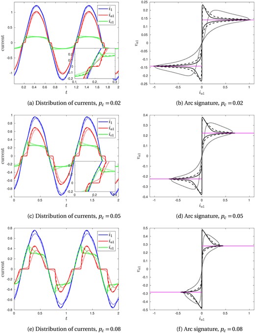
$Numerical solutions using the Cassie arc model (3.4b), varying $p_c$ and $\zeta _c$. In (a), (c) and (e), the currents are shown through the electrode ($i_{1}$, blue), arc ($i_{a1}$, red) and charge ($i_{c1}$, green) of phase 1. The insets in (a) and (c) show detail near to where the current is equal to zero. In (b), (d) and (f) the arc signature (arc voltage against arc current) is shown, along with the steady-state (DC) solution $v_{a1}=\pm \sqrt{p_c}$ in pink. In all plots (a)–(f), the solid lines correspond to $\zeta _c=5\times 10^{-3}$, the dashed lines to $\zeta _c=1\times 10^{-2}$ and the dotted lines to $\zeta _c=5\times 10^{-2}$. We take $R_c=1$, and the circuit parameters $\zeta _I=0.13$, $r_{cr}=0.054$, $r_e=0.18$ throughout.$

Fig. 7.

Numerical solutions using the Cassie arc model (3.4b), varying $p_{c}$ and $ζ_{c}$ ⁠. In (a), (c) and (e), the currents are shown through the electrode (⁠ $i_{1}$ ⁠, blue), arc (⁠ $i_{a 1}$ ⁠, red) and charge (⁠ $i_{c 1}$ ⁠, green) of phase 1. The insets in (a) and (c) show detail near to where the current is equal to zero. In (b), (d) and (f) the arc signature (arc voltage against arc current) is shown, along with the steady-state (DC) solution $v_{a 1} = \pm \sqrt{p_{c}}$ in pink. In all plots (a)–(f), the solid lines correspond to $ζ_{c} = 5 \times 10^{- 3}$ ⁠, the dashed lines to $ζ_{c} = 1 \times 10^{- 2}$ and the dotted lines to $ζ_{c} = 5 \times 10^{- 2}$ ⁠. We take $R_{c} = 1$ ⁠, and the circuit parameters $ζ_{I} = 0.13$ ⁠, $r_{c r} = 0.054$ ⁠, $r_{e} = 0.18$ throughout.

Open in new tab Download slide

We observe qualitatively similar behaviour of solutions using the Cassie model and those using the radiation model in Fig. 5. In the same way as when increasing $p_{r}$ in the radiation model, we see that increasing $p_{c}$ in the Cassie model has the effect of decreasing both the total current $i_{1}$ and the proportion of current through the arc. Increasing $ζ_{c}$ also has the effect of increasing the delay time of the arc, and therefore smooths out the arc signature plots. The main qualitative difference between solutions using the Cassie model in Fig. 7 and the radiation model in Fig. 5 is the slope of the arc signature at high current/voltage, which now follows the constant $v_{a}$ steady-state IV characteristic, shown in pink, as discussed in Section 2.2.3.

Solutions of (3.2) using the Mayr model (3.4c) are shown in Fig. 8. We find limited qualitative variation in the solutions with the parameters $ζ_{m}$ and $p_{m}$ ⁠, for the values of these parameters for which periodic solutions appear to exist. In particular, the arc signatures do not seem to follow the steady-state (DC) curves closely. This is likely to be because we require relatively large values of $ζ_{m}$ in order to observe numerically periodic solutions.

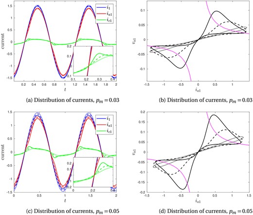
$Numerical solutions using the Mayr arc model (3.4c), varying $p_m$ and $\zeta _m$. In (a) and (c), the currents are shown through the electrode ($i_{1}$, blue), arc ($i_{a1}$, red) and charge ($i_{c1}$, green) of phase 1. The insets in (a) and (c) show detail near to where the current is zero. In (b) and (d), the arc signature (arc voltage against arc current) is shown, along with the steady-state (DC) solution $v_{a1}=p_m/i_{a1}$ in pink. In all plots (a)–(d), the solid lines correspond to $\zeta _m=0.05$, the dashed lines to $\zeta _m=0.1$ and the dotted lines to $\zeta _m=0.5$. For all plots, we take $R_c=1$, and choose the circuit parameters $\zeta _I=0.13$, $r_{cr}=0.054$, $r_e=0.18$.$

Fig. 8.

Numerical solutions using the Mayr arc model (3.4c), varying $p_{m}$ and $ζ_{m}$ ⁠. In (a) and (c), the currents are shown through the electrode (⁠ $i_{1}$ ⁠, blue), arc (⁠ $i_{a 1}$ ⁠, red) and charge (⁠ $i_{c 1}$ ⁠, green) of phase 1. The insets in (a) and (c) show detail near to where the current is zero. In (b) and (d), the arc signature (arc voltage against arc current) is shown, along with the steady-state (DC) solution $v_{a 1} = p_{m} / i_{a 1}$ in pink. In all plots (a)–(d), the solid lines correspond to $ζ_{m} = 0.05$ ⁠, the dashed lines to $ζ_{m} = 0.1$ and the dotted lines to $ζ_{m} = 0.5$ ⁠. For all plots, we take $R_{c} = 1$ ⁠, and choose the circuit parameters $ζ_{I} = 0.13$ ⁠, $r_{c r} = 0.054$ ⁠, $r_{e} = 0.18$ ⁠.

Open in new tab Download slide

4.3 The circuit parameters

In this section, we return to using the radiation arc model (3.4a), but hold the parameters $p_{r}$ ⁠, $B$ and $ζ_{r}$ fixed. Instead, we now investigate the effect of varying the circuit parameters $ζ_{I}$ and $r_{e}$ ⁠. Solutions of (3.2) with (3.4a) are shown in Fig. 9. We observe in Fig. 9a that increasing the inductance $ζ_{I}$ has the effect of decreasing all of the arc, charge and total currents, since a greater proportion of the applied transformer voltage is lost to inductive effects. This effect is also visible in the arc signatures shown in Fig. 9c. For larger $ζ_{I}$ we also see an increased phase shift in Fig. 9a. Increasing the resistance $r_{e}$ in the electrode or base of the furnace is also seen to decrease all the currents, as shown in Fig. 9b and d. However, there is now a (relative) phase shift to the left with increasing $r_{e}$ ⁠. This is because the overall resistance $R_{1}$ is greater, and so the induction effect must account for a smaller proportion of the total applied transformer voltage. We note that we have not explored the dependence of the system on $r_{c r}$ since, as discussed in Section 3, this parameter is expected to be small, and so will have a small effect on the overall solution of the system.

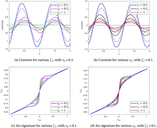
$Numerical solutions using the radiation arc model (3.4a), varying the circuit parameters $\zeta _I$ and $r_e$. In (a) and (b) the currents are shown through the electrode ($i_{1}$, solid), arc ($i_{a1}$, dashed) and charge ($i_{c1}$, dotted) of phase 1. The corresponding arc signatures are shown in (c) and (d). In (a) and (c), $\zeta _I$ is varied, with $r_e=0.1$ constant. In (b) and (d), $r_e$ is varied, with $\zeta _I=0.1$ constant. In all, the arc parameters are $p_r=0.5$, $\zeta _r=7.6\times 10^{-3}$, $B=12$, and we use $R_c=1$ and $r_{cr}=0.054$.$

Fig. 9.

Numerical solutions using the radiation arc model (3.4a), varying the circuit parameters $ζ_{I}$ and $r_{e}$ ⁠. In (a) and (b) the currents are shown through the electrode (⁠ $i_{1}$ ⁠, solid), arc (⁠ $i_{a 1}$ ⁠, dashed) and charge (⁠ $i_{c 1}$ ⁠, dotted) of phase 1. The corresponding arc signatures are shown in (c) and (d). In (a) and (c), $ζ_{I}$ is varied, with $r_{e} = 0.1$ constant. In (b) and (d), $r_{e}$ is varied, with $ζ_{I} = 0.1$ constant. In all, the arc parameters are $p_{r} = 0.5$ ⁠, $ζ_{r} = 7.6 \times 10^{- 3}$ ⁠, $B = 12$ ⁠, and we use $R_{c} = 1$ and $r_{c r} = 0.054$ ⁠.

Open in new tab Download slide

4.4 Comparison with furnace data

Having explored the dependence of our solutions on the model parameters, we now compare the solution of our model with measurements from an operational silicon furnace, with data provided by Elkem ASA. We use parameter values for both the circuit and arc model based on the physical values in Table 3.

We note that there are two additional dimensionless parameters, $μ$ and $λ_{T}$ ⁠, which appear in the form of the phase voltages $v_{j}$ (3.10), which were not needed in the solution of the ODE system (3.2) with the arc model. The parameters $μ$ and $λ_{T}$ describe, respectively, the proportion of the total resistance, and proportion of the total inductance that is due to the transformer circuit. From the industrially relevant data given in Section 3, we see that $μ \approx 10^{- 5}$ ⁠, and so the transformer circuit is responsible for a negligible contribution to the overall resistance. We therefore take the limit $μ = 0$ for our simulations in this section.

The effect of the transformer inductance, while smaller than the electrode inductance, is not negligible. In Fig. 10 we plot the same solution of the (3.2) and (3.4a), but for multiple values of $λ_{T}$ ⁠, and compare these solutions with the furnace data. Specifically, in order to compare with the furnace data we show the Lissajous plot of total current $i_{1}$ against the voltage $v_{1}$ across phase 1 in Fig. 10c, not the arc signature plots of $i_{a 1}$ against $v_{a 1}$ used in Figs 5–9. In the (unphysical) case of $λ_{T} = 1$ (where all of the inductive effect is in the transformer and none is in the electrode), we see from (3.10) that the voltage is purely resistive, $v_{j} = i_{j} R_{j}$ ⁠. The voltage $v_{1}$ is therefore in phase with the electrode current $i_{1}$ ⁠, as seen by the fact that the Lissajous curve in Fig. 10c passes through the origin. For smaller $λ_{T}$ ⁠, there is non-zero induction within the electrode, introducing a phase shift in $v_{1}$ relative to $i_{1}$ ⁠. This phase shift is most easily seen as the width of the Lissajous plot, shown in Fig. 10c. The overall gradient of the Lissajous plot is loosely interpretable as the overall resistance.

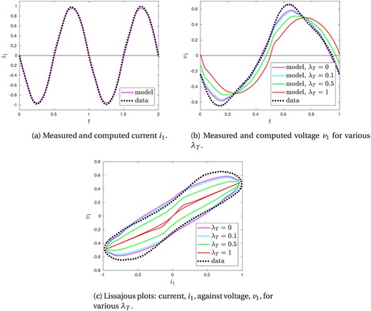
$Comparison of furnace measurements with numerical simulations using the radiation arc model, with arc parameters $p_r=0.2$, $\zeta _r=8\times 10^{-3}$, $B=10$, circuit parameters $\zeta _I=0.13$, $r_e=0.22$ and $r_{cr}=0.054$, and where we have chosen $R_c=2.5$ for reasonable agreement with the data.$

Fig. 10.

Comparison of furnace measurements with numerical simulations using the radiation arc model, with arc parameters $p_{r} = 0.2$ ⁠, $ζ_{r} = 8 \times 10^{- 3}$ ⁠, $B = 10$ ⁠, circuit parameters $ζ_{I} = 0.13$ ⁠, $r_{e} = 0.22$ and $r_{c r} = 0.054$ ⁠, and where we have chosen $R_{c} = 2.5$ for reasonable agreement with the data.

Open in new tab Download slide

The parameters of the arc model (3.4a) used in Fig. 10 are those listed in Table 3, based on physical values in Table 2. There is a reasonable qualitative agreement in the overall shape of the solutions, especially for $λ_{T} = 0.1$ ⁠. The predominant difference between the simulation and data is the shape of the voltage curve near its peak, where our model solution is significantly below the measured data. This indicates that our arc model has a faster reduction in the arc resistance at high voltage than is the case in reality. From our arc-parameter investigation in Section 4.1, we might expect to get a better fit with the data in Fig. 10 for much larger values of both $p_{r}$ and $ζ_{r}$ ⁠, so that the arc evolves more slowly at high voltages, although the circuit parameters would then need to be altered to compensate. In reality, it is likely that we are missing some physical effects in our radiation arc model, which would slow down the arc evolution, and increase the rate of heat loss from the arc at high voltages. One possibility is the heat loss to convection, neglected in our radiation arc model (3.4a). The fluid flow in and around the arc is generated by the Lorentz force, which increases with the current, and so would be likely to have greatest effect at high currents. Another consideration may be the inductive effects of the arc itself, which may change through the AC cycle, and are not captured by the constant inductance $L_{j}$ of the phase. It is important to highlight that the full model has many parameters, and so reasonable agreement with the same data may be seen for parameter sets in different regimes of the parameter-space.

4.5 Time-averaged quantities for the homogenized model

As discussed in Section 2.2, we may use the solution of our fast-timescale EC model, including the radiation arc model, as an input to the slower timescale, homogenized model of Luckins et al. (2021), by computing the averaged quantities (3.12). Using the same model parameters as in Section 4.4, we compute these averaged quantities (3.12) for a range of charge resistances

R_{c}

⁠. For ease of comparison with the solutions found in Luckins et al. (2021), in Fig. 11 we plot the values

\begin{array}{r} ⟨ 1 / \log (B R_{a 1})^{4} ⟩^{1 / 4} and ⟨ v_{h 1}^{2} ⟩^{1 / 2}, \end{array}

(4.1)

$Plot of the time-averaged arc temperature $\langle 1/\log (BR_{a1})^4\rangle ^{1/4}$, time-averaged hearth voltage $\langle v_{h1}^2\rangle ^{1/2}$ and the amplitude of $i_1$, as functions of the charge conductance $1/R_c$.$

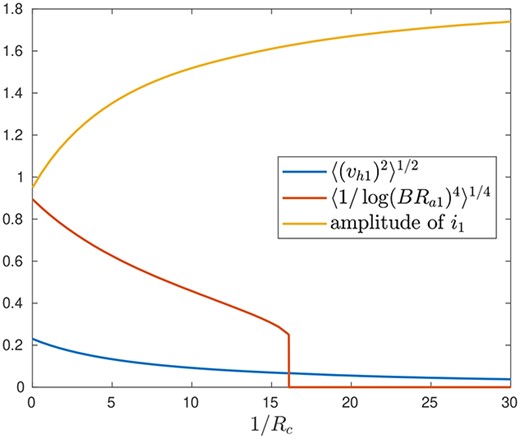
Fig. 11.

Plot of the time-averaged arc temperature $⟨ 1 / \log (B R_{a 1})^{4} ⟩^{1 / 4}$ ⁠, time-averaged hearth voltage $⟨ v_{h 1}^{2} ⟩^{1 / 2}$ and the amplitude of $i_{1}$ ⁠, as functions of the charge conductance $1 / R_{c}$ ⁠.

Open in new tab Download slide

as functions of the charge conductance $1 / R_{c}$ ⁠. We can interpret the terms in (4.1) as an average arc temperature, and root-mean-square (rms) voltage across the hearth region, respectively.

As in Luckins et al. (2021), we see that as the charge conductance increases, the rms voltage across the hearth decreases, and the average arc radiation also decreases, as less current passes through the arc, and more passes through the charge. For sufficiently large charge conductance, the only periodic solution of our model has $i_{a} = 0$ ⁠, so that all the current passes through the charge, and there is no heat radiated by the arc.

In Luckins et al. (2021), we prescribed the total current $i_{1}$ to be sinusoidal, with prescribed (constant) amplitude. With the full EC model, we instead solve for the total current $i_{1}$ as part of the solution of our model, and we see in Fig. 11 that the amplitude of the total current $i_{1}$ increases with the charge conductance. It is not clear what effect this might have on the solution of the homogenized model of Luckins et al. (2021) for the slow-evolution of the charge material, and this would be an interesting area for future investigation. We note that since we have used a different nondimensionalization, the values in Fig. 11 would need to be rescaled before use in the homogenized model of Luckins et al. (2021).

4.6 Asymmetric parameters

In all previous numerical solutions of this section we have restricted to the symmetric case, with all parameters equal in each of the three phases. This is the simplest case but it is not usually observed in practice: more often there is asymmetry in the electrical measurements from the three phases. In this section, we introduce asymmetry in some of the parameters, to observe the effect on the solution.

In practice, the furnace electrodes may be raised and lowered by the furnace operators in order to adjust the current distribution. We therefore investigate the effect of varying the arc length $h_{a}$ ⁠, so that phase 1 has a longer arc than the other two. In our dimensionless model, increasing $h_{a}$ corresponds to smaller $B_{1}$ and larger $p_{r 1}$ values for that phase. Solutions of (3.2) with (3.4a) for this asymmetric system are shown in Fig. 12a–b. We note that, as expected, the arc current $i_{a 1}$ and total current $i_{1}$ are lower than the other phases, since arc 1 is more resistive than the other arcs. This is also seen in the arc signature, which is very different for phase 1 than phases 2 and 3. Interestingly, the asymmetry does not seem to affect both the phase 2 and 3 currents equally: their arc signatures are very similar shapes, but the amplitude of the currents are different, with the maximum of phase 3 below the maximum of phase 2. This may be due to the inherent asymmetry of the electric arc component: arc 1 is more conductive in the parts of the AC cycle when the current magnitude is decreasing than when it is increasing, and so affects phases 2 and 3 in different ways.

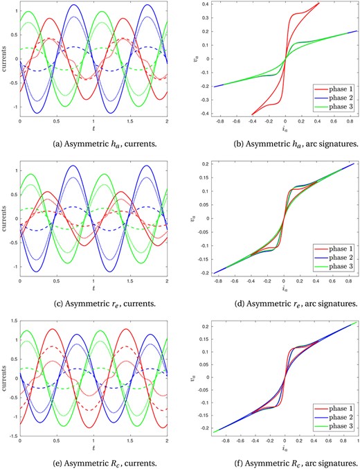
$Solutions with asymmetric parameters. In (a) and (b) the arc length $h_a$ of phase 1 is longer than phases 2 and 3, so that $B_1=4$, $B_2=B_3=12$, $p_{r1}=0.6$ and $p_{r2}=p_{r3}=0.2$. In (c) and (d), $r_{e1}=1$ for phase 1, but $r_{e2}=r_{e3}=0.18$. In(e) and (f), $R_{c1}=0.2$ for phase 1, but $R_{c2}=R_{c3}=1$. In (a), (c) and (e) we show the electrode currents (solid lines), arc currents (dotted lines) and charge currents (dashed lines) of each phase, with phase 1 in red, phase 2 in blue and phase 3 in green. In (b), (d) and (f) we show the corresponding arc signatures. Unless otherwise specified, we take the standard values $\zeta _r=8\times 10^{-3}$, $p_r=0.2$, $B=12$, $\zeta _I=0.13$, $r_{cr}=0.054$, $r_e=0.18$ and $R_c=1$.$

Fig. 12.

Solutions with asymmetric parameters. In (a) and (b) the arc length $h_{a}$ of phase 1 is longer than phases 2 and 3, so that $B_{1} = 4$ ⁠, $B_{2} = B_{3} = 12$ ⁠, $p_{r 1} = 0.6$ and $p_{r 2} = p_{r 3} = 0.2$ ⁠. In (c) and (d), $r_{e 1} = 1$ for phase 1, but $r_{e 2} = r_{e 3} = 0.18$ ⁠. In(e) and (f), $R_{c 1} = 0.2$ for phase 1, but $R_{c 2} = R_{c 3} = 1$ ⁠. In (a), (c) and (e) we show the electrode currents (solid lines), arc currents (dotted lines) and charge currents (dashed lines) of each phase, with phase 1 in red, phase 2 in blue and phase 3 in green. In (b), (d) and (f) we show the corresponding arc signatures. Unless otherwise specified, we take the standard values $ζ_{r} = 8 \times 10^{- 3}$ ⁠, $p_{r} = 0.2$ ⁠, $B = 12$ ⁠, $ζ_{I} = 0.13$ ⁠, $r_{c r} = 0.054$ ⁠, $r_{e} = 0.18$ and $R_{c} = 1$ ⁠.

Open in new tab Download slide

The electrodes in the furnace often have different lengths, and so different resistances. The base of the furnace, consisting of metal-rich carbon materials accumulated over time, may also not have uniform resistance in all three phases. We therefore now investigate the effect of varying the electrode/furnace base resistance $r_{e}$ ⁠, with solutions shown in Fig. 12c–d. Phase 1, with a much larger electrode resistance, has lower current passing through that phase than the other two, and both the arc and charge currents in that phase are also lower than in phases 2 and 3. Since the arc parameters are now the same in all phases, the arc signature plots have similar shape, although the current maximum is different for each phase. Again, the alteration to phase 1 does not affect phases 2 and 3 equally.

As discussed in Luckins et al. (2021), the resistance of the charge material depends on the local temperature and composition of the material. Finally, we therefore investigate the situation with phase 1 having much lower charge resistance $R_{c}$ ⁠, with solutions shown in Fig. 12e–f. We do not see such dramatic changes in the total current through each phase as in the previous asymmetric cases, and because the arc parameters are the same for each phase the arc signatures all have similar shape. However, phase 1 has significantly more current passing through the charge, and less through the arc, compared with the other two phases. Phases 2 and 3 are again affected differently, despite having the same parameters as each other.

5. Discussion

In this paper, we have incorporated the three-phase EC model of Valderhaug (1992) into the cell problem of the homogenized model of Luckins et al. (2021), which includes a radiation model for the electric arc. The resulting model consists of a system of five coupled ODEs for the phase currents and the resistances of the electric arcs. Since this work ties together two separate aspects of furnace modelling, the results of this paper may be viewed in different ways by each of these modelling communities.

Firstly, the EC model provides a much more accurate electrical description of the furnace for the homogenized model of Luckins et al. (2021). In Luckins et al. (2021) the total current $i_{1}$ was assumed to be sinusoidal, with prescribed amplitude. With the full EC model, we instead solve for the total current $i_{1}$ as part of the solution of our model. As discussed in Section 2.2.1, the time-averaged quantities (2.16) may be computed from the solution of the EC model, using the radiation arc model, in order to incorporate the EC model into the slow timescale model. We computed these quantities in Section 4.5, observing that the amplitude of the phase current $i_{1}$ increases with the charge conductance, rather than remaining constant as assumed in Luckins et al. (2021). It is not clear what effect this might have on solutions of the homogenized model of Luckins et al. (2021) for the slow-evolution of the charge material, and this would be an interesting area for future investigation.

Secondly, we may view the radiation arc model as an alternative to the semi-empirical Cassie or Mayr models (or the hybrids and additional empirical models used in the literature) in understanding the AC effects in the EC electrical system. We have compared the radiation model with the Cassie and Mayr models, by understanding each in terms of the conservation of energy in the arc, highlighting the different assumptions that are made about the dominant heat loss mechanisms, and the dependence of the heat content of the arc on the temperature or resistance of the arc. We observed from our numerical simulations that each arc model evolves within each AC half-period towards its steady-state current–voltage relationship (IV profile). The radiation arc model has a rising steady-state IV profile at the low arc resistances expected in a real furnace, compared with the constant-voltage profile for the Cassie model and the falling profile for the Mayr model. This provides some validation for the radiation model, since rising IV characteristics have been predicted by more sophisticated SAF arc models in the literature (Saevarsdóttir, 2002).

The radiation arc model has several advantages over the Cassie and Mayr models in addition to the rising IV characteristic. It is derived from first principles rather than semi-empirical, hence the model parameters have physical meaning and may be estimated from properties of the arc gases. The radiation model is also designed for SAF arcs (rather than for circuit-breaker arcs), taking into account the heat radiation which is known to be important for such high-current arcs. The radiation model is simple, with only one more parameter than either the Cassie or Mayr models, and allows for easy combination of the EC system with slow-timescale models for the heating, flow and chemical reactions in the charge.

We have explored the effect of varying the parameters in the radiation arc model. Increasing the arc length $h_{a}$ was seen to result in a lower arc current, and we found that there is a threshold arc length above which no arc forms at all, and all the current passes instead through the charge material. We have also investigated how the EC system (with the radiation arc model) is dependent on the parameters of the external electrical system, showing that the total current decreases with both increasing resistance in the electrode or furnace base, and with increasing inductance. Using physically derived arc parameters we observed reasonable agreement between our model and furnace data. We anticipate that incorporating additional physical mechanisms into an arc model, especially heat loss to convection, would improve further the fit between the model and data.

The numerical simulations in this paper were mostly restricted to the symmetric case, but in reality asymmetric measurements are much more commonly observed. Our asymmetric solutions for different arc-lengths, electrode/base resistances and charge resistances demonstrate that the asymmetric problem is very complicated, with phases 2 and 3 behaving differently, even though all the parameters for both those two phases were equal. Other parameters, including the resistance of the melt pool and the inductance in each phase, are also likely to be asymmetric in practice. Indeed, the phase parameters are not likely to be independent in reality, since the resistance of the charge material depends on its temperature, which is dependent on the averaged arc properties. More thorough investigation of the effect of asymmetrical parameter values is an important area for future work.

Our simulations give insight into how the solution of our model depends on the parameters of both the electric circuit and the arc-resistance model. Ideally, furnace operators would be able to solve the inverse problem, reconstructing the model parameters from the furnace measurements, and in this way infer the distribution of current in the furnace and understand how the arc is behaving. This inverse problem is likely to be very difficult to analyse as the furnace data that can easily be measured is limited to just the phase currents and voltages. The EC model—especially allowing for asymmetry between the phases—includes many parameters, so that it could easily be over-fit. For this reason it is especially important to ensure the sub-models are physical, and parameter values all fall within physically relevant ranges. Further investigation of how to approach this inverse problem is needed.

6. Conclusions

The radiation arc model presented in this paper gives a new, computationally inexpensive model for the arc resistance in an SAF. This model captures the key property of a rising IV characteristic, as predicted by more sophisticated arc models, but which is lacking in the commonly used empirical models. We have demonstrated how this radiation arc model may be included into an EC model for the furnace electrical system, solutions of which are simple and cheap to compute numerically. We have also shown how averaged results from this fast-timescale model (varying over the timescale of the alternating current) may be included into a homogenized model for the slower chemical processes inside an SAF. In this way, we have systematically connected the two bodies of furnace-modelling literature which each focus on only one of these timescales.

Acknowledgment

We would like to thank the anonymous referees for their constructive comments which improved the paper. In compliance with EPSRC’s open access initiative, the data in this paper is available from https://doi.org/10.5287/bodleian:KZE9JQ9Xd.

Funding

This publication is based on work supported by the EPSRC Centre For Doctoral Training in Industrially Focused Mathematical Modelling (EP/L015803/1) in collaboration with Elkem ASA.

References

Andresen

(

1995

)

Process model for carbothermic production of silicon metal

Master’s thesis

Norway

NTH

Google Scholar

Google Preview

OpenURL Placeholder Text

WorldCat

Awagan

G. R.

Thosar

A. G.

(

2016

)

Mathematical modeling of electric arc furnace to study the flicker

International Journal of Scientific & Engineering Research

684

–

695

Google Scholar

OpenURL Placeholder Text

WorldCat

Barker

I. J.

Rennie

M. S.

Hockaday

C. J.

Brereton-Stiles

P. J.

(

2007

) Measurement and control of arcing in a submerged-arc furnace.

The 11th International Ferroalloys Congress

. South Africa: Mintek.

Bhonsle

D. C.

Kelkar

R. B.

(

2014

) New time domain electric arc furnace model for power quality study.

2014 IEEE 6th India International Conference on Power Electronics (IICPE)

. United States, NY:

IEEE

, pp.

–

Google Scholar

Google Preview

OpenURL Placeholder Text

WorldCat

Bowman

Krüger

(

2009

)

Arc Furnace Physics

Düsseldorf

Verlag Stahleisen

Google Scholar

Google Preview

OpenURL Placeholder Text

WorldCat

Cassie

A. M.

(

1939

) Arc rupture and circuit severity: a new theory.

Conférence Internationale des Grands Réseaux Électriques à Haute Tension (CIGRE)

, Paris, France, vol.

102

, pp.

588

–

608

Golestani

Samet

(

2016

)

Generalised Cassie–Mayr electric arc furnace models

IET Generation, Transmission & Distribution

3364

–

3373

Google Scholar

Crossref

WorldCat

Gustavsson

(

2004

)

Evaluation and simulation of black-box arc models for high-voltage circuit-breakers

Master’s thesis

Norway

Institutionen för Systemteknik

Google Scholar

Google Preview

OpenURL Placeholder Text

WorldCat

Hannesson

T. H.

(

2016

)

The Si process drawings

Elkem Iceland

Google Scholar

Google Preview

OpenURL Placeholder Text

WorldCat

Logar

Dovžan

Škrjanc

(

2011

)

Mathematical modeling and experimental validation of an electric arc furnace

ISIJ International

382

–

391

Google Scholar

Crossref

WorldCat

Luckins

E. K.

Oliver

J. M.

Please

C. P.

Sloman

B. M.

Van Gorder

R. A.

(

2021

)

Homogenised model for the electrical current distribution within a submerged arc furnace for silicon production

European J. Appl. Math.

, pages

–

, https://doi.org/10.1017/S0956792521000243.

Google Scholar

OpenURL Placeholder Text

WorldCat

Mayr

(

1943a

)

Beiträge zur Theorie des statischen und des dynamischen Lichtbogens

Archiv für Elektrotechnik

588

–

608

Google Scholar

Crossref

WorldCat

Mayr

(

1943b

)

Über die Theorie des Lichtbogens und seiner Löschung

Elektrotechnische Zeitschrift

645

–

652

Google Scholar

OpenURL Placeholder Text

WorldCat

Parizad

Baghaee

H. R.

Tavakoli

Jamali

(

2009

) Optimization of arc models parameter using genetic algorithm.

2009 International Conference on Electric Power and Energy Conversion Systems, (EPECS)

. United States, NY:

IEEE

, pp.

–

Google Scholar

Google Preview

OpenURL Placeholder Text

WorldCat

Saevarsdóttir

(

2002

)

High current AC arcs in silicon and ferrosilicon furnaces

PhD thesis

Norway

NTNU

Google Scholar

Google Preview

OpenURL Placeholder Text

WorldCat

Schwarz

(

1971

)

Dynamisches verhalten eines gasbeblasenen turbulenzbestimmten Schaltlichtbogens

Elektrotechnische Zeitschrift-A

389

–

391

Google Scholar

OpenURL Placeholder Text

WorldCat

Shampine

L. F.

Reichelt

M. W.

(

1997

)

The MATLAB ODE suite

SIAM J. Sci. Comput.

–

Google Scholar

Crossref

WorldCat

Sloman

B. M.

Please

C. P.

Van Gorder

R. A.

Valderhaug

A. M.

Birkeland

R. G.

Wegge

(

2017

)

A heat and mass transfer model of a silicon pilot furnace

Metallurgical and Materials Transactions B

2664

–

2676

Google Scholar

Crossref

WorldCat

Sloman

B. M.

Please

C. P.

Van Gorder

R. A.

(

2018

)

Asymptotic analysis of a silicon furnace model

SIAM J. Appl. Math.

1174

–

1205

Google Scholar

Crossref

WorldCat

Sloman

B. M.

Please

C. P.

Van Gorder

R. A.

(

2020

)

Melting and dripping of a heated material with temperature-dependent viscosity in a thin vertical tube

J. Fluid Mech.

905

A16

Google Scholar

Crossref

WorldCat

Valderhaug

A. M.

(

1992

)

Modelling and control of submerged-arc ferrosilicon furnaces

PhD thesis

Norway

NTNU

Google Scholar

Google Preview

OpenURL Placeholder Text

WorldCat

Yuan

Sun

(

2013

)

Simulation of fault arc using conventional arc models

Energy and Power Engineering

Google Scholar

OpenURL Placeholder Text

WorldCat

This is an Open Access article distributed under the terms of the Creative Commons Attribution License (https://creativecommons.org/licenses/by/4.0/), which permits unrestricted reuse, distribution, and reproduction in any medium, provided the original work is properly cited.

Download all slides

Month:	Total Views:
July 2022	260
August 2022	308
September 2022	88
October 2022	73
November 2022	94
December 2022	77
January 2023	60
February 2023	69
March 2023	59
April 2023	40
May 2023	37
June 2023	27
July 2023	42
August 2023	38
September 2023	25
October 2023	19
November 2023	30
December 2023	26
January 2024	33
February 2024	41
March 2024	57
April 2024	29
May 2024	34
June 2024	50
July 2024	58
August 2024	39
September 2024	48
October 2024	23
November 2024	43
December 2024	28
January 2025	34
February 2025	53
March 2025	72
April 2025	40
May 2025	13

Article Contents

Modelling alternating current effects in a submerged arc furnace

Abstract

1. Introduction

2. Model statement

2.1 EC model

2.2 Modelling the arc resistance

2.2.1 Arc heat loss due to optically thin radiation

2.2.2 Commonly used models for the arc resistance

2.2.3 Discussion and comparison

2.3 Initial conditions

2.4 Industrial measurements

3. Nondimensionalization

4. Numerical solutions

4.1 The radiation arc model

4.2 Cassie and Mayr arc models

4.3 The circuit parameters

4.4 Comparison with furnace data

4.5 Time-averaged quantities for the homogenized model

4.6 Asymmetric parameters

5. Discussion

6. Conclusions

Acknowledgment

Funding

References

Citations

Views

Altmetric

Email alerts

Citing articles via

Latest

Most Read

Most Cited

Article Contents

Modelling alternating current effects in a submerged arc furnace

Abstract

1. Introduction

2. Model statement

2.1 EC model

2.2 Modelling the arc resistance

2.2.1 Arc heat loss due to optically thin radiation

2.2.2 Commonly used models for the arc resistance

2.2.3 Discussion and comparison

2.3 Initial conditions

2.4 Industrial measurements

3. Nondimensionalization

4. Numerical solutions

4.1 The radiation arc model

4.2 Cassie and Mayr arc models

4.3 The circuit parameters

4.4 Comparison with furnace data

4.5 Time-averaged quantities for the homogenized model

4.6 Asymmetric parameters

5. Discussion

6. Conclusions

Acknowledgment

Funding

References

Citations

Views

Altmetric

Email alerts

Citing articles via

Latest

Most Read

Most Cited

This Feature Is Available To Subscribers Only