


Abstract
Quantitative benchmarking is widely used in the industry to compare relative performance across a sample of organizations. A key analytical challenge lies in obtaining accurate measures of intrinsic organizational performance net of contextual or exogenous influences. In this paper, we propose a model-based adjustment approach for comparative benchmarking that allows the analyst to recover targeted metrics for specific aspects of innate performance. We outline the statistical theory underpinning our method, provide simulations to demonstrate its properties and describe practical examples for computation. The managerial relevance of the method is demonstrated via two real-world transport industry applications: adjusting for economies of scale and density in benchmarking average costs of urban metros and for service characteristics in benchmarking metro journey times.
1. Introduction
Quantitative benchmarking is widely used in industry to compare relative performance across a sample of organizations. Performance domains of interest range from strategic management functions to highly disaggregate activities (Francis & Holloway, 2007; Kaplan & Norton, 1992; Moriarty & Smallman, 2009). A typical quantitative benchmarking analysis involves computation of a set of metrics, sometimes referred to as key performance indicators (KPIs), using data observed on a sample of organizations. Deviation from the central tendency of a KPI is taken as an indicator of relative performance, and improvement targets are set for units that fall below defined threshold levels (Camp, 1989; Leibfried & McNair, 1992).
KPIs are useful in describing relative performance, for instance in the form of a performance ranking, but are typically of less value in explaining what lies behind the ranking itself. In particular, problems of interpretation can arise when benchmarking metrics do not readily partition the innate performance of organizations from other exogenous determinants. Under these conditions, KPIs can produce a somewhat obscured understanding of performance, or worse, can actually be highly misleading (Bogetoft, 2012). It is this well-known limitation of quantitative benchmarking that we aim to address in this paper.
To motivate our study, we begin by making a distinction between intrinsic and composite performance. By intrinsic performance, we mean the innate performance of organizations that the benchmarking analyst ultimately wants to measure and rank. Composite performance, on the other hand, is a combination of both intrinsic performance and of other exogenous determinants of performance that are not themselves of interest for benchmarking purposes. Such exogenous determinants could, for instance, include characteristics of the context or local environment in which an organization operates, but which are largely outside the control of the organization itself. In practice, it is often the case that available data allow us to benchmark composite performance but leave intrinsic performance unobserved. Our aim here is to describe an approach that can be used to recover a measure of intrinsic performance from observed data on composite performance.
To do so, we develop a simple model-based adjustment approach for comparative benchmarking. We achieve this by first removing ‘contamination’ from exogenous determinants via regression analysis and then by recovering adjusted performance metrics with reduced variance that are measured on the same scale as the original metric. Our adjusted benchmarking approach allows comparisons to be made on specially tailored definitions of performance and can generate useful insights through comparison of conditional and unconditional benchmarks.
The paper is structured as follows. Section 2 provides a brief review of relevant literature on efficiency measurement. Section 3 outlines our model-based approach for benchmarking. It first develops the basic statistical theory and then provides some practical examples for computation. Section 4 presents simulation results to demonstrate the properties of our proposed method. In Section 5 we demonstrate the managerial relevance of our approach through two real-world applications for the transport industry: one that adjusts for economies of scale and density in benchmarking average costs of urban metros and one that adjusts for service characteristics in benchmarking metro journey times. Conclusions are drawn in the final section.
2. Literature review
A wide range of quantitative methods may be adopted to evaluate and compare performance. The approaches most relevant to the work we develop in this paper are those concerned with efficiency frontier estimation, including stochastic frontier analysis (SFA) and data envelopment analysis (DEA) (Agrell & Bogetoft, 2017; Bogetoft, 2012).
Frontier techniques compare the efficiency of firms (or production entities) relative to a technological or production frontier. The frontier represents the maximum output attainable for a given level of inputs, and the position of the firms or units relative to the frontier indicates their relative efficiency. The SFA technique, first proposed by Aigner et al. (1977) and Meeusen & Broeck (1977), uses a parametric model to define the production frontier and includes terms that distinguish between efficiency and stochastic noise. The DEA method, introduced by Charnes et al. (1978), is non-parametric and consequently invokes less a priori assumptions to establish the production frontier, but typically does not explicitly model stochastic terms. Example applications of SFA and DEA include evaluating the efficiency of private firms or public agencies in finance (Tsolas, 2011), healthcare (Alexander et al., 2003), energy (Kuo, 2011; Tsolas, 2010) and transport (Canavan et al., 2015; Graham, 2008).
Exogenous determinants of productivity can be modelled using SFA and DEA approaches. For example, in SFA frameworks, exogenous determinants can be included as random and fixed effects terms or as latent variables as per Tsionas (2002), Greene (2005) and Schmidt et al. (2009). In DEA models, exogenous factors can be incorporated using one and two stage approaches (see Daraio & Simar, 2005, for further references) or through probabilistic conditional models as per Daraio & Simar (2005), Daraio & Simar (2007b) and Daraio & Simar (2007a).
However, while it is possible to distinguish between intrinsic and exogenous determinants of performance in frontier models, it is difficult to apply frontier techniques universally because in many cases performance cannot easily be conceptualized in an input–output-type formulation. In this paper, we propose a general model-based adjustment framework for conditional benchmarking, which to our knowledge is the first time such a formal framework has been set out.
3. Model-based adjustment for benchmarking
Throughout the paper we use the standard convention that upper case denotes random variables and lower case the realized values of random variables. The setting we address is one in which the full data for units under study would comprise realization of the random vector, |$Z_i=(Y_i,P_i,X_i)$|, |$i=(1,...,n)$|, where outcome variable |$Y_i$| is a composite performance metric for unit |$i$|, |$P_i$| is a vector of covariates that determine the intrinsic performance of unit |$i$| and |$X_i$| is a vector of covariates that capture measured exogenous influences on composite performance.
For the purposes of benchmarking we would like to reveal as much as possible about variation in intrinsic performance, which we denote |$Y_i(P_i)$|, but this quantity is not observed, and in fact even data on the vector |$P_i$| we also assume to be unavailable. Rather, we observe only |$Y_i$| and |$X_i$| and we are therefore left with no option but to benchmark performance using |$Y_i$|. To obtain a better understanding of intrinsic performance, our objective is to adjust |$Y_i$| to reduce the influence of exogenous factors |$X_i$|, and thus get closer to a measure of unobserved |$Y_i(P_i)$|. In addition, we want both our adjusted and unadjusted benchmarking metrics to be on the same scale to allow for direct comparison.
3.1 Statistical theory
However, the scenario we are interested in in this paper is one in which |$P_i$| is unobserved, or partially observed, so direct estimation of (1), and therefore of |$\theta _A$| and |$y_i(p_i)$|, is not possible. We do have a measure of composite performance in |$Y_i$|, but it is ‘contaminated’ by exogenous influences and therefore unsuitable as a measure of intrinsic performance. Our proposed solution is to use model-based adjustment to recover a more representative intrinsic performance metric. We will develop the theory under the assumption that exogenous influences |$X_i$| are independent of |$P_i$|, implying that |$X_i$| is a non-confounding vector. Later in the section we will discuss the implications that arise when this assumption fails.
In this way we can remove the effect of exogenous influences from our composite performance measure and return this adjusted metric to the original |$Y_i$| scale. The resulting quantity, |$\widehat{y}_i(p_i)$| has contamination from random noise, but not from exogenous influences and is thus a viable metric for intrinsic performance.
3.2 Practical calculations
To provide concrete examples of these calculations we derive them in the context of estimates obtained via linear and semiparameteric regression.
3.3 Dependence between |$P_i$| and |$X_i$|
When it is infeasible to assume that |$P_i$| ┴ |$X_i$|, and we do not observed |$P_i$|, then we face the problem of confounding and it is no longer possible to obtain consistent estimates of |$\beta $| from the marginal model (4). Such estimates will always be biased as long as |$P_i \not$| ┴ |$X_i$|.
Solutions to this problem can be found via application of methods for causal inference in the presence of unobserved confounders. A review of this material is outwith the scope of this article, but comprehensive descriptions of relevant estimators, including instrumental variables (IV), longitudinal random, fixed and dynamic methods, regression discontinuity designs (RDD) and difference-in-differences (DID), can be found in Diggle et al. (2002), Tsiatis (2006), Imbens & Wooldridge (2009), Imbens & Rubin (2015) Pearl et al. (2016) and Peters et al. (2017).
Whatever causal method is applied, the ultimate objective is to obtain consistent estimates of parameter vector |$\beta $| and follow the same procedure outlined above. Note that in situations for which causal inference is not possible, or is unlikely to produce appropriate estimates, recourse to the literature may provide statistical evidence that can be used to perform model-based adjustment and remove the effect of exogenous influences.
4. Simulations
Figure 1 shows a benchmarking comparison of ‘true’ composite and intrinsic performance for 30 units sampled from our simulated population. The simulated data of course provide exact values of intrinsic performance. In simulating our model, we want to test how well we can represent these values if they were unobserved, and instead we used our model-based method.
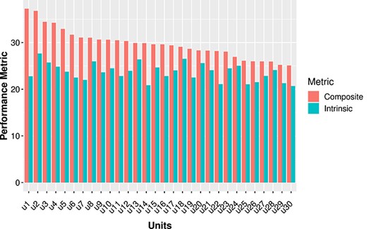
Comparison of composite and intrinsic performance metrics for simulated data.
Figure 1 shows that, if the objective is to reveal variance in intrinsic performance, then composite performance is not a particularly good metric to use. Composite performance is of course correlated with intrinsic performance, |$\rho _{P,Y} = 0.60$|, but because it also reflects exogenous influences it obscures the variance we wish to reveal and provides an incorrect ranking of units on |$P$|.
Simulation results for model-based adjusted benchmarking
| Truth | Est. | Var. | MSE | |
|---|---|---|---|---|
| |$\beta $| | 2.000 | 1.960 | 0.031 | 0.032 |
| |$\mu _Y$| | 30.000 | 30.063 | 0.130 | 0.134 |
| |$\mu _{Y(p)}$| | 30.000 | 30.063 | 0.130 | 0.134 |
| |$\sigma ^2_{Y}$| | 14.000 | 13.688 | 3.952 | 4.046 |
| |$\sigma ^2_{Y(p)}$| | 6.000 | 5.965 | 0.685 | 0.686 |
| |$\rho _{P,Y}$| | 0.598 | 0.589 | 0.004 | 0.004 |
| |$\rho _{P,Y(p)}$| | 0.913 | 0.908 | 0.000 | 0.000 |
Estimation of |$\beta $| is, as expected, unbiased and consistent because |$X$| and |$P$| are uncorrelated, and thus the marginal model with |$P$| omitted is correctly specified. The adjusted metric has the same simulated mean as the unadjusted metric, because as discussed above, it is on the same scale, but has smaller variance. This is because variance due to exogenous influences |$X$| has been removed. The mean simulated correlation coefficient between the unadjusted metric and intrinsic performance is 0.589, while the corresponding value for the adjusted metric is 0.913. This demonstrates that model-based adjustment leads to a substantial improvement in our ability to measure intrinsic performance.
5. Managerial relevance
In this section we apply the method outlined above to demonstrate its managerial relevance through two particular real-world benchmarking comparisons. First, using a unique dataset for 32 international metro operators collected annually by the Transport Strategy Centre (TSC) at Imperial College London, we adjust for the influence of metro size (e.g. scale economies) in benchmarking the average cost of urban metros. Second, using open data on passenger trips from the London Underground metro network, we adjust for service characteristics in benchmarking mean journey time performance across 22 origin-destination routes in Central London.
5.1 Adjusting for scale economies in benchmarking average costs
In this application our objective is to compare performance in cost efficiency across units, in this case metros, and to do this we construct a measure of the average cost of producing a metro car kilometre (e.g. the average cost of operating a single car of a metro train for a distance of one kilometre). Cost data for 2015 have been converted to international dollar equivalent using a purchasing power parity (PPP) currency converter published by the World Bank. The unadjusted benchmark is total operating cost per car kilometre. We find considerable variation in this unadjusted metric across systems, with a mean value of $5.76, a minimum of $3.04 and a maximum of $16.52. Thus, across our sample of urban metros we observe a fivefold difference in average cost with a variance of $6.21.
We know from the theoretical and empirical literature that the costs of urban metro operations are strongly influenced by the size of metro systems. A recent study by the TSC at Imperial College London finds evidence of considerable scale economies both from system size (measured by total route length in kms) and from the density of use of the system (measured by car kms operated per km of route length) (Anupriya et al., 2019). This study estimate an elasticity of average cost with respect to scale of 0.85 and with respect to density of 0.60. These results are consistent with economic theory and can be explained by the prevalence of fixed and quasi-fixed costs in metro operations.
Since there is typically little metros can do in the short run to make large-scale changes to system scale or density, it is informative to consider average costs that are adjusted for differences in scale and density. Essentially, this amounts to asking the following question: if we remove the influence of scale and density from our measure of composite performance (e.g. nullify the effect of two known strong exogenous influences on performance) how will this change the distribution of our cost performance metric for metros? Other things being equal, since there are positive scale and density effects, we would expect the adjusted metric to reduce the relative cost performance of large and densely used systems since they benefit most from these two exogenous influences.
To adjust for differences in scale and density, we apply the model-based adjustment method outlined above using the parameter values from Anupriya et al. (2019). A comparison of adjusted and unadjusted average cost metrics is shown in Fig. 2.
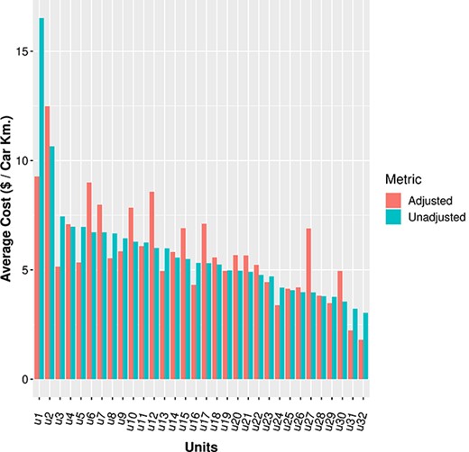
Unadjusted and adjusted average cost metrics for metro operators.
Two aspects of this comparison are worth emphasizing. First, by removing scale effects the variance in average cost is reduced from $6.21 to $4.71, thus demonstrating the considerable influence of scale on the unadjusted performance metric. Substantively, this suggest a priori that larger metros and metros with higher densities of traffic will tend to have lower average costs, ceteris paribus. Second, the figure shows that performance rankings are radically altered through adjustment.
From a managerial perspective, adjustment for scale and density is relevant for two reasons. First, since metro operators typically do not make large shifts in operational scale in the short run, the influence of scale on performance is largely not actionable, and therefore arguably should not be something we incorporate in a benchmark used to target performance improvements. Second, the revised performance ranking based on the conditional benchmark gives managers a much better undertaking of how well their organization is doing, net of scale effects, and thus a more realistic picture of where they sit within the industry.
5.2 Adjusting for service characteristics in benchmarking metro journey times
In the second application of our model-based adjustment method, the objective is to quantify journey time performance by comparing mean journey times on a sample of the busiest routes on the Central, Jubilee and Victoria lines of the London Underground metro network. Data on passenger journey times are obtained from the Transport for London (TfL) open source data repository, and cover 2 weeks in October in 2015 (Transport for London, 2015). Average journey times are recorded for each unit, in this case an origin–destination route, for each half hour period per day, and a sample of 22 of the busiest origin–destination routes within central London are analysed. Unadjusted benchmarks are calculated at a route level as the mean journey time in minutes across all trips undertaken on the route over the 2-week time period. The unadjusted mean journey times range from a minimum of 5.61 mins to a maximum of 17.17 mins. Across all routes, the mean value of unadjusted mean journey times is 12.10 mins and the variance is 11.07 mins|$^2$|.
Comparing mean journey times across routes does not in itself provide useful information, since the values primarily represent differences in route length and operating conditions. In their analysis of metro journey times on the London Underground, Singh et al. (2020) demonstrated that along with route length, operational characteristics such as train frequency and congestion from passenger demand have the most influential impact on passenger journey times. In assessing journey time performance, it is of interest for operators to understand whether there are inherent differences across routes that may not be within operator control after conditioning for known operational characteristics. We therefore apply the model-based adjustment method to compute adjusted mean journey times conditioning for route length, train frequency and passenger flows. The data on passenger route flows per half hour per day are obtained from the same 2015 TfL open data set on journey times (Transport for London, 2015). Open data on average train frequencies are only available for 2018 (Transport for London, 2018) and these data are considered appropriate to approximate operating frequencies in 2015 for use in the model. Data on route lengths are publicly available from Transport for London (2008). Figure 3 illustrates the resulting adjusted and unadjusted journey time benchmarks.
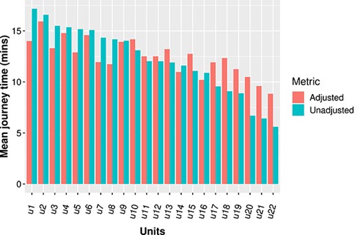
Unadjusted and adjusted mean journey time metric for sample of routes on London Underground.
In the adjusted model, route-specific effects are significant at a level of 95% (|$\alpha $|=0.05), indicating that routes do possess inherent characteristics that create prevailing differences in journey time performance over and above sources of variance from known service characteristics. As with the previous example, the adjusted benchmarks yield a different ranking of routes compared to the unadjusted benchmarks. The variance across rankings reduces from 11.07 mins|$^2$| for the unadjusted benchmarks to 3.14 mins|$^2$| for the adjusted benchmarks.
Model-based adjusted benchmarking is potentially informative to metro operators in this case, because in showing that the operational factors included in the adjusted model plausibly capture the majority of variance in journey times, it indicates where else operators can best focus their efforts to improve journey time performance.
6. Conclusions
In this paper we have proposed a model-based approach for comparative benchmarking that adjusts for exogenous determinants of performance to produce more targeted benchmarking metrics. We have described the statistical theory underpinning our approach and proposed some example calculations for computation. Simulations have demonstrated the properties of our model-based adjustment approach showing that it performs well in removing ‘contamination’ through variance reduction via marginalization. The managerial relevance of the method is demonstrated via two real-world transport industry applications: adjusting for economies of scale and density in benchmarking average costs of urban metros and for service characteristics in benchmarking metro journey times.
Model-based adjusted benchmarking can help managers recover more focused measures of performance that they can then target for improvement and best practice. It also allows them to compare conditional and unconditional benchmarks, which can be illuminating in identifying areas for further investigation.
References


