


Abstract
The analysis of an |$\textbf {H}(\textrm {div})$|-conforming method for a model of double-diffusive flow in porous media introduced in Bürger, Méndez & Ruiz-Baier (2019, On H(div)-conforming methods for double-diffusion equations in porous media. SIAM J. Numer. Anal., 57,1318–1343) is extended to the time-dependent case. In addition, the efficiency and reliability of residual-based a posteriori error estimators for the steady, semidiscrete and fully discrete problems are established. The resulting methods are applied to simulate the sedimentation of small particles in salinity-driven flows. The method consists of Brezzi–Douglas–Marini approximations for velocity and compatible piecewise discontinuous pressures, whereas Lagrangian elements are used for concentration and salinity distribution. Numerical tests confirm the properties of the proposed family of schemes and of the adaptive strategy guided by the a posteriori error indicators.
1. Introduction and problem formulation
1.1 Scope
A number of physical problems of relevance in industrial applications involve coupled incompressible flow and double-diffusion transport. We are interested in numerical schemes for the approximation of a class of coupled equations that arise as models of sedimentation of small particles under the effect of salinity of the ambient fluid. The governing model can be stated as follows (cf., e.g., Burns & Meiburg, 2015; Reali et al., 2017):
posed on a spatial domain |$\varOmega \subset \mathbb {R}^d$|, |$d=2$| or |$d=3$|, where |$t\in (0,t_{\textrm {end}}]$| is time, |$\boldsymbol {u}$| is the fluid velocity, |$\nu $| is the concentration-dependent viscosity, |$\rho _{\textrm {m}}$| is the mean density of the fluid, |$p$| is pressure, |$\rho $| is density, |$\boldsymbol {g}$| is the gravity acceleration, |$s$| is the salinity concentration and |$c$| is the concentration of solid particles. These equations state momentum (1.1a), mass (1.1b) conservation of the fluid and transport of the species (1.1c)–(1.1d). The Schmidt number |$\textrm {Sc} = \nu _{\textrm {ref}} / \kappa _{\textrm {s}}$| is the ratio between kinematic viscosity and diffusivity (here assumed relatively small, e.g., |$\textrm {Sc} = \mathcal {O}(10)$|, so that concentration and salinity boundary layers are fully resolved; see, e.g., Kadoch et al., 2012; Rasthofer & Gravemeier, 2018), where |$\kappa _{\textrm {s}}$| is the diffusivity of salinity, and |$\nu _{\textrm {ref}}$| is a reference viscosity in the absence of solid particles. Finally, |$\tau = \kappa _{\textrm {s}} / \kappa _{\textrm {c}}$| is the inverse of the diffusivity ratio, where |$\kappa _{\textrm {c}}$| is the diffusivity of solid particles, and |$\boldsymbol {e}_z$| is the upward-pointing unit vector. We relate the densities through a linearized equation of state
where |$\alpha $| and |$\beta $| are model constants that approximate the derivatives of the equation of state. Again, as in the works by Burns & Meiburg (2015); Ruiz-Baier & Lunati (2016); Reali et al. (2017), the solid particles are assumed to be mono-sized with radius |$r$|, and they settle at dimensionless velocity |${v_{\textrm {p}} =\frac { v_{\textrm {St}}} {( \nu _{\textrm {ref}} g^{\prime})^{1/3}}}$|, where |${v_{\textrm {St}} = \frac {2 r^2 ( \rho _{\textrm {p}} - \rho _{\textrm {m}})g}{9 \rho _{\textrm {m}} \nu _{\textrm {ref}}}}$| is the Stokes velocity (settling velocity of a single particle in an unbounded fluid). The coupling mechanisms between flow and transport are only due to advection for concentration and salinity (where the advecting velocity for concentration, |$\textbf {u} - v_{\textrm {p}}\textbf {e}_z$|, is also divergence-free), and through the concentration-dependent viscosity. Further details (including boundary and initial conditions) are provided in later parts of the paper.
To put the paper further into the proper perspective, we mention that there exists an abundant body of literature devoted to constructing accurate finite element and related schemes for double-diffusive flows. Some recent contributions include variational multiscale stabilized schemes, least-squares methods, divergence-conforming mixed methods, volume-averaging discretizations, spectral elements, vorticity-based finite element formulations and similar methods applied to, e.g., flows with heat and mass transport (Abedi & Aliabadi, 2003), reactive Boussinesq flows (Agouzal & Allali, 2003), nonlinear advection–reaction–diffusion in the context of bioconvective flows (Lenarda et al., 2017; Anaya et al., 2018), cross-diffusion and boundary layer effects in double-diffusive Navier–Stokes–Brinkman equations (Dallmann & Arndt, 2016; Bürger et al., 2019; Baird et al., 2021) and in Darcy–Brinkman equations (Yang & Jiang, 2018), or phase change models (Zabaras & Samanta, 2004; Danaila et al., 2014; Zimmerman & Kowalski, 2017; Woodfield et al., 2019); where the list is far from exhaustive.
The solvability analysis for the continuous and discrete problems usually follows energy and fixed-point schemes as done for classical Boussinesq equations, and this is also the approach we follow here. The discretization in space uses an interior penalty divergence-conforming method for the flow equations (in this case, Brezzi–Douglas–Marini (BDM) elements of degree |$k\geq 1$| for the velocity and discontinuous elements of degree |$k-1$| for the pressure following Arnold et al., 2002; Könnö & Stenberg, 2011), combined with Lagrangian elements for the diffusive quantities. The present formulation and its analysis stand as a natural extension of the formulation in Bürger et al. (2019) to the transient case. As such, the proposed method also features exactly divergence-free velocity approximations ensuring local conservativity, and the error estimates of velocity are pressure-robust. The chosen time discretization is the backward differentiation formula of degree 2 (BDF2), which for |$k=2$| gives a method of order 2 in space and time. Existence of discrete solutions is established by the Brouwer fixed-point theory similarly as in Bürger et al. (2019), and the error analysis in the semidiscrete and fully discrete settings is adapted from the theory of Aldbaissy et al. (2018) for the Boussinesq equations and that of Baird et al. (2021) for filtration in axisymmetric domains.
In many applications where double-diffusion effects occur, complicated flow patterns exist in zones far from boundary layers and sufficiently refined meshes are needed essentially in the whole spatial domain. However, for salinity-driven settling of solid particles that result in mathematical models such as (1.1), many of the flow features are clustered near zones of high gradients of concentration, which is where the typical plumes are observed (Burns & Meiburg, 2015; Lenarda et al., 2017). This motivates the use of adaptive mesh refinement guided by a posteriori error indicators. For instance, in the context of phase change models, there are some results based on error-related metric change (Danaila et al., 2014; Rakotondrandisa et al., 2020) and on goal-oriented adaptivity (Zimmerman & Kowalski, 2017). Regarding the design and rigorous analysis of residual-based a posteriori error estimators for flow-transport couplings, the literature is predominantly focused on the stationary case (see, e.g., Becker & Braack, 2002; Allali, 2005; Zhang et al., 2011; Alvarez et al., 2016; Agroum, 2017; Alvarez et al., 2018; Dib et al., 2019; Wilfrid, 2019; Allendes et al., 2020 and the references therein). Only a few results are available for the time-dependent regime, from which we mention the adaptive mixed method for Richards equation in porous media (Bernardi et al., 2014), the remeshing scheme based on goal-oriented adaptivity for solidification problems advanced in Belhamadia et al. (2019), the collection of adaptive schemes for reactive flow discussed in Braack & Richter (2007) and for heat transfer in Larson et al. (2008). However, none of these theoretical frameworks directly handles divergence-conforming approximations to (1.1).
The a posteriori error analysis we advance here is of residual type, and its analysis uses ideas from the abstract results related to spatial estimators for discontinuous Galerkin schemes applied to parabolic problems in Georgoulis et al. (2011). The approach hinges on a decomposition of the discrete solution into a conforming and a nonconforming contribution, along with a reconstruction technique (see also Memon et al., 2012). This has also been exploited for the construction of a posteriori estimators of time-dependent Stokes and Navier–Stokes equations (Zhang & Li, 2017; Bänsch & Brenner, 2019). Our a posteriori error analysis is divided into three parts. In the first part, we present the error estimator for the steady coupled problem, under the assumption of |$\textbf {L}^2$| distributed force and constant source terms. In the second part, we extend the a posteriori error estimation to the semidiscrete method, and finally we present the a posteriori error estimator for the unsteady coupled problem. For the sake of simplicity, we restrict the latter part of the analysis to the backward Euler method. To the best of our knowledge, the a posteriori error estimation advanced herein is the first comprehensive study targeted for transient double-diffusive flows.
1.2 Outline
The remainder of this paper is organized as follows. In what is left of this section, we outline the weak formulation of (1.1), state preliminary results and notation to be used in throughout the manuscript and announce the stability of the continuous problem. In Section 2, we introduce the divergence-conforming method in fully discrete form, show existence of discrete solutions using fixed-point arguments and rigorously establish a priori error estimates. Section 3 is devoted to the construction and analysis of efficiency and reliability for a residual-based a posteriori error estimator tailored for the stationary problem. In turn, these upper and lower bounds are used to establish properties of a second family of estimators for the transient case, and addressed in Sections 4 and 5. In Section 6, we collect numerical tests that verify the theoretical convergence rates predicted by the a priori error analysis, confirm the robustness of the proposed a posteriori error estimators and illustrate the use of adaptive methods in the simulation of double-diffusive flows.
1.3 Preliminaries
Let |$\varOmega $| be an open and bounded domain in |$\mathbb {R}^{d}$|, |$d=2,3$| with Lipschitz boundary |$\varGamma =\partial \varOmega $|. We denote by |$L^p(\varOmega )$| and |$W^{r,p}(\varOmega )$| the usual Lebesgue and Sobolev spaces with respective norms |$\smash {\left \|\cdot \right \|_{L^p(\varOmega )}}$| and |$\smash {\left \|\cdot \right \|_{W^{r,p}(\varOmega )}}$|. If |$p=2$|, we write |$H^r(\varOmega )$| in place of |$\smash {W^{r,p}(\varOmega )}$| and denote the corresponding norm by |$\smash {\left \|\cdot \right \|_{r,\varOmega }}$| (|$\smash {\left \|\cdot \right \|_{0,\varOmega }}$| for |$H^0(\varOmega ) = L^2(\varOmega )$|). The space |$L^2_0(\varOmega )$| denotes the restriction of |$L^2(\varOmega )$| to functions with zero mean value over |$\varOmega $|. For |$r\geq 0$|, we write the |$H^r$|-seminorm as |$\smash {\left |\cdot \right |{{}}_{r,\varOmega }}$| and we denote by |$(\cdot ,\cdot )_{\varOmega }$| the usual inner product in |$L^2(\varOmega )$|. Spaces of vector-valued functions (in dimension |$d$|) are denoted in bold face, i.e., |$\smash {\textbf {H}^r(\varOmega ) = \left [ H^r(\varOmega ) \right ]^{d}}$|, and we use the vector-valued Hilbert spaces
where |$\textbf {n}_{\partial \varOmega }$| denotes the outward normal on |$\partial \varOmega $|; and we endow these spaces with the norm |$\left \|\cdot \right \|_{\operatorname *{div},\varOmega }$| defined by |$\smash {\left \|\textbf {w}\right \|_{\operatorname *{div},\varOmega }^2 := \left \|\textbf {w}\right \|_{0,\varOmega }^2 + \left \|\operatorname *{div} \textbf {w}\right \|_{0,\varOmega }^2}$|. We denote by |$L^s(0,t_{\textrm {end}};W^{m,p}(\varOmega ))$| the Banach space of all |$L^s$|-integrable functions from |$[0,t_{\textrm {end}}]$| into |$W^{m,p}(\varOmega )$|, with norm
1.4 Additional assumptions and weak formulation
As in, e.g., Dib et al. (2019), we assume that viscosity is a Lipschitz continuous and uniformly bounded function of concentration, i.e.,
for any |$c,c_1,c_2\in \mathbb {R}$|, and where |$L_{\nu },\nu _1,\nu _2$| are positive constants.
For simplicity of notation in presenting the analysis, we restrict the weak form to the case of homogeneous Dirichlet boundary conditions for velocity, concentration and salinity:
Let us define the following spaces:
For ease of the subsequent presentation, as in Schroeder et al. (2018), velocity, pressure, concentration and salinity solutions will be assumed to belong to the spaces |$\textbf {V}^t$|, |$Q^t$|, |$M^t$| and |$M^t$|, respectively. Testing each equation in problem (1.1) against suitable functions and integrating by parts whenever adequate gives the following weak formulation: find |$(\textbf {u},p,s,c) \in {\textbf {V}^t\times Q^t \times M^t \times M^t}$| such that |$\textbf {u}(\cdot ,0)=\textbf {u}_0 \in \textbf {H}_0(\operatorname *{div}\!^0;\varOmega )$|, |$s(\cdot ,0)=0$|, |$c(\cdot ,0)=0$| in |$\varOmega $| and for a.e. |$t \in [0, t_{\textrm {end}}]$|,
where the variational forms |$a_1: H_0^1(\varOmega )\times \textbf {H}_0^1(\varOmega )\times \textbf {H}_0^1(\varOmega )\to \mathbb {R}$|, |$a_2: H_0^1(\varOmega )\times H_0^1(\varOmega ) \to \mathbb {R}$|, |$b: \textbf {H}_0^1(\varOmega )\times L_0^2(\varOmega )\to \mathbb {R}$|, |$c_1: \textbf {H}_0^1(\varOmega )\times \textbf {H}_0^1(\varOmega )\times \textbf {H}_0^1(\varOmega )\to \mathbb {R}$|, |$c_2: \textbf {H}_0^1(\varOmega )\times H_0^1(\varOmega )\times H_0^1(\varOmega )\to \mathbb {R}$|, |$F:\textbf {H}^1_0(\varOmega ){\times H_0^1(\varOmega )\times H_0^1(\varOmega )}\to \mathbb {R}$| are defined as follows for all |$\textbf {u},\textbf {v},\textbf {w}\in \textbf {H}_0^1(\varOmega )$|, |$q\in L_0^2(\varOmega )$| and |$\varphi ,\psi \in H_0^1(\varOmega )$|:
1.5 Stability of the continuous problem
We begin by noting that the variational forms defined above are continuous for all |$\textbf {u},\textbf {v},\in \smash {\textbf {H}^1_0}(\varOmega )$|, |$q\in L^2_0(\varOmega )$| and |$\varphi ,\psi \in \smash {H^1_0}(\varOmega )$|:
We also recall (from Girault et al., 2005, Chapter I, Lemma 3.1, for instance) the following Poincaré–Friedrichs inequality:
Next, inequality (1.4) readily gives the coercivity of |$a_2$| and also, for a fixed concentration, that of |$a_1$|, i.e., there exist positive constants |$\alpha _a$| and |$\hat {\alpha }_a$| such that
Using the definition and characterization of the kernel of the bilinear form |$b(\cdot ,\cdot )$|, we can write
and applying integration by parts we can readily observe that
It is well known that the bilinear form |$b(\cdot ,\cdot )$| satisfies the inf-sup condition (see, e.g., Temam, 2001):
Finally, for |$\textbf {v} \in \textbf {W}^{1,\infty }(\varOmega )$| and |$\varphi \in W^{1,\infty }(\varOmega )$|, one can show that there exists an embedding constant |$C_{\infty }> 0 $| such that
A problem similar to (1.2) was studied by Agroum et al. (2015). Assuming that |$F\in L^2(0,t_{\textrm {end}}; \textbf {H}^{-1}(\varOmega ))$|, that the initial velocity |$\textbf {u}_0$| belongs to |$\textbf {L}^2(\varOmega )$| and that the initial data for the coupled species (|$s$| and |$c$| in our context) belong to |$L^2(\varOmega )$|, the authors showed existence of a solution by using the Galerkin method and applying the Cauchy–Lipschitz theorem and proved its uniqueness in two dimensions. Such analysis can be applied to (1.2) by noting that |$F$| is a Lipschitz-continuous function of |$c$| and |$s$|, and assuming the initial data belong to appropriate spaces. This is, however, not the focus of the paper and, instead, we move on to the discrete analysis.
2. Finite element discretization and a priori error bounds
2.1 Preliminaries
We discretize in space by a family of regular partitions, denoted |${\mathcal {T}}_h$|, of |$\varOmega \subset \mathbb {R}^d$| into simplices |$K$| (triangles in 2D or tetrahedra in 3D) of diameter |$h_K$|. We label by |$K^-$| and |$K^+$| the two elements adjacent to a facet (an edge in 2D or a face in 3D), while |$h_e$| stands for the maximum diameter of the facet. Let |${\mathcal {E}}_h$| denote the set of all facets and |$\smash {{\mathcal {E}}_h = {\mathcal {E}}_h^i \cup {\mathcal {E}}_h^{\partial }}$| where |${\mathcal {E}}_h^i$| and |${\mathcal {E}}_h^{\partial }$| are the subset of interior facets and boundary facets, respectively. If |$\textbf {v}$| and |$w$| are smooth vector and scalar fields defined on |${\mathcal {T}}_h$|, then (|$\textbf {v}^\pm , w^\pm $|) denote the traces of (|$\textbf {v},w$|) on |$e$| that are the extensions from the interior of |$K^+$| and |$K^-$|, respectively. Let |$\textbf {n}^+_e$|, |$\textbf {n}^-_e$| be the outward unit normal vectors on the boundaries of two neighbouring elements sharing the facet |$e$|, |$K^+$| and |$K^-$|, respectively. We also use the notation |$(\textbf {w}_e\cdot \textbf {n}_e)|_{e}=(\textbf {w}^{+}\cdot \textbf {n}^{+}_e)|_{e}$|. The average |$ {\cdot }$| and jump |$\left [\!\left [{\cdot } \right ]\!\right ]$| operators are defined as
whereas for boundary jumps and averages we adopt the conventions |$ \{\!\{{\textbf {v}}\}\!\} = \left [\!\left [\textbf {v}\right ]\!\right ] = \textbf {v}$|, and |$ \{\!\{{w}\}\!\} = \left [\!\left [w\right ]\!\right ] = w$|. In addition, |$\nabla _h$| will denote the broken gradient operator.
2.2 Galerkin method
For |$k\geq 1$| and a mesh |${\mathcal {T}}_h$| on |$\varOmega $|, let us consider the discrete spaces (see e.g., Brezzi et al., 1985)
which, in particular, satisfy |$\operatorname *{div}\textbf {V}_h\subset \mathcal {Q}_h$| (cf. Könnö & Stenberg, 2011). Here |${\mathcal {P}}_k(K)$| denotes the local space spanned by polynomials of degree up to |$k$| and |$\textbf {V}_h$| is the space of divergence-conforming BDM elements. Associated with these finite-dimensional spaces, we state the following semidiscrete Galerkin formulation for problem (1.2): find |$(\textbf {u}_h, p_h, s_h,c_h) \in \textbf {V}_h^t\times \mathcal {Q}_h^t\times \mathcal {M}_{h,0}^t\times \mathcal {M}_{h,0}^t$| such that:
The discrete versions of the variational forms |$a_1^h(\cdot ;\cdot ,\cdot )$| and |$c_1^h(\cdot ;\cdot ,\cdot )$| are defined using a symmetric interior penalty and an upwind approach, respectively (see, e.g., Arnold et al., 2002; Könnö & Stenberg, 2011):
where |$a_0>0$| is a jump penalization parameter.
We partition the interval |$[0,t_{\textrm {end}}]$| into |$N$| subintervals |$[t_{n-1},t_n]$| of length |$\varDelta t$|. We use the implicit BDF2 scheme where all first-order time derivatives are approximated using the centred operator
(similarly for |$\partial _t c$|) and for the first time step a first-order backward Euler method is used from |$t^0$| to |$t^1$|, starting from the interpolates |$\textbf {u}_h^0, s_h^0$| of the initial data:
In what follows, we define the difference operator
for any quantity indexed by the time step |$n$|. For instance, (2.3) can be written as |$\partial _t \textbf {u}_h (t^{n+1})\approx \frac {1}{2 \varDelta t} \mathcal {D} \boldsymbol {u}_h^{n+1}$|.
The resulting set of nonlinear equations is solved by an iterative Newton–Raphson method with exact Jacobian. Hence for |$1 \leq n \leq N-1$|, the complete discrete system is given by
2.3 Properties of the discrete problem
For the subsequent analysis, we introduce for |$r \geq 0$| the broken |$\textbf {H}^r$| space
as well as the mesh-dependent broken norms
where the stronger norm |$\smash {\left \|\cdot \right \|_{2,{\mathcal {T}}_h}}$| is used to show continuity. By using the inverse estimate
it can be seen that this norm is equivalent to |$\smash {\left \|\cdot \right \|_{1,{\mathcal {T}}_h}}$| on |$\textbf {V}_h$| (see, e.g., Arnold et al., 2002). We also define the discrete kernel of the bilinear form |$b(\cdot ,\cdot )$| as
Finally, adapting the argument used in Karakashian & Jureidini (1998, Proposition 4.5), we can state the following version of the discrete Sobolev embedding: for |$r=2,4$| there exists a constant |$C_{\textrm {emb}}>0$| such that
With these norms, we can establish continuity of the trilinear and bilinear forms constituting the variational formulation. The proof follows from Arnold et al. (2002, Section 4).
where the constant |$\smash {\tilde {C}_{\textrm {Lip}}>0}$| is independent of |$h$| (cf. Bürger et al., 2019). Note that while the coercivity of the form |$a_2(\cdot ,\cdot )$| in the discrete setting is readily implied by (1.5b), there also holds (cf. Könnö & Stenberg, 2011, Lemma 3.2)
provided that the stabilization parameter |$a_0>0$| in (2.2a) is sufficiently large and independent of the mesh size.
Let |$\textbf {w} \in \textbf {H}_0(\operatorname *{div}^0;\varOmega )$|, and let us introduce the jump seminorm
Then, due to the skew-symmetric form of the operators |$c_1^h$| and |$c_2$|, and the positivity of the nonlinear upwind term of |$c_1^h$|, we can write
as well as the following relation (which is based on (2.7) and follows by the same method as in Karakashian & Jureidini, 1998): for any |$\textbf {w}_1,\textbf {w}_2, \textbf {u} \in \textbf {H}^2({\mathcal {T}}_h)$|, there holds
We also have
Finally, we recall from Könnö & Stenberg (2011) the following discrete inf-sup condition for |$b(\cdot ,\cdot )$|, where |$\tilde {\beta }$| is independent of |$h$|:
2.4 Stability
As an auxiliary technical tool, we will also require the following algebraic relation: for any real numbers |$a^{n+1}$|, |$a^n$|, |$a^{n-1}$| and defining |$\varLambda a^n := a^{n+1} - 2a^n + a^{n-1}$|, we have
Note that, in contrast to the linear case, the stability result and the existence of a discrete solution do not guarantee, in general, uniqueness of solution.
2.5 Solvability
Let |$H$| be a finite-dimensional Hilbert space with scalar product |$(\cdot ,\cdot )_H$| and corresponding norm |$\left \|\cdot \right \|_H$|. Let |$\varPhi \colon H \to H$| be a continuous mapping for which there exists |$\mu> 0$| such that |$(\varPhi (u),u)_H \geq 0$| for all |$u \in H$| with |$\left \|{u}\right \|_H = \mu $|. Then there exists |$u \in H$| such that |$\varPhi (u) = 0$| and |$\left \|{u}\right \|_H \leq \mu $|.
2.6 A priori error estimates
The analysis in this section follows from standard arguments applicable to the approximation and error bounds for isolated solutions. For this, we require to assume the uniqueness of discrete solution.
Let us denote by |${\mathcal {I}}_h\,\colon {H^2(\varOmega )} \to \mathcal {M}_h$| the nodal interpolator with respect to a unisolvent set of Lagrangian interpolation nodes associated with |$\mathcal {M}_h$|. Furthermore, |$\varPi _h\, \textbf {u}$| denotes the BDM projection of |$\textbf {u}$|, and |${\mathcal {L}}_h\, p$| is the |$L^2$|-projection of |$p$| onto |$\mathcal {Q}_h$|. Under usual assumptions, the following approximation properties hold (see Könnö & Stenberg, 2011):
The following development follows the structure adopted in Aldbaissy et al. (2018). We begin with a property of the discrete bilinear forms and the continuous variational formulation.
Since we have assumed that |$\textbf {u}\in \textbf {H}^2(\varOmega )$|, integration by parts yields the required result. See also Arnold et al. (2002). The third and fourth equations are a straightforward consequence of properties of the continuous weak form.
Since for the following theorems we will assume the exact |$c$| and |$s$| belong to |$H^2(\varOmega )$|, we have |$c$|, |$s$||$\in C(\bar {\varOmega })$|. Now we decompose the errors as follows:
Assuming that |$\textbf {u}_h^0 = \varPi _h\, \textbf {u}(0)$|, |$s_h^0 = {\mathcal {I}}_h\, s(0)$| and |$c_h^0 = {\mathcal {I}}_h\, c(0)$|, we also use the notation |$E_{\textbf {u}}^n = (\textbf {u}(t_n) - \varPi _h\, \textbf {u}(t_n))$| and |$\xi _{\textbf {u}}^n = (\varPi _h\, \textbf {u}(t_n) - \textbf {u}_h^n)$|, and similar notation for other variables. Since for the first time iteration of system (2.1) we adopt a backward Euler scheme, a dedicated error estimate is required for this step.
For simplicity of notation, in what follows, we write down |$\textbf {u}^{\prime }$| instead of |${\partial _t \textbf {u}}$|, |$\textbf {u}^{\prime \prime }$| instead of |$\partial _{tt} \textbf {u}$|, and so on.
Note that, differently from the robust error analysis in, e.g., Han & Hou (2021) or in Schroeder et al. (2018), Theorems 2.6 and 2.7 require a smallness assumption on the velocity solution of the continuous problem. The assumption is needed due to the coupling through the viscosity with the balance equation of concentration. If such dependency is removed, for instance when a constant viscosity value is used, the smallness assumption is no longer required.
We next proceed to derive and analyse a posteriori error estimators. We split the presentation into three cases of increasing complexity, starting with an estimator focusing on the steady coupled problem.
3. A posteriori error estimation for the stationary double-diffusive flow problem
3.1 Defining the estimator
Let us consider the following nonlinear coupled problem in weak form, associated with a steady counterpart of (1.2). Find |$({\boldsymbol {u}}, {p},{s},{c})\in \textbf {H}^1_0(\varOmega )\times L^2_0(\varOmega )\times H^1_0(\varOmega )\times H^1_0(\varOmega )$| such that
where |$(\alpha {s}+\beta {c})\textbf {g} = (\rho / \rho _{\textrm {m}})\textbf {g} = \boldsymbol {f}\in \textbf {L}^2(\varOmega )$|, and |$f_1,f_2$| are taken as constant.
Let us also consider its discrete counterpart: find |$({\boldsymbol {u}}_h, {p}_h,s_h,c_h)\in \textbf {V}_h\times \mathcal {Q}_h\times \mathcal {M}_{h,0}\times \mathcal {M}_{h,0}$| such that
where an assumption similar to that of the continuous case is used, namely |$\boldsymbol {f}_h=(\alpha {s}_h+\beta {c}_h)\textbf {g}$|, and |$f_1,f_2$| constants. Note that, since the dependence of the buoyancy term on the concentration and salinity is linear, the difference |$\boldsymbol {f} - \boldsymbol {f}_h$| could be treated as data oscillation. See Remark 3.6 below.
Note also that the well-posedness of the continuous weak formulation (3.1) and discrete weak formulation (3.2) follow as in Bürger et al. (2019) and Tushar et al. (2023), for data as assumed above. In particular, Theorem 3.2 of Bürger et al. (2019) ensures the uniqueness of the solution if |$\|\boldsymbol {u}\|_{1,\infty }< M$|, |$\|s\|_{\infty }<M$| and |$\|c\|_{\infty }<M$| for a sufficiently small |$M$|. In turn, Theorem 3.9 of Tushar et al. (2023) proves the uniqueness of the solution with minimum regularity assumptions.
For each |$K\in \mathcal {T}_h$| and each |$e\in \mathcal {E}_h$|, we define element-wise and facet-wise residuals as follows:
Then we introduce the element-wise error estimator |$\varPsi _K^2:=\varPsi _{R_K}^2+\varPsi _{e_K}^2+\varPsi _{J_K}^2$| with contributions defined as
so a global a posteriori error estimator for the nonlinear coupled and steady problem (3.2) is
3.2 Reliability
Let us introduce the space
Then, for a fixed |$(\tilde {\boldsymbol {u}},\tilde {c})\in \tilde {X}(\mathcal {T}_h)\times H^1_0(\varOmega )$|, we define the bilinear form |$\mathcal {A}^{(\tilde {\boldsymbol {u}},\tilde {c})}_h(\cdot ,\cdot )$| as
for all |$(\boldsymbol {u},p,s,c),(\boldsymbol {v},q,\phi ,\psi )\in \textbf {V}_h\times \mathcal {Q}_h\times \mathcal {M}_h\times \mathcal {M}_h$|, where
Note that |${a}_1^h(\tilde {c},{\boldsymbol {u}},\boldsymbol {v})=\tilde {a}_1^h(\tilde {c},{\boldsymbol {u}},\boldsymbol {v})+K_h(\tilde {c},\boldsymbol {u},\boldsymbol {v})$|, where
and we point out that |$\mathcal {A}_h^{(\cdot ,\cdot )}\left ((\boldsymbol {u},p,s,c),(\boldsymbol {v},q,\phi ,\psi )\right )$| is well-defined also for every |$(\boldsymbol {u},p,s,c), (\boldsymbol {v},q,\phi ,\psi )\in \textbf {H}^1_0(\varOmega )\times L^2_0(\varOmega )\times H^1_0(\varOmega )\times H^1_0(\varOmega )$|.
Let |$\widetilde {\textbf {V}}_h$| be the discontinuous RT/BDM space. Now we define the conforming space |${\textbf {V}}_h^c=\widetilde {\textbf {V}}_h\cap \textbf {H}^1_0(\varOmega )$|. Finally, we decompose the |$\textbf {H}(\textrm {div})$|-conforming velocity approximation uniquely into |$\boldsymbol {u}_h=\boldsymbol {u}_h^c+\boldsymbol {u}_h^r$|, where |$\boldsymbol {u}_h^c\in \textbf {V}_h^c$| and |$\boldsymbol {u}_h^r\in (\textbf {V}_h^c)^{\bot }$|, and we note that |$\boldsymbol {u}^r_h=\boldsymbol {u}_h-\boldsymbol {u}^c_h\in \textbf {V}_h$|.
It follows straightforwardly from the decomposition |$\boldsymbol {u}_h=\boldsymbol {u}_h^c+\boldsymbol {u}_h^r$| and from the facet residual.
3.3 Efficiency
For each |$K\in \mathcal {T}_h$|, we can define the standard polynomial bubble function |$b_K$|. Then, for any polynomial function |$\boldsymbol {v}$| on |$K$|, the following results hold:
where |$C$| is a positive constant, independent of |$K$| and |$\boldsymbol {v}$|, see Verfürth (1996, Section 3.4).
Let |$e$| denote an interior facet that is shared by two elements |$K$| and |$K^{\prime}$|. Let |$\omega _e$| be the patch that is the union of |$K$| and |$K^{\prime}$|. Next, we define the facet bubble function |$\zeta _e$| on |$e$| with the property that it is positive in the interior of the patch |$\omega _e$| and zero on the boundary of the patch. From Verfürth (1996), the following results hold:
4. A posteriori error bound for the semidiscrete method
For |$t\in (0,{t_{\textrm {end}}}]$|, let us consider the problem: find |$(\tilde {\boldsymbol {u}},\tilde {p},\tilde {c},\tilde {s})\in \textbf {H}^1_0(\varOmega )\times L^2_0(\varOmega )\times H^1_0(\varOmega )\times H^1_0(\varOmega )$| such that
where
The time derivatives of the semidiscrete velocity, salinity and concentration are considered on the right-hand sides as in the so-called elliptic reconstruction approach from, e.g., Cangiani et al. (2014) and Cangiani et al. (2020). Also, for each |$t\in (0,{t_{\textrm {end}}}]$|, we write the discrete weak formulation: find |$(\tilde {\boldsymbol {u}}_h,\tilde {p}_h,\tilde {c}_h,\tilde {s}_h)\in C^{0,1}(0,{t_{\textrm {end}}}; \textbf {V}_h)\times C^{0,0}(0,{t_{\textrm {end}}};\mathcal {Q}_h)\times C^{0,1}(0,{t_{\textrm {end}}}; \mathcal {M}_{h,0})\times C^{0,1}(0,{t_{\textrm {end}}};\mathcal {M}_{h,0})$| such that
where (4.2) remains in effect.
For given |$\boldsymbol {u}_h$|, |$s_h$| and |$c_h$|, the well-posedness of the continuous weak formulation (4.1) and of the discrete weak formulation (4.3) follow from Bürger et al. (2019), for each |$t\in (0,{t_{\textrm {end}}}]$|, and using the data (4.2).
From (2.1), we have that |$({\boldsymbol {u}}_h,{p}_h,{c}_h,{s}_h)$| is also a discrete solution of (4.3) for each |$t\in (0,{t_{\textrm {end}}}]$|. But, since the discrete weak formulation (4.3) is well-posed, we also conclude that |$(\tilde {\boldsymbol {u}}_h,\tilde {p}_h,\tilde {c}_h,\tilde {s}_h)=({\boldsymbol {u}}_h,{p}_h,{c}_h,{s}_h)$| for each |$t\in (0,{t_{\textrm {end}}}]$|.
Next, we introduce the semidiscrete error indicator |$\varTheta $| as
where
whereas |$\varPsi $| is the global a posteriori error estimator for the steady problem with element and facet residual contributions defined in (3.3). In this case, we now replace |$\boldsymbol {f}$| and |$f_1,f_2$| by (4.2).
The proof is detailed in Appendix D.
5. A posteriori error analysis for the fully discrete method
In this section, we develop an a posteriori error estimator for the fully discrete problem and focus the presentation on the simpler case of a time discretization by the backward Euler method. For each time step |$k$| (|$1\le k\le N$|), we define the (global in space) time indicator |$\varXi _k$| as
where
and |$I^k$| is a generic data transfer operator, which depends on the specific implementation. For more details, see Georgoulis et al. (2011).
Here it will be convenient to use the auxiliary norm
Next we define the cumulative time and spatial error indicators as
where the terms |$\varUpsilon ^2_k$| are constructed with the a posteriori error estimator contributions defined as in the steady case (3.3), but at a given time step |$k$|. That is,
with
and
For each time step |$k$|, we can split again the |$\textbf {H}(\textrm {div})$|-conforming discrete solution |$\boldsymbol {u}^k_h$| into a conforming part |$\boldsymbol {u}^k_{hc}$| and a nonconforming part |$\boldsymbol {u}^k_{hr}$| such that |$\boldsymbol {u}^k_h=\boldsymbol {u}^k_{h,c}+\boldsymbol {u}^k_{h,r}$|. For each |$t\in (t_{k-1},t_{k}]$|, we introduce a linear interpolant |$\boldsymbol {u}_{h}(t)$| in terms of |$t$| as
where |$\{l_k,l_{k+1}\}$| is the standard linear interpolation basis defined on |$[t^k,t^{k+1}]$|. Similarly, we may introduce |$\boldsymbol {u}_{h,c}(t)$| and |$\boldsymbol {u}_{h,r}(t)$|. Then, setting |$\boldsymbol {e}_{\boldsymbol {u}_c}=\boldsymbol {u}-\boldsymbol {u}_{h,c}$|, we have |$\boldsymbol {e}^{\boldsymbol {u}}=\boldsymbol {u}-\boldsymbol {u}_h=\boldsymbol {e}^{\boldsymbol {u}_c}-\boldsymbol {u}_{h,r}$|. For |$t\in (t_{k-1},t_k)$|, we define
and for all |$t\in (t_{k-1},t_k)$|, we consider the problem of finding |$(\tilde {\boldsymbol {u}}^k, \tilde {p}^k,\tilde {s}^k,\tilde {c}^k)\in \textbf {H}^1_0(\varOmega )\times L^2_0(\varOmega )\times H^1_0(\varOmega )\times H^1_0(\varOmega )$| such that
where |${\boldsymbol {f}}^k=(\alpha s_h^k+\beta c_h^k)\textbf {g}\in \textbf {L}^2(\varOmega )$|.
6.Numerical tests
We now present computational examples illustrating the properties of the numerical schemes. All numerical routines have been realized using the open-source finite element libraries FEniCS (Alnæs et al., 2015) (for examples 1, 2 and 3), and FreeFem++ (Hecht, 2012) (for example 4).
6.1 Example 1: accuracy verification against smooth solutions
A known analytical solution example is used to verify theoretical convergence rates of the scheme, focusing on the polynomial degree |$k=2$|. We choose |$t_{\textrm {end}} = 2$| and |$\varOmega = (0,1)^2$|. We take the parameter values |$\nu = \exp (-c)$|, |$\rho = \rho _{\textrm {m}}(\alpha s + \beta c)$|, |$\alpha = 1$|, |$\beta = 1$|, |$\rho _{\textrm {m}} = 1.5$|, |$\textbf {g} = (0,-1)^T$|, |$\textrm {Sc} = 1$|, |$\tau = 0.5$|, |$v_p = 1$|, |$a_0 = 50$|. Following the approach of manufactured solutions, we prescribe boundary data and additional external forces and adequate source terms so that the closed-form solutions to (1.1) are given by the smooth functions
As |$\textbf {u}$| is prescribed everywhere on |$\partial \varOmega $|, for sake of uniqueness, we impose |$p \in L_{0}^2(\varOmega )$| through a real Lagrange multiplier approach. To verify the a priori error estimates, we introduce the discrete norms
The corresponding individual errors and convergence rates are computed as
where |$e,\tilde {e}$| denote errors generated on two consecutive pairs of mesh size and time step |$(h,\varDelta t)$|, and |$(\tilde {h},\tilde {\varDelta t})$|, respectively. Choosing |$\varDelta t = \sqrt {2} h$| and using scheme (2.5), the results in Table 1 confirm that the rates of convergence are optimal, coinciding with the theoretical bounds anticipated in Theorem 2.10.
Example 1. Experimental errors and convergence rates for the approximate solutions |$\textbf {u}_h$|, |$p_h$|, |$s_h$| and |$c_h$|, where the polynomial degree |$k=2$| is used. The |$\ell ^{\infty }$|-norm of the vector formed by the divergence of the discrete velocity computed at time |$t_{\textrm {end}}$| for each discretization is shown in the last column
| 1/h | |$\texttt {e}_{\textbf {u}}$| | rate | |$\texttt {e}_{p}$| | rate | |$\texttt {e}_{s}$| | rate | |$\texttt {e}_{c}$| | rate | |$\left \|{\operatorname *{div}\textbf {u}_h}\right \|_{\infty ,\varOmega }$| |
|---|---|---|---|---|---|---|---|---|---|
| |$\sqrt {2}$| | 1.3970 | – | 5.0910 | – | 0.03723 | – | 0.02511 | – | 2.19e−11 |
| 2|$\sqrt {2}$| | 0.5651 | 1.306 | 1.9920 | 1.354 | 0.01098 | 1.762 | 0.00679 | 1.887 | 4.08e−12 |
| 4|$\sqrt {2}$| | 0.1719 | 1.717 | 0.6402 | 1.637 | 0.00298 | 1.882 | 0.00171 | 1.990 | 1.00e−12 |
| 8|$\sqrt {2}$| | 0.0456 | 1.914 | 0.1695 | 1.917 | 0.00080 | 1.904 | 0.00046 | 1.903 | 5.20e−13 |
| 16|$\sqrt {2}$| | 0.0115 | 1.994 | 0.0412 | 2.039 | 0.00021 | 1.941 | 0.00012 | 1.962 | 2.23e−13 |
6.2 Example 2: adaptive mesh refinement for the stationary problem
The classical strategy due to Dörfler (1994) is employed for the adaptive algorithm based on the steps of solving, estimating, marking and refining. Estimation is performed by computing the error indicators and using them to select/mark elements that contribute the most to the error (Larson et al., 2008). The marking is done following the bulk criterion of selecting sufficiently many elements so that they represent a given fraction of the total estimated error. That is, one refines all elements |$K\in {\mathcal {T}}_h$| for which
where |$0<\gamma _{\text {ratio}}<1$| is a user-defined constant (that we tune in order to generate a similar number of degrees of freedom, or comparable errors, as those obtained under uniform refinement). The algorithm aims for equidistribution of the local error indicator on the updated mesh.
In the adaptive case, instead of (6.1), the convergence rates (for the spatial errors) are computed as
where DoF and |$\widetilde {\texttt {DoF}}$| are the number of degrees of freedom associated with each refinement level. The robustness of the global estimators is measured using the effectivity index (ratio between the total error and the indicator)
We start with verifying the robustness of the a posteriori error estimator |$\varPsi $| and construct closed-form solutions to the stationary counterpart of the coupled problem (1.1). We consider concentration-dependent viscosity, model parameter values and stabilization constant as
The considered exact solutions are defined on the L-shaped domain |$\varOmega = (-1,1)^2\setminus (0,1)^2$|
These solutions exhibit a generic singularity towards the reentrant corner, and therefore one expects that the error decay is suboptimal when applying uniform mesh refinement. After solving the coupled stationary problem on sequences of uniformly and adaptively refined meshes and using the lowest-order scheme with |$k=1$|, the aforementioned behaviour is indeed observed in Table 2, where the first part of the table shows deterioration of the convergence due to the high gradients of the exact solutions on the nonconvex domain. The results shown in the bottom block of the table confirm that as more degrees of freedom are added, a restored error reduction rate is observed due to adaptive mesh refinement guided by the a posteriori error estimator |$\varPsi $|. The second-last column of the table also indicates that the effectivity index oscillates under uniform refinement, while it is much more steady in the adaptive case. We tabulate as well the Newton–Raphson iteration count (needed to reach the relative residual tolerance of 1e-6), and this number is also systematically smaller for the adaptive case (about four steps in all instances) than for the uniform refinement case (up to seven nonlinear steps for certain refinement levels). As an example, we plot in Fig. 1 solutions on relative coarse meshes and display meshes generated with the adaptive algorithm, indicating significant refinement near the reentrant corner. Let us also remark that the boundary conditions for velocity have been imposed (here and in all other tests) essentially for the normal component, while the tangent component is fixed through Nitsche’s penalization. For this example, we use a constant |$a_{\text {Nitsche}} =10^3$|.
Example 2. Experimental errors and convergence rates for the approximate solutions |$\textbf {u}_h$|, |$p_h$|, |$s_h$| and |$c_h$| of the stationary problem under uniform and adaptive mesh refinement following the estimator |$\varPsi $|, using the lowest-order scheme with |$k=1$|. For the adaptive case, we employ |$\gamma _{\textrm {ratio}} = 1\cdot 10^{-4}$|
| DoF | |$h$| | |$\texttt {e}_{\textbf {u}}$| | rate | |$\texttt {e}_{p}$| | rate | |$\texttt {e}_{s}$| | rate | |$\texttt {e}_{c}$| | rate | |$\left \|{\operatorname *{div}\textbf {u}_h}\right \|_{\infty ,\varOmega }$| | |$\texttt {eff}(\varPsi )$| | iter |
|---|---|---|---|---|---|---|---|---|---|---|---|---|
| Error history under uniform mesh refinement | ||||||||||||
| 79 | 1 | 26.85 | – | 284.0 | – | 1.829 | – | 1.3724 | – | 2.22e−12 | 0.329 | 5 |
| 275 | 0.5 | 19.57 | 0.396 | 152.9 | 0.893 | 1.736 | 0.075 | 0.9903 | 0.499 | 3.65e−13 | 0.257 | 7 |
| 1027 | 0.25 | 29.59 | −0.622 | 86.54 | 0.821 | 1.188 | 0.547 | 0.7004 | 0.441 | 1.07e−13 | 0.111 | 6 |
| 3971 | 0.125 | 12.53 | 0.924 | 72.47 | 0.256 | 0.642 | 0.886 | 0.4834 | 0.535 | 3.21e−14 | 0.104 | 7 |
| 15619 | 0.0625 | 7.561 | 0.805 | 53.41 | 0.440 | 0.457 | 0.491 | 0.2863 | 0.756 | 3.39e−14 | 0.171 | 7 |
| Error history under adaptive mesh refinement | ||||||||||||
| 79 | 1 | 26.85 | – | 284.0 | – | 2.829 | – | 1.3724 | – | 2.22e−12 | 0.329 | 4 |
| 275 | 0.5 | 15.92 | 0.824 | 154.8 | 0.973 | 1.725 | 0.937 | 0.9617 | 0.573 | 3.67e−13 | 0.261 | 3 |
| 943 | 0.5 | 10.78 | 1.172 | 90.23 | 0.878 | 0.822 | 0.863 | 0.6793 | 1.064 | 2.18e−13 | 0.260 | 4 |
| 1601 | 0.5 | 7.398 | 2.499 | 74.35 | 0.732 | 0.641 | 1.428 | 0.4398 | 1.642 | 2.28e−13 | 0.261 | 4 |
| 2363 | 0.5 | 2.139 | 2.265 | 53.35 | 1.706 | 0.461 | 1.569 | 0.2683 | 2.539 | 2.15e−13 | 0.257 | 3 |
| 4253 | 0.2877 | 3.420 | 1.394 | 29.41 | 2.027 | 0.235 | 2.295 | 0.1541 | 1.888 | 1.05e−13 | 0.258 | 4 |
| 11662 | 0.25 | 1.012 | 1.267 | 17.58 | 1.019 | 0.118 | 1.368 | 0.0873 | 1.126 | 1.07e−13 | 0.258 | 5 |
| 38174 | 0.1416 | 0.557 | 1.006 | 9.388 | 1.058 | 0.059 | 1.156 | 0.0464 | 1.063 | 9.01e−13 | 0.261 | 4 |
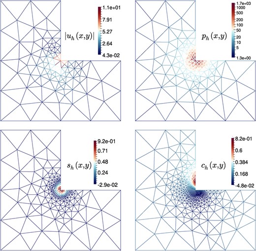
Example 2. Approximate velocity magnitude (after 3 refinement steps), pressure (after 4 refinement steps), concentration |$s$| (after 5 refinement steps) and distribution of |$c$| after 6 steps of adaptive refinement.
Example 3. Experimental errors and convergence rates for the approximate solutions of the transient problem under uniform mesh refinement following the estimator |$\varUpsilon $|, and using the lowest-order scheme with |$k=1$|
| DoF | |$h$| | |$E_{\textbf {u}}$| | rate | |$E_{p}$| | rate | |$E_{s}$| | rate | |$E_{c}$| | rate | |$\texttt {eff}(\varUpsilon )$| |
|---|---|---|---|---|---|---|---|---|---|---|
| 59 | 0.7071 | 0.00228 | – | 0.02080 | – | 0.01811 | – | 0.00711 | – | 0.0859 |
| 195 | 0.3536 | 0.00081 | 1.504 | 0.01191 | 0.843 | 0.00989 | 0.872 | 0.00303 | 1.227 | 0.0970 |
| 707 | 0.1768 | 0.00034 | 1.217 | 0.00621 | 0.940 | 0.00486 | 1.025 | 0.00149 | 1.022 | 0.0973 |
| 2691 | 0.0884 | 0.00015 | 1.119 | 0.00313 | 0.984 | 0.00241 | 1.009 | 0.00074 | 1.008 | 0.0967 |
| 10499 | 0.0442 | 7.70e-05 | 1.053 | 0.00157 | 0.996 | 0.00120 | 1.004 | 0.00031 | 1.003 | 0.0961 |
| 41475 | 0.0221 | 3.78e-05 | 1.025 | 0.00078 | 0.999 | 0.00060 | 1.002 | 0.00018 | 1.001 | 0.0972 |
| 164867 | 0.0110 | 1.87e-05 | 1.012 | 0.00039 | 0.999 | 0.00030 | 1.001 | 9.26e-05 | 1.000 | 0.0966 |
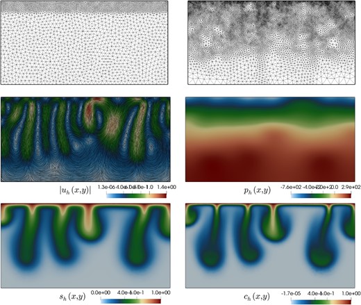
Example 4. Samples of adapted meshes at times |$t=60,1200$| (top panels), and approximate solutions shown at time |$t=1500$| (bottom rows), and computed with a method using |$k=2$|.
6.3 Example 3: robustness of the estimator for the transient problem
Next, we turn to the numerical verification of robustness of the a posteriori error estimator for the fully discrete approximations of the time-dependent coupled problem. We consider now the time interval |$(0,0.01]$| and choose |$\varDelta t =0.002$|. The closed-form solutions on the unit square domain are as follows:
Cumulative errors up to |$t_{\text {final}}$| are computed as
and the resulting error history, after six steps of uniform mesh refinement, is collected in Table 3. Here we have used the lowest-order scheme with |$k=1$|. To be consistent with the development in Section 5, the numerical verification in this set of tests was carried out using a backward Euler time discretization. The a posteriori error estimator (5.1) is computed and the effectivity index is also tabulated, showing that the estimator is robust (and confirming the theoretical reliability bound as well as giving a heuristic indication of its efficiency). Note that in this case, since the mesh refinement is uniform, the auxiliary interpolation of the solutions at the last time step on the current mesh is not necessary. The average number of Newton–Raphson iterations required for convergence was 3.2.
6.4 Example 4: adaptive simulation of exothermic flows
To conclude this section, and to include an illustrative simulation exemplifying that the |$\textbf {H}$|(div)-conforming scheme along with the a posteriori error estimator perform well for an applicative problem, we address the computation of exothermic flows that develop fingering instabilities. The problem configuration is adapted as a simplification of the problem solved in Lenarda et al. (2017) (see also Lee & Kim, 2015; Ruiz-Baier & Lunati, 2016), where the fields |$c,s$| represent solutal concentration and temperature, respectively. The model assumes an additional drag term due to porosity so that the momentum equation is of Navier–Stokes–Brinkman type. The domain is the rectangular region |$\varOmega =(0,L) \times (0,H)$|, and the initial solutal and temperature profiles are imposed as
where |$\zeta _c, \zeta _s$| are random fields uniformly distributed on |$[0,1]$|. The geometric and model constants are |$H=1000$|, |$L=2000$|, |$\varDelta t=20$|, |$t_{\textrm {end}}=1500$|, |$\nu =1 + 0.25\zeta _\nu $|, |$\kappa =1$|, |$1/\text {Sc} = 8$|, |$1/(\tau \text {Sc}) = 2.5$|, |$\rho _{\textrm {m}} = 1$|, |$v_{\textrm {p}} = 0$|, |$\alpha =5$|, |$\beta = -1 $|. The polynomial degree for this example is |$k=2$|.
Boundary conditions are of mixed type for solutal and temperature distribution. Both fields are prescribed to 0 and 1 on the bottom and top of the domain, respectively; while on the vertical walls, we impose zero-flux boundary conditions. The velocity is of slip type on the whole boundary, and therefore a zero-mean condition for the pressure is considered using a real Lagrange multiplier. The solution algorithm, differently from the previous tests, is based on an inner fixed-point iteration between an Oseen and a transport system, rather than an exact Newton–Raphson method. An initial coarse mesh of 5300 elements is constructed, and an adaptive mesh refinement (only one iteration) guided by the estimator (5.1) is applied at the end of each time step, and the algorithm does allow for mesh coarsening. Figure 2 shows snapshots of adapted meshes at different times and also samples of solute concentration, temperature distribution, velocity and pressure at the final time.
Funding
This work has been supported by ANID (Chile) through Fondecyt project 1210610, CMM, project FB210005 of BASAL funds for centers of excellence, CRHIAM, project ANID/FONDAP/15130015, and by Anillo project ANID/ACT210030; by the Sponsored Research and Industrial Consultancy (SRIC), Indian Institute of Technology Roorkee, India through the faculty initiation grant MTD/FIG/100878; by SERB MATRICS grant MTR/2020/000303; by SERB Core research grant CRG/2021/002569; by the Monash Mathematics Research Fund S05802-3951284; by the Ministry of Science and Higher Education of the Russian Federation within the framework of state support for the creation and development of World-Class Research Centers Digital biodesign and personalized healthcare No. 075-15-2022-304; and by the Australian Research Council through the Future Fellowship grant FT220100496 and Discovery Project grant DP22010316.
Data availability
No data was used or generated in this manuscript.
References
Appendix A. Proof of Theorem 2.6
As in the continuous case, using the discrete kernel (2.6) and relying on the inf-sup condition (2.13), we can continue with an equivalent discrete problem without pressure.
