


Abstract
We construct a higher-order adaptive method for strong approximations of exit times of Itô stochastic differential equations (SDEs). The method employs a strong Itô–Taylor scheme for simulating SDE paths, and adaptively decreases the step size in the numerical integration as the solution approaches the boundary of the domain. These techniques complement each other nicely: adaptive timestepping improves the accuracy of the exit time by reducing the magnitude of the overshoot of the numerical solution when it exits the domain, and higher-order schemes improve the approximation of the state of the diffusion process. We present two versions of the higher-order adaptive method. The first one uses the Milstein scheme as the numerical integrator and two step sizes for adaptive timestepping: |$h$| when far away from the boundary and |$h^2$| when close to the boundary. The second method is an extension of the first one using the strong Itô–Taylor scheme of order 1.5 as the numerical integrator and three step sizes for adaptive timestepping. Under some regularity assumptions, we show that for any |$\xi>0$|, the strong error is |${\mathcal{O}}(h^{1-\xi })$| and |${\mathcal{O}}(h^{3/2-\xi })$| for the first and second method, respectively. Provided quite restrictive commutativity conditions hold for the diffusion coefficient, we further show that the expected computational cost for both methods is |${\mathcal{O}}(h^{-1} \log (h^{-1}))$|. This results in a near doubling/trebling of the strong error rate compared to the standard Euler–Maruyama-based approach, while the computational cost rate is kept close to order one. Numerical examples that support the theoretical results are provided, and we discuss the potential for extensions that would further improve the strong convergence rate of the method.
1. Introduction
For a bounded domain |$D \subset{\mathbb{R}}^d$| and a |$d$|-dimensional Itô diffusion |$(X_t)_{t\ge 0}$| with |$X(0) \in D$|, the goal of this work is to construct efficient higher-order adaptive numerical methods for strong approximations of the exit time
where |$T>0$| is given. The dynamics of the diffusion process are governed by the autonomous Itô stochastic differential equation (SDE)
where |$a \colon \mathbb{R}^{d} \to \mathbb{R}^{d}$| and |$b \colon \mathbb{R}^{d} \to \mathbb{R}^{d \times m}$|, |$x_0$| is a deterministic point in |$D$| and |$W$| is an |$m$|-dimensional standard Wiener process on a filtered probability space |$(\varOmega , {\mathcal{F}}, ({\mathcal{F}}_t)_{t \ge 0}, {\mathbb{P}})$|. Further details on the regularity of the domain |$D$| and the coefficients of the SDE are provided in Section 2.
Our method employs a strong Itô–Taylor scheme for simulating SDE paths and carefully decreases the step size in the numerical integration as the solution approaches the boundary of the domain. We present two versions: the order 1 method and the order 1.5 method. The order 1 method uses the Milstein scheme as the numerical integrator and two step sizes for the adaptive timestepping, depending on the proximity of the state to the boundary of |$D$|: a larger timestep when far away and a smaller timestep when close to |$\partial D$|. The order 1.5 method uses the strong Itô–Taylor scheme of order 1.5 as the numerical integrator and, as an extension of the previous method, three different step sizes for the adaptive timestepping.
When adaptive timestepping is properly balanced against the order of the scheme and under sufficient regularity assumptions, then for any |$\xi>0$|, the order 1 method achieves the strong convergence rate |${\mathcal{O}}(h^{1-\xi })$|, cf. Theorem 2.7; and the order 1.5 method achieves the strong convergence rate |${\mathcal{O}}(h^{3/2-\xi })$|, cf. Theorem 2.10. Furthermore, if the diffusion coefficient satisfies the commutativity condition (2.14) for the order 1 method and the conditions (2.14) and (2.18) for the order 1.5 method, then Theorems 2.8 and 2.11 show that both higher-order methods have an expected computational cost of |${\mathcal{O}}(h^{-1} \log (h^{-1}))$|. When applicable, our method nearly preserves the same computational cost as the alternative standard approaches described below, while achieving substantial improvements in the strong convergence rate.
Exit times describe critical times in controlled dynamical systems, and they have applications in pricing of barrier options (Alsmeyer, 1994) and also in American options (Bayer et al., 2020), as the latter may be formulated as a control problem where exit times determine when to execute the option. They also appear in physics, for instance when studying the transition time between pseudo-stable states of molecular systems in the canonical ensemble (Weinan et al., 2021).
The mean exit-time problem may be solved by the Monte Carlo approach of direct simulation of SDE paths or by solving the associated partial differential equation (PDE), the Feynman–Kac equation (Friedman, 1975). In high-dimensional state space, the former approach is more tractable than the latter, due to the curse of dimensionality.
A Monte Carlo method using the Euler–Maruyama scheme with a uniform timestep to simulate SDE paths was shown to produce the weak convergence rate 1/2 for approximating the mean exit time in Gobet (2000). An improved weak order 1 method was achieved by reducing the overshoot error through the careful shifting of the boundary, cf. Broadie et al. (1997); Gobet (2001); Gobet & Menozzi (2004). The weak order 1 method was extended to problems with time-dependent boundaries in Gobet & Menozzi (2010) and Bouchard et al. (2017) showed that in |$L^1(\varOmega )$|-norm, the Euler–Maruyama scheme has an order 1/2 convergence rate. The contributions of this work may be viewed as extensions of this strong convergence study to higher-order Itô–Taylor schemes with adaptive timestepping.
In Jansons & Lythe (2000), a fundamentally different idea for approximating the mean exit time of a one-dimensional Wiener process was developed that reduces the overshoot error using timesteps sampled from an exponential distribution. Numerical simulations show that the method has a weak convergence rate 1. The conditional probability of the stochastic process having exited the domain, given its value at the beginning and at the end of an exponential timestep, is computed, and the process is considered to have exited the domain if this conditional probability is greater than the value of a random variable sampled from the standard uniform distribution. This way, the error committed when computing the empirical probability density function of the exit time is reduced, thereby reducing the overestimation of the mean exit time. The work was later extended to higher-dimensional Wiener process exiting a smooth bounded domain, and then to autonomous scalar SDE in Jansons & Lythe (2005) and Jansons & Lythe (2003), respectively. It remains unclear whether the method can be applied to more general bounded domains and SDE, as well as to multilevel Monte Carlo (MLMC) settings that require strong approximations.
MLMC methods for weak approximations of exit times have been developed in Higham et al. (2013); Giles & Bernal (2018). Using the Euler–Maruyama scheme with boundary shifting and conditional sampling of paths near the boundary, the method (Giles & Bernal, 2018) can reach the mean-square approximation error |${\mathcal{O}}(\epsilon ^2)$| at the near-optimal computational cost |${\mathcal{O}}(\epsilon ^{-2} \log (\epsilon )^2 )$|. Since our methods efficiently approximate the strong exit time and admit a pairwise coupling of simulations on different resolutions, they are also suitable for MLMC. See Section 5 for an outline of the extension to MLMC.
Adaptive methods for SDE with discontinuous drift coefficients have been considered in Neuenkirch et al. (2019); Yaroslavtseva (2022). Therein, the discontinuity regions of the drift coefficient are associated with hypersurfaces. When one is close to such hypersurfaces, a small timestep is used; otherwise, a large timestep is used. This adaptive timestepping approach is similar to ours, as can be seen by viewing the boundary of |$D$| in our problem as a hypersurface, but the problem formulations differ, and our method is more general in the sense that it admits a sequence of timestep sizes and also higher-order numerical integrators. For numerical testing of strong convergence rates, we have employed the idea of pairwise coupling of non-nested adaptive simulations of SDE developed in Giles et al. (2016), which is an approach that also could be useful for combining our method with MLMC in the future. See also Merle & Prohl (2023) for a recent contribution on a posteriori adaptive methods for weak approximations of exit times and states of SDE, and Hoel et al. (2012); Katsiolides et al. (2018); Fang & Giles (2020) for other partly state-dependent adaptive MLMC methods for weak approximations of SDE in finite- and infinite-time settings.
The Walk-On-Spheres (WoS) method (Muller, 1956; Deaconu et al., 2017) is an alternative approach for weak approximations of exit points of bounded diffusions that relies on simulations of SDE paths whose increments typically are bounded in the state-space rather than in the timestep. WoS requires closed-form expressions or a tractable approximation of exit time distributions of spheres, or other suitable surfaces like cubes or ellipsoids, so that the exit time of the process can be generated from walking/hopping on such surfaces. For more general SDE, extensions of WoS that rely on such principles have been developed, including error- and complexity analysis, for weak approximations of exit points and for reflected diffusions on bounded domains by Milstein et al. (Milstein, 1996, 1997; Milstein & Tretyakov, 2004). See also Leimkuhler et al. (2023) for extensions of Milstein’s WoS method to settings with more complicated boundary conditions and over infinite time-windows. Improvements to the practical implementation of Milstein’s WoS method for bounded diffusions and efficient estimation of a point’s distance to the boundary are further explored in Bernal (2019).
Unlike our approach, the efficiency of Milstein’s WoS method is not limited by commutativity conditions on the diffusion coefficient. But we believe our method is more suitable for extension to MLMC and thus to exploit the potential efficiency gains that offer for weak approximations, as it is easy to construct the kind of pairwise coupled realizations on neighboring resolution levels needed in MLMC with our method.
The rest of this paper is organized as follows: Section 2 presents two versions of the higher-order adaptive method and states the main theoretical results on convergence and computational cost. Section 3 contains proofs of the theoretical results. Section 4 presents a collection of numerical examples supporting our theoretical results. Lastly, we summarize our findings and discuss interesting open questions in Section 5.
2. Notation and the adaptive numerical methods
In this section, we first introduce the necessary notation and assumptions on the SDE coefficients and the domain |$D$|, and relate the exit-time problem to the Feynman–Kac PDE. Thereafter, the higher-order adaptive methods of order 1 and 1.5 are respectively described in Sections 2.4 and 2.5, with convergence and computational cost results.
2.1 Notation and assumptions
For any |$x,y \in{\mathbb{R}}^d$|, the Euclidean distance is denoted by |$d(x,y):= |x-y|$|, and for any nonempty sets |$A,B \subset{\mathbb{R}}^d$|, we define
A domain in |${\mathbb{R}}^d$| is defined as an open, nonempty and connected subset of that space. The following assumptions on the domain of the diffusion process will be needed to relate the exit-time problem to a sufficiently smooth solution of a Feynman–Kac PDE.
The domain |$D \subset{\mathbb{R}}^d$| is bounded and the boundary |$\partial D$| is |$C^{4}$| continuous.
Let |$n_D:\partial D \to{\mathbb{R}}^d$| denote the outward-pointing unit normal and for any |$r>0$|, let
Due to the regularity of the boundary, it holds that |$n_D \in C^{3}(\partial D,{\mathbb{R}}^d)$| and |$D$| satisfies the uniform ball property: there exists an |$R>0$| such that for every |$x \in{\mathbb{R}}^n$| such that |$d(x,\partial D)< R$|, there is a unique nearest point |$y$| on the boundary |$\partial D$|, and it holds that |$x = y \pm d(x,y) n_D(y)$|, where the sign |$\pm $| depends on whether |$x$| belongs to the exterior or interior of |$D$|. (That is, for every |$x$| sufficiently close to the boundary, there is a unique point on |$\partial D$| satisfying that |$y = \arg \min _{z \in \partial D} d(x,z)$|.) We refer to Gilbarg & Trudinger (2001, Chapter 14.6) for further details on the regularity of |$\partial D$| and its unit normal |$n_D$|, and to Dalphin (2014, Theorem 1.9) for the uniform ball property. For any domain |$D$| satisfying the uniform ball property, let |$\textrm{reach}(D)> 0$| denote the supremum of all |$R>0$| such that the property is satisfied. The uniform ball property is equivalent to satisfying both the uniform exterior sphere and the interior sphere conditions.
For any |$r\in (0, \textrm{reach}(D))$|, the boundary of |$D_r$| can be expressed by
and, since the mapping
is a |$C^3$|-diffeomorphism and |$\partial D$| is |$C^4$|, it follows that |$\partial D_r$| is at least |$C^3$|. This implies that |$D_r$| also satisfies the uniform ball property, and since any point |$z \in \partial D_r$| can be expressed as |$z= y + r n_D(y)$| for a unique |$y \in \partial D$| and indeed |$n_D(y) = n_{D_r}(z)$|, it follows that the reach of |$D_r$| is bounded from below by |$\textrm{reach}(D)-r$|, which we state for later reference:
A similar construction applies to the boundary of the subdomain |$D_{-r}:= \{x \in D \mid d(x, \partial D)>r \}$|, where one can show that |$\partial D_{-r}$| is at least |$C^3$| for all |$r \in (0,\textrm{reach}(D))$|.
For any integer |$k\ge 1$|, let |$C^{k}_b({\mathbb{R}}^d)$| denote the set of scalar-valued functions with continuous and uniformly bounded partial derivatives up to and including order |$k$|. We make the following assumptions on the coefficients of the SDE (1.2).
- (B.1) For the SDE coefficientsit holds that |$a_i, b_{ij} \in C_b^{3}({\mathbb{R}}^d)$| for all |$i \in \{1,\ldots ,d\}$| and |$j \in \{1,\ldots , m\}$|.$$ \begin{align*} & a(x) = \begin{bmatrix} a_1(x) \\ \vdots \\ a_d(x) \end{bmatrix} \qquad \textrm{and} \qquad b(x) = \begin{bmatrix} b_{11}(x) & \cdots & b_{1m}(x)\\ \vdots & & \vdots \\ b_{d1}(x)& \cdots & b_{dm}(x) \end{bmatrix} \end{align*} $$
- (B.2) (Uniform ellipticity) For some |$\bar R_D \in (0,\textrm{reach}(D)/2)$|, there exists a constant |$\hat c_b>0$| such that$$ \begin{align*} & \hat c_{b} \left| {\xi} \right|^{2} \le \xi^{\top} (b(x) b^{\top}(x)) \xi \qquad \forall (x, \xi) \in D_{\bar R_D} \times{\mathbb{R}}^d. \end{align*} $$
- (B.3) There exists a constant |$\widehat C_{b}> 0$| such that$$ \begin{align*} & \xi^{\top} \!\big( {b(x) b^{\top}(x)} \big) \xi \le \widehat C_{b} \left| {\xi} \right|^{2}, \qquad \forall (x,\xi) \in \mathbb{R}^{d}\times \mathbb{R}^{d}. \end{align*} $$
Assumption B.1 ensures well-posedness of strong exact and numerical solutions of the SDE (1.2) and is sufficient to obtain the sought for regularity for the solution of the Feynman–Kac PDE in Propositions 2.3 and 2.4.
B.2 ensures that the diffusion process will, loosely speaking, eventually exit the domain, and it is used to obtain well-posedness of the related Feynman–Kac PDE in Propositions 2.3 and 2.4. B.3 is introduced to bound the magnitude of the overshoot of numerical paths of the diffusion process when they exit |$D$|.
This is because any |$C^{3}$|-redefinition of all coefficients on |$\overline D^C$| such that |$a_i, b_{ij} \in C^{3}_b({\mathbb{R}}^d)$| will not change the exit time of the resulting diffusion process.
2.2 Mean exit times and Feynman–Kac
Recalling that the exit time was defined by |$\tau = \inf \{t \ge 0 \mid X(t) \notin D \} \wedge T$|, we extend this notation to the time-adjusted exit time of a path going through the point |$(t,x)\in [0,T] \times{\mathbb{R}}^d$|:
Since |$X(0) = x_0$| for the diffusion process (1.2), we note that |$\tau = \tau ^{0,x_0}$|. Under sufficient regularity, the mean (time-adjusted) exit time
solves the following parabolic PDE:
To bound the overshoot of the exit time of numerical solutions, it is useful to study time-adjusted exit times on domains |$D_r$| for any |$r \in [0,\bar R_D]$|, where |$\bar R_D$| is defined in Assumption B.2. For any |$(x,t) \in [0,T] \times D_r$|, let
Similarly as for the exit time for the domain |$D$|, we introduce the shorthand |$\tau _r:= \tau _r^{0,x_0}$|. The mean exit time for the enlarged domain is defined by
The function |$u_r(t,x)$| is also the unique solution of a Feynman–Kac equation:
Existence, uniqueness and regularity of the solution to the elliptic PDE (2.7) can be shown to hold under weaker regularity assumptions on coefficients, domain and boundary values (Gilbarg & Hörmander, 1980, Theorems 6.1, 6.2, 6.3).
2.3 Higher-order adaptive numerical methods
Let |$\gamma \in \{1,3/2\}$| denote the order of the strong Itô–Taylor method used in the numerical integration of the SDE (1.2), cf. Kloeden & Platen (1992, Chapter 10). In abstract form, our numerical method simulates the SDE (1.2) by the scheme
where |$\overline{X}(0) = x_0$| and |$\varPsi _\gamma : {\mathbb{R}}^d \times [0,\infty ) \times \varOmega \to{\mathbb{R}}^d$| denotes the higher-order Itô–Taylor scheme. The timestep |$\varDelta t_n = \varDelta t(\overline{X}(t_n))$| is adaptively chosen as a function of the current state |$\overline{X}(t_n)$| so that the step size is small when |$\overline{X}(t_n)$| is near the boundary |$\partial D$|, and larger otherwise. Both the integrator |$\varPsi _\gamma $| and the adaptive timestepping depend on the order of |$\gamma $|, see Sections 2.4 and 2.5 below for further details. The purpose of the adaptive strategy is to reduce the magnitude of the overshoot when the numerical solution exits |$D$|, and the stochastic mesh
is a sequence of stopping times with |$t_{n+1}$| being |${\mathcal{F}}_{t_n}$|-measurable for all |$n=0,1,\ldots $|. The exit time of the numerical method is defined as the first time |$\overline{X}(t_n)$| exits the domain |$D$|:
and we will use the following notation for the time mesh of the numerical solution up to or just beyond |$T$|:
For later analysis, the domain of definition for the numerical solution is extended to a piecewise constant solution over continuous time by
Sections 2.4 and 2.5 below present the details for the order 1 and order 1.5 adaptive methods, respectively.
2.4 Order 1 method
The |$i$|th component of the strong Itô–Taylor scheme (2.8) of order |$\gamma =1$| is given by
for |$i \in \{1,\ldots , d\}$|, where we have introduced the shorthand |$\varDelta W^j_n = W^j(t_{n+1}) - W^j(t_n)$| for the |$n$|th increment of the |$j$|th component of the Wiener process, the operator
and the iterated Itô integral
of the components |$(j_1,j_2) \in \{1,\ldots ,m\} \times \{1,\ldots ,m\}$|.
The size of |$\varDelta t_n$| is determined adaptively by the state of the numerical solution. A small step size is employed when |$\overline{X}(t_n)$| is close to the boundary |$\partial D$|, to reduce the magnitude of the overshoot of an exit of the domain and the likelihood of the numerical solution not capturing a true exit of the domain; and a larger step size is employed when |$\overline{X}(t_n)$| is farther away from the boundary. For any |$b>a\ge 0$|, we introduce the following notation to describe the distance from the boundary:
Introducing the step size parameter |$h \in (0,1)$| and the threshold parameter
the ‘critical region’ of points near the boundary is given by
and the adaptive timestepping by
This means that a large timestep is used when the |$\overline{X}(t_n)$| is in the noncritical region |$D\setminus V_{\partial D}(0, \delta )$| and a small step size |$h^{2}$| in the critical region near the boundary. (The step size used in |$D^C$|, whether |$h$| or |$h^2$|, is not of any practical importance for the output of the numerical method. But in our theoretical analysis we need to compute the numerical solution up to time |$T$|, and in case |$\nu < T$|, the step size for |$\overline{X}(t_n) \in D^C$| needs to be described to compute the solution for times in |$(\nu ,T]$|.) The value of the parameter |$\delta $| is chosen as a compromise between accuracy and computational cost: it should be sufficiently large so that the strong-error convergence rate in |$h$| is kept at almost order 1, cf. Theorem 2.7, but it should also be as small as possible to keep the computational cost of the method low. From the proofs of Lemma 3.3 and Theorem 2.8, it follows that the formula (2.16) is a suitable compromise for |$\delta $|.
We are now ready to present the main results on the strong convergence rate and computational cost of the order 1 method.
To study the complexity of the method, we first define the computational cost of a numerical solution as the number timesteps used to compute the exit time:
Observe that |$\textrm{Cost}\!\left ({\nu }\right )$| is a random variable since the exit time |$\nu $| is different for each realization of the numerical solution. We further make the assumption that every evaluation of the distance of the numerical solution |$\overline{X}(t)$| to the boundary of the domain |$\partial D$|, required for adaptive refinement of timestep size, costs |${\mathcal{O}}(1)$|. This is a limiting assumption, as it can be challenging to compute the distance to the boundary in more complicated domains. On that note, the distance function |$d(x,\partial D)$| is the solution of an Eikonal equation (Bernal, 2019), and it can be approximated numerically using Sethian’s fast marching method (Sethian, 1996).
The proof of Theorem 2.8 uses an occupation-time estimate of the time the numerical solution spends in the critical region before exiting. Near-boundary occupation-time estimates have appeared frequently in the literature, as they often are useful tools for bounding approximation errors and complexity. For an SDE with low-regularity drift functions, the occupation-time on discontinuity sets is used to bound the computational cost of the adaptive method in Neuenkirch et al. (2019); Yaroslavtseva (2022). When |$d=1$|, the approach (Yaroslavtseva, 2022) carries over to our order 1 method. For |$d>1$|, occupation-time estimates using local time manipulations have been derived for the Euler–Maruyama method for diffusion processes (Neuenkirch et al., 2019, Lemma 3.3) and hypoelliptic diffusion processes (Gobet & Menozzi, 2004, Lemma 19).
2.5 The order 1.5 method
The general strong Itô–Taylor scheme of order |$\gamma =1.5$| is a complicated expression that can be found in Kloeden & Platen (1992, equation (10.4.6)). When the so-called second commutativity condition holds:
where the differential operator |${\mathcal{L}}^j$| is defined in (2.12), then the scheme simplifies to a practically useful form where the computational cost of one iteration of |$\varPsi _{1.5}$| is |${\mathcal{O}}(1)$|, cf. Kloeden & Platen (1992, equation (10.4.15)). And in the special case of (2.18), when the diffusion coefficient is a diagonal matrix, the |$i$|th component of the scheme takes the form
where we have introduced the differential operator
and
For computer implementations, let us add that the tuple of correlated random variables |$(\varDelta W^i_n, \varDelta Z_n^i)$| can be generated by
where |$U_1$| and |$U_2$| are independent |$N(0,1)$|-distributed random variables.
The step size |$\varDelta t_n$| for the order 1.5 method is determined adaptively by the state of the numerical solution, but with one more resolution than for the order 1 method: a tiny step size is employed when |$\overline{X}(t_n)$| is very close to the boundary |$\partial D$|, a small step size is employed when |$\overline{X}(t_n)$| is slightly farther away from the boundary, and the largest step size is employed when it is far away from the boundary. To describe this mathematically, we first introduce the step size parameter |$h \in (0,1)$|, the threshold parameters
and the critical regions
and
The timestepping is then given by
This means that the step size |$h$| is used when |$\overline{X}(t_n)$| is in the noncritical region |$D\setminus V_{\partial D}(0, \delta _1)$|, the small step size |$h^2$| is used when |$\overline{X}(t_n)$| is in the critical region farthest from the boundary and the tiny step size |$h^3$| is used when |$\overline{X}(t_n)$| is in the critical region nearest the boundary. (The step size used in |$D^C$|, whether |$h$|, |$h^2$| or |$h^3$| is not of any practical importance, but is needed in the theoretical analysis to extend the numerical solution up to time |$T$| when |$\nu < T$|, similarly as for the order 1 method.) The values of the threshold parameters |$(\delta _1, \delta _2)$| are chosen as a compromise between accuracy and computational cost: The critical regions should be sufficiently large so that the strong-error convergence rate in |$h$| is kept at almost order 1.5, cf. Theorem 2.10, but they should also be kept as small as possible to keep the computational cost of the method low. It follows from the proofs of Lemma 3.4 and Theorem 2.11 that (2.20) is a suitable compromise.
We are now ready to present the main results on the strong convergence rate and computational cost of the order 1.5 method.
3. Theory and proofs
This section proves theoretical properties of the adaptive timestepping methods of order 1 and 1.5. We first describe how critical regions combined with adaptive timestepping can bound the overshoot of the diffusion process with high probability, and thereafter use this property to prove the strong convergence of the method given by Theorems 2.7 and 2.10. Lastly, we prove upper bounds for the expected computational cost of the methods.
Let us first state a few theoretical results that will be needed in later proofs.
3.1 Order 1 method
This section proves theoretical results for the order 1 method.
For the Itô process (1.2) and |$t>s\ge 0$|, let
One may view |$M(s,t)$| as the maximum stride the process |$X$| takes over the interval |$[s,t]$|. The lemma below shows that the threshold parameter |$\delta $| is chosen sufficiently large to ensure that the maximum stride |$X$| takes over every interval in the mesh |${\mathcal{T}}^{\varDelta t}$| is with very high probability bounded by |$\delta $|. This estimate will help us bound the probability that the numerical solution exits the domain |$D$| from the noncritical region in the proof of Theorem 2.7 (i.e., to bound the probability of exiting |$D$| when using a large timestep).
We next prove the computational cost result for the order 1 method.
3.2 Order 1.5 method
This section proves theoretical results for the order 1.5 method.
The lemma below shows that the threshold parameters |$\delta _1$| and |$\delta _2$| are chosen sufficiently large to ensure that the maximum stride |$X$| takes over every interval in the mesh |${\mathcal{T}}^{\varDelta t}$| is with high likelihood bounded by either |$\delta _1$| or |$\delta _2$|, depending on the length of the interval. The estimate will help us bound the probability that the numerical solution exits the domain |$D$| from anywhere, but the critical region nearest the boundary of |$D$| in the proof of Theorem 2.10 (i.e., bound the probability of exiting |$D$| using a larger timestep than |$h^3$|).
Up next, we prove the computational cost result for the order 1.5 method.
4. Numerical experiments
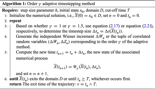
We run several simulations to numerically verify the theoretical rates for strong convergence and computational cost for the order 1 and 1.5 methods. Algorithm 1 describes the implementation of the two methods for computing the exit time of one SDE path. In all the problems below, we consider exit times (1.1) with cut-off time |$T=10$|.
4.1 Geometric Brownian Motion
For the one-dimensional geometric Brownian motion
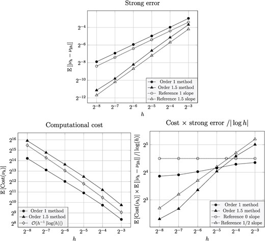
we consider the exit time from the interval |$D = (1, 7)$|. The reference solution to the mean exit time was computed by numerically solving the Feynman–Kac PDE, cf. Proposition 2.3, using the Crank–Nicolson method for time discretization and continuous, piecewise linear finite elements for spatial discretization. For this purpose, we use the Gridap.jl library (Badia & Verdugo, 2020; Verdugo & Badia, 2022) in the Julia programming language. The pseudo-reference solution for the mean exit time of the process starting at |$\overline{X}(0) = 4$| is |${\mathbb{E}}_{} \left [ {\tau } \right ] = 7.153211$|, rounded to 7 significant digits. We let |$\nu _h$| denote the exit time of the numerical solution |$\overline{X}$| from the domain |$D$| using the |$h>0$|. Monte Carlo estimates with |$M= 10^7$| samples are used to estimate the strong error
and the computational cost
Realizations on neighboring resolutions |$\nu _{h}^i$| and |$\nu _{2h}^i$| are pairwise coupled using the technique for non-nested meshes introduced in Giles et al. (2016) together with the procedure (Hoel & Krumscheid, 2019, Example 1.1) for coupling all driving noise in the order 1.5 method. This reduces the variance of the samples |$\nu _h^i - \nu _{2h}^i$| in the Monte Carlo estimators, leading to a more efficient Monte Carlo estimator.
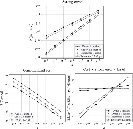
Numerical tests for the exit-time problem in Section 4.1: Strong error (top), computational cost (bottom left) and cost |$\times $| strong error (bottom right).
Figure 1 shows that the strong convergence rate obtained from the numerical simulations agrees with the theory for the order 1 and order 1.5 methods and the weak convergence rate coincides with the strong rate. In alignment with theory, we further observe that the expected computational cost for both adaptive methods are |${\mathcal{O}}(h^{-1} \left | {\log (h)} \right |)$| and that
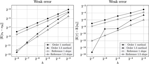
Lastly, we approximate the weak error |$|{\mathbb{E}}_{} \left [ {\tau - \nu _h} \right ]|$| numerically by Monte Carlo in two different ways. First, using pairwise coupled realizations,
with |$M=4 \times 10^7$| samples. And second, using the aforementioned pseudo-reference solution of |${\mathbb{E}}_{} \left [ {\tau } \right ]$| computed with the finite element method, we sample
using |$M=4\times 10^7$| number of samples. Since the variance of |$\nu _h - \nu _{2h}$| is much smaller than that of |${\mathbb{E}}_{} \left [ {\tau } \right ] -\nu _h$| when |$h$| is sufficiently small, the last approach to estimating the weak error is more sensitive to statistical error and thus less tractable than the first one. We have nonetheless included the last approach to also verify numerically that our estimator |$\nu _h$| asymptotically is unbiased |$\big($|since |$\lim _{h \downarrow 0} {\mathbb{E}}_{} \left [ {\nu _h} \right ] = {\mathbb{E}}_{} \left [ {\nu } \right ]$| does not directly follow from |$\lim _{h \downarrow 0} |{\mathbb{E}}_{} \left [ {\nu _h -\nu _{2h}} \right ]\!|=0\big)$|. Figure 2 shows the weak convergence rate |${\mathcal{O}}(h^\gamma )$| for the respective adaptive methods.
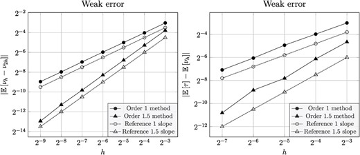
Numerical tests of the weak error for the exit-time problem in Section 4.1.

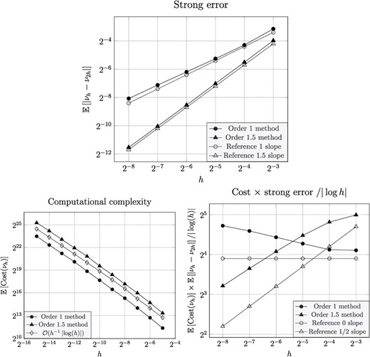
Numerical tests for the exit-time problem in Section 4.2: strong error (top), computational cost (bottom left) and cost |$\times $| strong error (bottom right).
4.2 Linear drift, cosine diffusion coefficient—1D
For the SDE
we study the exit time from the interval |$D = (1, 7)$|. The pseudo-reference solution to the mean exit-time problem was computed by solving the Feynman–Kac PDE using the same numerical method as in the preceding example, yielding |${\mathbb{E}}_{} \left [ {\tau } \right ] = 5.504741$|, rounded to 7 significant digits. Weak and strong errors and the computational cost of the adaptive methods are estimated using Monte Carlo with the same number of samples as in the preceding example.
Figure 3 shows numerical estimates of the strong error and the computational cost. Taking into account that the strong-error estimate is sensitive to statistical errors for small values of |$h$|, the observed rates for the strong error and computational cost are consistent with theory.
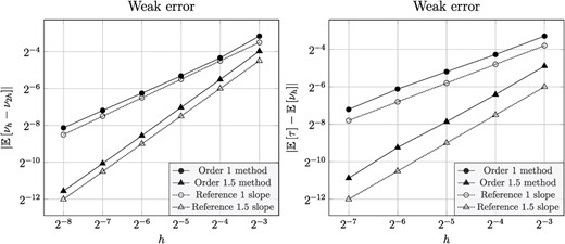
Figure 4 shows that the weak convergence rate is |${\mathcal{O}}(h^\gamma )$| for the respective adaptive methods.
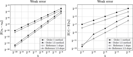
Numerical tests of the weak error for the exit-time problem in Section 4.2.
We next consider two higher-dimensional exit-time problems.
4.3 Linear drift, linear diffusion—2D
We consider the SDE
with initial condition |$ X(0) = (3, 3)^{\top }$|, and we are interested in computing the exit time from the disk
The pseudo-reference solution to the mean exit-time problem is computed by numerically solving the Feynman–Kac PDE, yielding |${\mathbb{E}}_{} \left [ {\tau } \right ] = 6.7737$|, rounded to 5 significant digits. Weak and strong errors, and the computational cost of the adaptive methods are estimated using Monte Carlo with the same number of samples as in the previous examples.
Figure 5 shows numerical estimates of the strong error and computational cost, and Fig. 6 shows the estimates for the weak error. The observed rates for the strong error and the computational cost are once again consistent with theory. For the 1.5 order method, the weak error tests further indicate that the weak convergence rate may be slightly higher than 1.5, for this problem.
Numerical tests for the exit-time problem in Section 4.3: Strong error (top), computational cost (bottom left) and cost |$\times $| strong error (bottom right).
Numerical tests of the weak error for the exit-time problem in Section 4.3.
4.4 Linear drift, cosine diffusion—2D
We consider the following two-dimensional SDE with linear drift and nonlinear, diagonal diffusion coefficient:
and with initial condition |$X(0) = (3, 3)^{\top }$|. Note that the components of the SDE are coupled through the drift term, similarly as for the SDE in Section 4.3. We compute the exit time of the SDE from the disk domain given by equation (4.6). The reference solution to the mean exit-time problem is computed by numerically solving the Feynman–Kac PDE, yielding |${\mathbb{E}}_{} \left [ {\tau } \right ] = 5.0853$|, rounded to 5 significant digits.
Monte Carlo estimates of strong and weak errors are estimated using the same number of samples and over the same ranges of |$h$|-values as in the previous example. But since the asymptotic regime of the computational cost seems to appear later—for smaller |$h$|-values—for this problem than the previous ones, we have estimated it over a range of smaller |$h$|-values, |$h \in [2^{-5}, 2^{-15}]$|, using |$M=10^3$| samples (this seems to suffice as the cost estimate does not appear sensitive to the sample size).
Figure 7 shows numerical estimates of the strong error and computational cost, and Fig. 8 shows the estimates for the weak error. The observed rate for the strong error is consistent with theory. We note that the asymptotic regime for the computational cost is not reached before |$h<2^{-10}$| for neither of the methods, but that it looks proportional to |$h^{-1} |\!\log (h)|$| near the smallest |$h$|-values. As for the previous example, we also include a Monte Carlo estimate of computational cost times the strong error, cf. (4.3). This result is consistent with theory for the order |$1.5$| method, but inconclusive for the order |$1$| method. We believe this is because, as mentioned above, the |${\mathbb{E}}_{} \left [ {\textrm{Cost}\!\left (\nu _h\right )} \right ]$| function has not reached its asymptotic regime in the window of |$h$|-values that we can afford to study numerically, and that also the order |$1$| method will produce test results that are consistent with theory for sufficiently small |$h$|-values.
Numerical tests for the exit-time problem in Section 4.4: Strong error (top), computational cost (bottom left) and cost |$\times $| strong error (bottom right).
Numerical tests of the weak error for the exit-time problem in Section 4.4.
5. Conclusion
In this paper, we developed a tractable higher-order adaptive timestepping method for the strong approximation of Itô-diffusion exit times. The fundamental idea is to use smaller step sizes as the numerical solution gets closer to the boundary of the domain, and to use higher-order integration schemes for better approximation of the state of the Itô diffusion. This reduces both the magnitude of the overshoot when the numerical solution exits the domain and the probability of the numerical solution missing an exit of the domain by the exact process.
We theoretically proved that the Milstein scheme combined with adaptive timestepping with two different step sizes lead to a strong convergence rate of |${\mathcal{O}}(h^{1-})$|, and that the strong order 1.5 Itô–Taylor scheme combined with adaptive timestepping with three different step sizes lead to a strong convergence rates of |${\mathcal{O}}(h^{3/2-})$|. We also showed that if the diffusion-coefficient commutativity conditions (2.14) and (2.18) hold, then the expected computational cost for both methods is bounded by |${\mathcal{O}}(h^{-1} \left | {\log (h)} \right |)$|. Many diffusion coefficients with off-diagonal terms do not satisfy these conductivity conditions, and, although efficient when applicable, this does unfortunately limit the scope of our method considerably more than for example Milstein’s WoS methods.
There are several interesting ways to extend the current work. One direction would be to consider strong Itô–Taylor schemes of order |$\gamma> 3/2$| combined with adaptive timestepping that employs more than two critical regions, i.e., for some |$h \in (0, 1)$|, we consider timestep sizes finer than |$h^{3}$| when the numerical solution is very close to the boundary |$\partial D$|. This way, the strong convergence rate can be further improved while maintaining a computational complexity that is tractable. Another direction could be to extend the adaptive method to exit-time problems on more general domains, such as half-spaces or domains that may evolve in time, cf. Gobet (2001); Gobet & Menozzi (2010).
Although our adaptive method has been devised for improving the strong convergence rate of exit times of Itô-diffusions, the results easily extend to weak approximations of quantities of interest (QoI) that depend on the exit time and the state of the process:
where we assume that |$f, g$| are functions that are sufficiently smooth.
For weak approximations, the combination of MLMC and adaptive timestepping can lead to substantial efficiency gains over standard Monte Carlo methods, cf. Hoel et al. (2012, 2014); Giles et al. (2016); Katsiolides et al. (2018); Kelly & Lord (2018); Fang & Giles (2020). A key component in the MLMC method is to achieve strong pairwise coupling of fine- and coarse resolution trajectories of the stochastic process. A smart way to couple solutions of the Euler–Maruyama method on non-nested adaptive meshes has been developed in Giles et al. (2016), and it would be interesting to study how extensible that approach is to our higher-order methods, using for instance the coupling procedure in Hoel & Krumscheid (2019, Example 1.1).
Finally, in Giles & Bernal (2018), a new MLMC methodology to compute the mean exit time or a QoI that depends on the exit time of a stochastic process was developed. The new MLMC method reduces the multilevel variance by computing the approximate conditional expectation once the coarse or fine trajectory has exited the domain. Combining our ideas on higher-order adaptive timestepping with the conditional MLMC method has the potential to reduce the computational cost of exit time simulations even further. This makes an interesting problem for future research.
Acknowledgements
We would like to thank Mike Giles for suggestions on improving the manuscript, particularly for the very nice idea to use the absorbing-boundary Fokker–Planck equation in the proof of the computational cost of the adaptive methods. This improved our computational cost result considerably! We also thank Snorre Harald Christensen, Kenneth Karlsen, Peter H.C. Pang and Nils Henrik Risebro for helpful discussions on parabolic and elliptic PDE, and the anonymous referees for very helpful remarks.
Funding
Mathematics Programme of the Trond Mohn Foundation.
References
Appendix. A. Theoretical results
Appendix. B. Computational cost for the order 1 method—1D Wiener process
In this section, we use a simple approach to derive an upper bound for the computational cost of implementing the order 1 adaptive method for a one-dimensional Wiener process |$W(t)$| exiting the interval |$(a, b)$|. This is possible thanks to the availability of the joint density of |$W(t)$| and its running maximum/minimum.
Let |$\overline{W}(t)$| denote the continuous-time extension of the discretely sampled Wiener process. For |$t> s \geq 0$|, let |$M_{W}(s, t)$| and |$m_{W}(s, t)$| denote the running maximum and the running minimum of the one-dimensional Wiener process |$W(t)$|, respectively, over the interval |$[s, t]$|, i.e.,
Let the shorthands |$M_{W}(t)$| and |$m_{W}(t)$| represent the running maximum and the running minimum of the Wiener process over the interval |$[0, t]$|, respectively. Recall that the running maximum and the negative of the running minimum of the Wiener process have the same distribution, cf. Klebaner (2012, Section 3.6).
The threshold parameter |$\delta (h)$|, for all |$h \in (0, 1)$|, is defined as
We construct the set |$A$| to bound the strides of the running maximum and the running minimum of the Wiener process
For all |$h < e^{-1}$| and |$\delta (h)$| given by (B.1), it can be shown similarly as in the proof of Lemma 3.3 that
