


Abstract
We propose some new mixed finite element methods for the time-dependent stochastic Stokes equations with multiplicative noise, which use the Helmholtz decomposition of the driving multiplicative noise. It is known (Langa, J. A., Real, J. & Simon, J. (2003) Existence and regularity of the pressure for the stochastic Navier--Stokes equations. Appl. Math. Optim., 48, 195--210) that the pressure solution has low regularity, which manifests in suboptimal convergence rates for well-known inf-sup stable mixed finite element methods in numerical simulations; see Feng X., & Qiu, H. (Analysis of fully discrete mixed finite element methods for time-dependent stochastic Stokes equations with multiplicative noise. arXiv:1905.03289v2 [math.NA]). We show that eliminating this gradient part from the noise in the numerical scheme leads to optimally convergent mixed finite element methods and that this conceptual idea may be used to retool numerical methods that are well known in the deterministic setting, including pressure stabilization methods, so that their optimal convergence properties can still be maintained in the stochastic setting. Computational experiments are also provided to validate the theoretical results and to illustrate the conceptual usefulness of the proposed numerical approach.
1. Introduction
When |$ \textbf {B} \equiv \textbf {0}$|, (1.1) is the well-known (deterministic) Stokes system; one motivation for studying (1.1a)–(1.1b) with ‘random force’ |$\mathbf {f}+ \textbf {B}( \textbf {u})\frac {\textrm{d}W}{\textrm{d}t}$| is to develop mathematical models of this type for turbulent fluids (Bensoussan, 1995; Hairer & Mattingly, 2006). In addition to their importance in applied sciences and engineering, the Stokes equations are a well-known partial differential equation (PDE) model with saddle point structure, which requires special numerical discretizations to construct optimally convergent methods. It should be noted that although the involved deterministic Stokes operator is linear, system (1.1a)–(1.1b) is nonlinear due to the nonlinear function |$ \textbf {B}$|.
inf-sup stable mixed finite element methods require |$H^1$|-regularity of the pressure in order to optimally bound the best-approximation error for the pressure, which leads to optimal-order convergence; cf. Brezzi & Fortin (1991), Girault & Raviart (1986), Heywood & Rannacher (1982);
stabilization methods require |$H^1$|-regularity of the pressure for convergence; cf. Hughes et al. (1986), Prohl (1997).
The above consideration crucially affects the error analysis of a space-time discretization of (1.1a)–(1.1b):
Exactly divergence-free methods require restricted settings of data, including the dimension, topology and regularity of the spatial domain |$D$|. However, an optimal-order error estimate can be proved for the velocity approximation; see Carelli & Prohl (2012), which uses the fact that no pressure is involved in the analysis.
The error estimate for the velocity approximation of inf-sup stable mixed finite element methods in Feng & Qiu (2019) was obtained based on a stability bound of type (1.5) to bound the related best-approximation error for the pressure that appears in (an auxiliary temporal discretization of) (1.1), thus leading to a sub-optimal error estimate for the velocity of order |${\mathcal O}(k^{\frac 12} + h {k}^{-\frac 12})$|. The computational studies in Feng & Qiu (2019) suggest that this error bound is sharp.
The remainder of this paper is organized as follows. In Section 2 we give exact assumptions on the data in (1.1) and recall the definition and known properties of the (strong) variational solution for problem (1.1). In Sections 3 and 4 we analyze the Helmholtz decomposition enhanced Euler–Maruyama time-stepping scheme (1.6)–(1.7) and its mixed finite element approximations and establish optimal convergence for both. Section 5 establishes optimal convergence for the stabilized scheme (1.9) and its equal-order finite element approximations. Two-dimensional numerical experiments and computational studies are given in Section 6 to validate the theoretical error bounds and to computationally evidence that a proper selection of the pressure for the construction of optimally convergent mixed methods is indeed necessary.
2. Preliminaries
2.1 Notation
Standard function and space notation will be adopted in this paper. For example, |$H^\ell _\textrm{per}(D, {\mathbb R}^d)\, (\ell \geq 0)$| denotes the subspace of the Sobolev space |$H^\ell (D, {\mathbb R}^d)$| consisting of |${\mathbb R}^d$|-valued periodic functions with period |$L$| in each spatial coordinate direction and |$(\cdot ,\cdot ):=(\cdot ,\cdot )_D$| denotes the standard |$L^2$|-inner product, with induced norm |$\Vert \!\cdot\! \Vert $|. Let |$(\varOmega ,{\mathcal {F}}, \{{\mathcal {F}}_t\},{\mathbb {P}})$| be a filtered probability space with the probability measure |${\mathbb {P}}$|, the |$\sigma $|-algebra |${\mathcal {F}}$| and the continuous filtration |$\{{\mathcal {F}}_t\} \subset {\mathcal {F}}$|. For a random variable |$v$| defined on |$(\varOmega ,{\mathcal {F}}, \{{\mathcal {F}}_t\},{\mathbb {P}})$|, let |${\mathbb E}[v]$| denote the expected value of |$v$|. For a vector space |$X$| with norm |$\|\cdot \|_{X}$|, and |$1 \leq p < \infty $|, we define the Bochner space |$\bigl (L^p(\varOmega ,X); \|v\|_{L^p(\varOmega ,X)} \bigr )$|, where |$\|v\|_{L^p(\varOmega ,X)}:=\bigl ({\mathbb E} [ \Vert v \Vert _X^p]\bigr )^{\frac 1p}$|. Throughout this paper, unless stated otherwise we shall use |$C$| to denote a generic positive constant that may depend on |$T$|, the datum functions |$\mathbf {u}_0$| and |$\mathbf {f}$| and the domain |$D$| but is independent of |$k$| and the mesh parameter |$h$|.
2.2 Variational formulation of the stochastic Stokes equations
We first recall the solution concept for (1.1) and refer to Chow (2007), Da Prato & Zabczyk (1992) for its existence and uniqueness.
The following estimates from Carelli et al. (2012), Feng & Qiu (2019) establish the Hölder continuity in time of the variational solution in various spatial norms.
To avoid the technicality of tracking the required ‘minimum’ assumptions on |$\mathbf {u}_0$| and |$\mathbf {f}$| for each stability and/or error estimate, unless it is stated otherwise we shall implicitly make the ‘maximum’ assumption |$ \textbf {u}_0 \in L^2\bigl (\varOmega ; {\mathbb V} \cap H^2_\textrm{per}(D; {\mathbb R}^d)\bigr )$| and |$\mathbf {f} \in L^2(\varOmega ,C^{\frac 12}([0,T]);H^1_\textrm{per}(D;\mathbb {R}))$| in the rest of the paper.
We also note that (2.4b) has only been proved for the periodic boundary condition case in the literature, which is the main reason for restricting our attention to the periodic boundary condition case in this paper as well.
2.3 Definition and role of the pressure
3. Semidiscretization in time
In this section we study the stability and convergence properties of a Helmholtz-decomposition-enhanced Euler–Maruyama time discretization scheme that is based on (1.7), where the stochastic pressure is removed from the noise term via the Helmholtz decomposition, but its |${\mathbb V}$|-valued velocity approximation |$\{ \textbf {u}^{n+1}\}_n$| still solves the original Euler–Maruyama scheme (1.3).
3.1 Formulation of the time-stepping scheme
In the following, let |$N$| be a positive integer, |$k = \frac {T}{N}$| and |$t_n= nk$| for |$n = 0, 1, \ldots , N$| be a uniform mesh that covers |$[0,T]$|.
Algorithm 1
Let |$ \textbf {u}^0= \textbf {u}_0$|. For |$n=0,1,\ldots , N-1$| do the following steps:
Step 3: Define |$p^{n+1}:= r^{n+1} + k^{-1} \xi ^n \varDelta _{n+1} W $|.
The solvability of Algorithm 1 is clear because a linear coercive elliptic PDE problem is solved at each step. Step 1 in Algorithm 1 requires a Poisson problem (3.1) to be solved, which only slightly increases the computational cost if a fast solver is used to solve them. The iterates |$\{(\mathbf {u}_n, r_n)\}_n$| and |$\{p_n\}_n$| defined in Steps 2 and 3 aim to approximate |$\{ (\mathbf {u}(t),r(t)); 0\leq t\leq T\}$| and |$\{ p(t); 0\leq t\leq T\}$|, respectively. See Section 3.4 for details.
3.2 Stability estimates
In this subsection we present some stability estimates for the time-stepping scheme given in Algorithm 1. All these estimates, in particular the estimate for |$\{ \nabla r^{n+1}\}_n$|, will play an important role in establishing optimal-order error estimates for the fully mixed finite element discretization to be given in the next section.
3.3 Error estimate for the velocity approximation
Since the velocity approximation |$\{ \textbf {u}^{n+1}\}_n$| generated by Algorithm 1 also solves the original Euler–Maruyama time-stepping scheme (1.3), the following optimal-order error estimate for |$\{ \textbf {u}^{n+1}\}_n$| was established in Carelli & Prohl (2012), Feng & Qiu (2019).
We note that the proof of the above error estimate crucially uses the fact that |$\mathbf {u}^n$| is exactly divergence-free for each |$0\leq n\leq N$|.
3.4 Error estimates for the pressure approximations
An optimal-order error estimate was obtained in Feng & Qiu (2019) for |$\{P(t_n)\}_n$| via the Euler–Maruyama time-stepping scheme (1.3). For the reader’s convenience, we give its proof here.
4. Fully discrete, inf-sup stable mixed finite element method
In this section we discretize Algorithm 1 in space via an inf-sup stable mixed finite element method. We choose the prototypical Taylor--Hood mixed finite element (see, e.g., Girault & Raviart, 1986; Brezzi & Fortin, 1991) as an example and give a detailed error analysis for the resulting fully discrete method, but we remark that the convergence analysis below also applies to general inf-sup stable mixed finite elements.
4.1 Preliminaries
4.2 Formulation of the fully discrete mixed finite element method
The fully discrete, inf-sup stable finite element below is a spatial discretization of Algorithm 1. We note that since |${\mathbb V}_h \not \subset {\mathbb V}$|, in general, the mixed finite element discretization requires improved stability estimates for the semidiscrete pressure |$\{ r^{n+1}\}_n$| as given in Lemma 3.2 in order to ensure optimal convergence properties.
Algorithm 2
Let |$ \textbf {u}_h^0\in L^2(\varOmega ; {\mathbb X}_h)$|. For |$n=0,1,\ldots , N-1$|, we do the following steps:
Step 3: Define the |$W_h$|-valued random variable |$p^{n+1}_h = r^{n+1}_h + k^{-1} \xi ^{n}_h \varDelta _{n+1} W $|.
Because of (4.7), we have |$({\pmb {\eta }}^n_h, \nabla \phi _h) = 0$| for all |$\phi _h \in S_h$|, |${\mathbb P}$|-a.s. We also note that each of Step 1 and Step 2 solves a linear problem that is clearly well posed; in particular, the well-posedness of (4.8) is ensured by the inf-sup property (4.1) of the mixed finite element spaces |${\mathbb X}_h$| and |$W_h$|.
4.3 Error estimate for the velocity approximation
The main result of this section is to prove the following optimal estimate for the velocity error |$ \textbf {u}^n- \textbf {u}^n_h$|.
Finally, the desired estimate (4.9) follows from an application of the triangle inequality on |$ \textbf {e}^{m+1}_{\textbf {u}} = ( \textbf {u}^{m+1} -\mathbf {P}_h \textbf {u}^{m+1}) + \mathbf {P}_h \textbf {e}^{m+1}_{\textbf {u}}$| and using (4.21) and (4.6). The proof is complete.
4.4 Error estimates for the pressure approximations
In this subsection, we derive some error estimates for both |$r^n-r^n_h$| and |$p^n-p^n_h$|. The argumentation parallels that in Section 3.4, and uses the inf-sup condition (4.1) in particular.
The following result now is a simply corollary of Theorem 4.3.
4.5 Space-time error estimates for Algorithm 2
Theorems 3.3, 3.4, 4.2 and 4.3 and Corollaries 3.5 and 4.4 now provide the following global error estimates.
5. Stabilization methods for (1.1)
The scheme in Section 4 requires inf-sup stable pairings |$({\mathbb X}_h, W_h)$| of which the Taylor–Hood mixed finite element is one example. By recalling its definition in Section 4.1, we observe that the dimension of |${\mathbb X}_h$| exceeds that of |$W_h$|. The motivation for the stabilization methods in Hughes et al. (1986) is to relax the inf-sup stability criterion for pairings of ansatz spaces in order to allow for equal-order ansatz spaces for both velocity and pressure approximates; see Brezzi & Fortin (1991), Ern & Guermond (2004), Girault & Raviart (1986), Hughes et al. (1986) for further details.
Equation (5.2) can be regarded as the reason why this pairing still performs optimally when applied to the Stokes problem, where |$\varepsilon = {\mathcal O}(h^2)$|. Below we show that such a strategy can again be successful for the stochastic Stokes problem (1.1) if the proper pressure is chosen for the perturbation and that using the Helmholtz projection of the noise provides such an approach.
To prepare for the analysis, we start with a modification of Algorithm 1 that perturbs the incompressibility constraint.
Algorithm 3
Let |$0<\varepsilon \ll 1$| and |$ \textbf {u}_{\varepsilon }^0 = \textbf {u}_0$|. For |$n=0,1,\ldots , N-1$|, do the following steps:
Step 3: Define |$p^{n+1}_\varepsilon := r^{n+1}_\varepsilon +k^{-1} \xi ^{n}_\varepsilon \varDelta _{n+1} W$|.
Because each step involves a coercive linear problem, Algorithm 3 has a unique solution. The lemma below establishes an energy estimate for the solution.
Note that the estimate for |$\{ \nabla r^{n+1}\}$| is scaled by |$\varepsilon>0$|, which is too weak in the following to verify optimal error estimates for a spatial discretization of Algorithm 3. The following stability result therefore sharpens the estimate (5.5); its proof crucially exploits again the fact that each |${\pmb {\eta }}^n_\varepsilon $| is an |${\mathbb H}$|-valued random variable.
From Step 1 of the above proof we also obtain the following result.
We are ready to bound the error between the pressures |$\{r^n\}_n$| and |$\{r^n_\varepsilon \}_n$|; the proof of it uses (5.9) after summation in time, and follows along the lines of the proof of Theorem 3.4, using the stability of the divergence operator (cf. estimate (3.10)), and Theorem 5.3.
The above estimate and the algebraic relation in Step 3 of Algorithm 3 immediately imply the following estimate for |$p^n -p^n_\varepsilon $|.
Next we present the following modification of Algorithm 2.
Algorithm 4
Let |$0<\varepsilon \ll 1$| and |$ \textbf {u}_{\varepsilon ,h}^0\in L^2(\varOmega ; {\mathbb Y}_{h})$|. For |$n=0,1,\ldots , N-1$|, do the following steps:
Step 3: Define the |$W_{h}$|-valued random variable |$p^{n+1}_{\varepsilon ,h} = r^{n+1}_{\varepsilon ,h} + k^{-1}\xi ^{n}_{\varepsilon ,h} \varDelta _{n+1} W $|.
The main result of this section is the following estimate for the velocity error |$ \textbf {u}^n_{\varepsilon } - \textbf {u}^n_{\varepsilon ,h}$|.
The last result gives an estimate for the pressure approximation error. Using (5.2), equation (5.17) after taking a summation in |$n$|, and Lemma 5.2, we obtain the following theorem.
The above estimate and the algebraic relation in Step 3 of Algorithm 4 immediately imply the following estimate for |$p^n_\varepsilon -p^n_{\varepsilon ,h}$|.
To sum up the results in this section, we have shown the following error estimates for Algorithm 4.
6. Computational experiments
We present computational results to validate the theoretical error estimates in Theorems 4.5 and 5.9, and evidence how crucial the numerical treatment of the pressure part in the noise is to obtain an optimally convergent mixed method for (1.1). Our computations are done using the software packages FreeFem++ (Hecht et al. 2008) and Matlab, and the physical domain of all experiments is taken to be |$D=(0,1)^2$|, i.e., |$L=1$|.
We then implement Algorithm 2 and verify the convergence orders of the time and spatial discretizations proved in Theorem 4.5.
To generate a numerical exact solution for computing the orders of convergence, we use |$k_0=\frac {1}{600}$| and |$h_0=\frac {1}{100}$| as fine mesh sizes to compute such a solution. Then to compute the convergence order of the time discretization for the velocity, we fix |$h=\frac {1}{100}$| and then compute the numerical solution with following time mesh sizes: |$k=\frac 15,\frac {1}{10}, \frac {1}{20}, \frac {1}{40}$|. The errors in the |$L^2$|-norm (|${\pmb {\mathcal {E}}}_{\mathbf {u},0}^n$|) and |$H^1$|-norm (|${\pmb {\mathcal {E}}}_{\mathbf {u},1}^n$|) are shown in Table 1. The numerical results verify the convergence order |$\mathcal{O}(k^{\frac 12})$| that is stated in Theorem 4.5.
Algorithm 2: time discretization errors for the velocity |$\{ \textbf {u}^n_h\}_n$|
| |$k$| | |${\pmb {\mathcal {E}}}_{\mathbf {u},0}^n$| | Order | |${\pmb {\mathcal {E}}}_{\mathbf {u},1}^n$| | Order |
|---|---|---|---|---|
| |$1/5$| | 0.16253 | 0.25558 | ||
| |$1/10$| | 0.11521 | 0.496 | 0.18050 | 0.5018 |
| |$1/20$| | 0.08145 | 0.5002 | 0.12580 | 0.5209 |
| |$1/40$| | 0.05730 | 0.5073 | 0.08758 | 0.5225 |
Tables 2 and 3 display, respectively, the |$L^2$|-norm errors |$({\mathcal {E}}_{\alpha ,\textrm{av}}^N)$| and |$({\mathcal {E}}_{\alpha ,0}^N)$| (|$\alpha =r$| and |$p$|) of the time-averaged pressure approximations using time mesh sizes |$k=\frac 15,\frac {1}{10}, \frac {1}{20}, \frac {1}{40}$|. The numerical results indicate the convergence rate |$\mathcal{O}(k^{\frac 12})$| that was predicted in Theorem 4.5. We also present the standard |$L^2$|-norm errors |${\mathcal {E}}_{r,0}^N $| and |${\mathcal {E}}_{p,0}^N$| in Tables 2 and 3, respectively, for comparison purposes, for which we observe a significantly slower rate. It should be noted that our convergence theory does not conclude such convergence behavior.
Algorithm 2: time discretization errors for the pressure |$\{r^n_h\}_n$|
| |$k$| | |${\mathcal {E}}_{r,\textrm{av}}^N$| | Order | |${\mathcal {E}}_{r,0}^N $| | Order |
|---|---|---|---|---|
| |$1/5$| | 0.06352 | 0.08013 | ||
| |$1/10$| | 0.04486 | 0.5019 | 0.06231 | 0.3629 |
| |$1/20$| | 0.03161 | 0.5049 | 0.04842 | 0.3639 |
| |$1/40$| | 0.02219 | 0.5102 | 0.03734 | 0.3745 |
Algorithm 2: time discretization errors for the pressure approximation |$\{p^n_h\}_n$|
| |$k$| | |${\mathcal {E}}_{p,\textrm{av}}^N$| | Order | |${\mathcal {E}}_{p,0}^N $| | Order |
|---|---|---|---|---|
| |$1/5$| | 0.00217 | 0.0967 | ||
| |$1/10$| | 0.00154 | 0.4947 | 0.0722 | 0.3211 |
| |$1/20$| | 0.00109 | 0.4986 | 0.0579 | 0.3184 |
| |$1/40$| | 0.00077 | 0.5014 | 0.0461 | 0.3288 |
Algorithm 2: spatial discretization errors for the velocity approximation |$\{ \textbf {u}^n_h\}_n$|
| |$h$| | |${\pmb {\mathcal {E}}}_{\mathbf {u},0}^n$| | Order | |${\pmb {\mathcal {E}}}_{\mathbf {u},1}^n$| | Order |
|---|---|---|---|---|
| |$1/5$| | 0.07981 | 0.50832 | ||
| |$1/10$| | 0.04034 | 0.9844 | 0.25315 | 1.0057 |
| |$1/20$| | 0.02016 | 1.0007 | 0.12662 | 0.9995 |
| |$1/40$| | 0.01007 | 1.0014 | 0.06322 | 1.0021 |
To verify the convergence rate |$\mathcal{O}(h)$| for the velocity approximation, we fix |$k = \frac {1}{200}$| and use different spatial mesh sizes |$h = \frac 15,\frac {1}{10}, \frac {1}{20}, \frac {1}{40}$| to compute the errors |${\pmb {\mathcal {E}}}_{\mathbf {u},0}^n$| and |${\pmb {\mathcal {E}}}_{\mathbf {u},1}^n$|. Table 4 contains the computational results, which verify a first-order convergence rate for both, as stated in Theorem 4.5.
To verify the convergence rate for the pressure approximation, we fix |$k=\frac {1}{200}$| and use different spatial mesh sizes |$h = \frac 15,\frac {1}{10}, \frac {1}{20}, \frac {1}{40}$|. Tables 5 and 6 display the error |${\mathcal {E}}_{p,\textrm{av}}^N$| of the pressure approximation. It is evident that |${\mathcal {E}}_{p,\textrm{av}}^N$| converges linearly in |$h$| as stated in Theorem 4.5. For comparison purposes, we also compute the error |${\mathcal {E}}_{p,0}^N $| and include it in Tables 5 and 6. The numerical results suggest that the error |${\mathcal {E}}_{p,0}^N $| converges with a slower rate.
Algorithm 2: spatial discretization errors for the pressure approximation |$\{r^n_h\}_n$|
| |$h$| | |${\mathcal {E}}_{p,\textrm{av}}^N$| | Order | |${\mathcal {E}}_{p,0}^N $| | Order |
|---|---|---|---|---|
| |$1/5$| | 0.04289 | 0.30972 | ||
| |$1/10$| | 0.02145 | 0.9997 | 0.23572 | 0.3939 |
| |$1/20$| | 0.01071 | 1.0022 | 0.17977 | 0.3901 |
| |$1/40$| | 0.00534 | 1.0038 | 0.13620 | 0.3972 |
Algorithm 2: spatial discretization errors for the pressure |$\{p^n_h\}_n$|
| |$h$| | |${\mathcal {E}}_{p,\textrm{av}}^N$| | Order | |${\mathcal {E}}_{p,0}^N $| | Order |
|---|---|---|---|---|
| |$1/5$| | 0.127620 | 0.44524 | ||
| |$1/10$| | 0.068161 | 0.9048 | 0.36504 | 0.2865 |
| |$1/20$| | 0.036068 | 0.9182 | 0.29707 | 0.2973 |
| |$1/40$| | 0.019262 | 0.9049 | 0.24189 | 0.2965 |
Let |$W$| be the Wiener process as in (6.3), and |$ \textbf {B} \equiv (1,1)^\textrm{T} $|, i.e., the noise is additive. We use the following parameters in the test: |$T =1$|, |$h=\frac {1}{20}$|, |$k=0.01$| and the number of realizations is |$N_p = 1001$|.
Figure 1 displays the expected values of the computed stochastic velocity |$ \textbf {u}^N_h$| and pressure |$p^N_h$|; as expected, they behave similarly to their deterministic counterparts. On the other hand, individual realizations of the computed stochastic velocity |$ \textbf {u}^N_h$| and pressure |$p^N_h$| given in Figs 2–4 show quite different behaviors from their deterministic counterparts.
Test 3. In this test we study the stabilization method in Section 5. Specifically, we implement Algorithm 4 with the same function |$ \textbf {B}$| as in Test 1, and |$\{W(t); 0\leq t\leq T\}$| is chosen as an |$\mathbb {R}$|-valued Wiener process. We also add a constant forcing term |$ \textbf {f} \equiv (1,1)^\textrm{T} $| to (1.1a) in order to construct an exact solution to system (1.1). We also take |$ \textbf {u}_0 = (0,0)$|, |$T = 1$|, the number of realizations |$N_p = 800$| and the minimum time step |$k_0 = \frac {1}{4096}$|. The computations are done on a uniform mesh of |$D$| with mesh size |$h = \frac {1}{100}$|.
In order to verify the optimal convergence rate |$\mathcal{O}(h)$| of Theorem 5.6, we fix |$k = \frac {1}{256}$| and |$\varepsilon =h^2$|, and then compute the numerical solutions for different values of |$h$|. The standard |$L^2$|-errors |${\pmb {\mathcal {E}}}_{\mathbf {u},0}^N$| and |${\mathcal {E}}_{p,0}^N $| for the velocity and pressure approximations are presented in Table 7. The numerical results verify the first-order convergence rate for the spatial approximation of the velocity as stated in Theorem 5.6.
For comparison purposes, we also implement the ‘standard’ stabilization method, which is based on (1.2) instead of (1.9a)–(1.9b), with the same noise and parameters as above. Table 8 displays the |$L^2$|-errors |${\pmb {\mathcal {E}}}_{\mathbf {u},0}^N$| and |${\mathcal {E}}_{p,0}^N $| of the velocity and pressure approximations. The numerical results indicate that the velocity approximation is also convergent but at a slower rate. This confirms the advantages of the proposed Helmholtz decomposition enhanced stabilization method (Algorithm 4) over the ‘standard’ stabilization method.
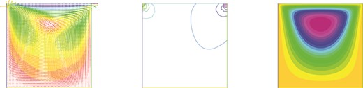
Test 2: (a) The expected value of |$\{ \textbf {u}^N_h\}_n$|. (b) Level-lines of the expected value of |$\{p^N_h\}_n$|. (c) The streamlines of the expected value of |$\{ \textbf {u}^N_h\}_n$|.
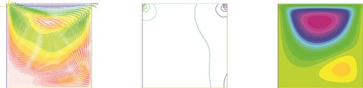
First realization of (a) the velocity |$\{ \textbf {u}^N_h\}_n$|, (b) the pressure |$\{p^N_h\}_n$| and (c) the streamline of |$\{ \textbf {u}^N_h\}_n$|.
Algorithm 4: spatial discretization errors for the velocity |$\{ \textbf {u}^n_{\varepsilon ,h}\}_n$| and pressure |$\{p^n_{\varepsilon ,h}\}_n$|
| |$h$| | |${\pmb {\mathcal {E}}}_{\mathbf {u},0}^N$| | Order | |${\mathcal {E}}_{p,0}^N $| | Order |
|---|---|---|---|---|
| |$1/5$| | 0.018392 | 0.147406 | ||
| |$1/10$| | 0.009083 | 1.0178 | 0.092913 | 0.6658 |
| |$1/20$| | 0.004095 | 1.1493 | 0.052611 | 0.8205 |
| |$1/40$| | 0.002279 | 0.8454 | 0.044723 | 0.2344 |
Standard stabilization method: spatial discretization errors for the velocity |$\{ \textbf {u}^n_{\varepsilon ,h}\}_n$| and pressure |$\{p^n_{\varepsilon ,h}\}_n$|
| |$h$| | |${\pmb {\mathcal {E}}}_{\mathbf {u},0}^N$| | Order | |${\mathcal {E}}_{p,0}^N $| | Order |
|---|---|---|---|---|
| |$1/5$| | 0.037658 | 0.735843 | ||
| |$1/10$| | 0.025586 | 0.5576 | 0.888352 | -0.2717 |
| |$1/20$| | 0.019342 | 0.4036 | 0.579818 | 0.6155 |
| |$1/40$| | 0.011412 | 0.7611 | 0.442691 | 0.3893 |
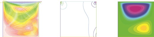
Second realization of (a) the velocity |$\{ \textbf {u}^N_h\}_n$|, (b) the pressure |$\{p^N_h\}_n$| and (c) the streamline of |$\{ \textbf {u}^N_h\}_n$|.
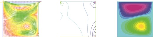
Third realization of (a) the velocity |$\{ \textbf {u}^N_h\}_n$|, (b) the pressure |$\{p^N_h\}_n$| and (c) the streamline of |$\{ \textbf {u}^N_h\}_n$|.
Acknowledgements
After this paper was finished, reference Breit & Dodgson (2019) was brought to our attention by Prof. D. Breit. The finite element method proposed in Breit & Dodgson (2019) is essentially equivalent to Algorithm 2 of this paper although they are different algorithmically.
Funding
National Science Foundation (DMS-1620168 and DMS-2012414 to X.F.; DMS-1620168 and DMS-2012414 to L.V.).
Dedicated to the memory of John W. Barrett
References
