


Abstract
We prove convergence with optimal algebraic rates for an adaptive finite element method for nonlinear equations with strongly monotone operator. Unlike prior works, our analysis also includes the iterative and inexact solution of the arising nonlinear systems by means of the Picard iteration. Using nested iteration, we prove, in particular, that the number of Picard iterations is uniformly bounded in generic cases, and the overall computational cost is (almost) optimal. Numerical experiments confirm the theoretical results.
1. Introduction
In recent years, the analysis of convergence and optimal convergence behaviour of adaptive finite element methods has matured. We refer to the seminal works for some milestones of linear elliptic equations (Dörfler, 1996; Morin et al., 2000; Binev et al., 2004; Stevenson, 2007; Cascon et al., 2008; Feischl et al., 2014), nonlinear problems (Veeser, 2002; Diening & Kreuzer, 2008; Belenki et al., 2012; Garau et al., 2012) and some general abstract framework (Carstensen et al., 2014). Although the interplay between adaptive mesh refinement, optimal convergence rates and inexact solvers has already been addressed and analysed for linear PDEs (e.g., Stevenson, 2007; Arioli et al., 2013a,b; Carstensen et al., 2014) and for eigenvalue problems (Carstensen & Gedicke, 2012), the influence of inexact solvers for nonlinear equations has not been analysed yet. The work by Garau et al. (2011) considers adaptive mesh refinement in combination with a Kačanov-type iterative solver for strongly monotone operators. In the spirit of Morin et al. (2008) and Siebert (2011), the focus is on a plain convergence result of the overall strategy, whereas the proof of optimal convergence rates remains open.
On the other hand, there is a rich body on a posteriori error estimation, which also includes the iterative and inexact solution for nonlinear problems (see, e.g., Ern & Vohralík, 2013). This study aims to close the gap between the numerical analysis (e.g., Carstensen et al., 2014) and the empirical evidence of optimal convergence rates (e.g., Garau et al., 2011; Ern & Vohralík, 2013) by analysing an adaptive algorithm from Congreve & Wihler (2017).
- (O1)|$\boldsymbol A$| is strongly monotone: There exists |$\alpha>0,$| such that\begin{align*}\alpha\,\left\| {{w-v}} \right\|_{\mathcal{H}}^2 \le \operatorname{Re}\,\left\langle {{Aw-Av}\,,\,{w-v}} \right\rangle\quad\text{for all} v,w\in\mathcal{H}. \end{align*}
- (O2) |$\boldsymbol A$| is Lipschitz continuous: There exists |$L>0,$| such that\begin{align*}\left\| {{Aw-Av}} \right\|_{\mathcal{H}^*} \le L\,\left\| {{w-v}} \right\|{\mathcal{H}}\quad\text{for all}\,v,w\in\mathcal{H}. \end{align*}
- (O3) |$\boldsymbol{A}$| has a potential: There exists a Gâteaux differentiable function |$P:\mathcal{H}\to\mathbb{K,}$| such that its derivative |${\rm d}P:\mathcal{H}\to\mathcal{H}^*$| coincides with |$A$|, i.e., for all |$v,w\in\mathcal{H}$|, it holds that(1.2)\begin{align}\left\langle {{Aw}\,,\,{v}} \right\rangle=\left\langle {{{\rm d} P(w)}\,,\,{v}} \right\rangle=\lim_{\substack{r\to 0\\r\in\mathbb{R}}}\frac{P(w+rv)-P(w)}{r}.\end{align}
We note that (O1)–(O2) guarantee that there exists a unique solution |$u^\star \in\mathcal{H}$| to (1.1). The latter is the limit of any sequence of Picard iterates |$u^{n+1} = \varPhi(u^n)$| for all |$n\in\mathbb{N}_0$| with arbitrary initial guess |$u^0\in\mathcal{H}$|, where the nonlinear mapping |$\varPhi:\mathcal{H}\to\mathcal{H}$| is a contraction (see Section 2 for details). The additional assumption (O3) implies that the nonlinear problem (1.1) and its later discretization are equivalently stated as energy-minimization problems (Lemma 5.1). In view of applications, we admit that (O1)–(O2) exclude the |$p$|-Laplacian (Veeser, 2002; Diening & Kreuzer, 2008; Belenki et al., 2012), but cover the same problem class as Garau et al., 2011, 2012; Congreve & Wihler, 2017. For applications of strongly monotone nonlinearities arising in magnetostatics, we also refer to Bruckner et al., 2014.
Based on adaptive mesh refinement of an initial triangulation |$\mathcal{T}_0$|, our adaptive algorithm generates a sequence of conforming nested subspaces |$\mathcal{X}_\ell\subseteq\mathcal{X}_{\ell+1}\subset\mathcal{H}$|, corresponding discrete solutions |$u_\ell\in\mathcal{X}_\ell$| and a posteriori error estimators |$\eta_\ell(u_\ell),$| such that |$\left\| {{u^\star-u_\ell}} \right\|_{\mathcal{H}} \le C_{\rm rel}^\star \,\eta_\ell(u_\ell)\to0$| as |$\ell\to\infty$| at optimal algebraic rate in the sense of certain approximation classes (Cascon et al., 2008; Carstensen et al., 2014; Feischl et al., 2014). Although the plain convergence result from Garau et al. (2011) applies to various marking strategies, our convergence analysis follows the concepts from Cascon et al. (2008), Feischl et al. (2014) and Carstensen et al. (2014), and is hence tailored to the Dörfler marking strategy.
General notation.|$\quad$| Throughout all statements, all constants and their dependencies are explicitly given. In proofs, we may abbreviate the notation by the use of the symbol |$\lesssim$|, which indicates |$\leq$| up to some multiplicative constant that is clear from the context. Moreover, the symbol |$\simeq$| states that both estimates |$\lesssim$| and |$\gtrsim$| hold. If (discrete) quantities are related to some triangulation, this is explicitly stated by the use of appropriate indices, e.g., |$u_\bullet$| is the discrete solution for the triangulation |$\mathcal{T}_\bullet$|, |$v_\circ$| is a generic discrete function in the discrete space |$\mathcal{X}_\circ$|, and |$\eta_\ell(\cdot)$| is the error estimator with respect to the triangulation |$\mathcal{T}_\ell$|.
2. Banach fixpoint theorem
Hence, |$\varPhi:\mathcal{H}\to\mathcal{H}$| is a contraction with Lipschitz constant |$0<q<1$|. According to the Banach’s fixpoint theorem, |$\varPhi$| has a unique fixpoint |$u^\star\in\mathcal{H}$|, i.e., |$u^\star = \varPhi u^\star$|. By definition of |$\varPhi$|, the strong form (1.1) is equivalent to |$u^\star = \varPhi u^\star$|. Overall, (1.1) admits a unique solution.
Thus, the a posteriori computable term |$\left\| {{u^n-u^{n-1}}} \right\|_{\mathcal{H}}$| provides an upper bound for |$\left\| {{u^\star-u^n}} \right\|_{\mathcal{H}}$| as well as a lower bound for |$\left\| {{u^\star-u^{n-1}}} \right\|_{\mathcal{H}}$|.
3. Discretization and a priori error estimation
3.1 Nonlinear discrete problem
First, recall the following well-known Céa-type estimate for strongly monotone operators. We include its proof for the sake of completeness.
Finite dimension concludes that the infimum over all |$w_\bullet \in \mathcal{X}_\bullet$| is, in fact, attained. □
3.2 Linearized discrete problem
Note that the nonlinear system (3.1) can hardly be solved exactly. With the discrete Riesz mapping |$I_\bullet:\mathcal{X}_\bullet\to\mathcal{X}_\bullet^*$| and the restriction |$F_\bullet\in\mathcal{X}_\bullet^*$| of |$F$| to |$\mathcal{X}_\bullet$|, define |$\varPhi_\bullet:\mathcal{X}_\bullet\to\mathcal{X}_\bullet$| by |$\varPhi_\bullet v_\bullet:=v_\bullet-(\alpha/L^2)I_\bullet^{-1}(A_\bullet v_\bullet-F_\bullet)$|. Given |$u_\bullet^{n} \in \mathcal{X}_\bullet$|, we thus compute the discrete Picard iterate |$u_\bullet^{n} := \varPhi_\bullet u^{n-1}_\bullet$| as follows:
(i) Solve the linear system |$(v_\bullet, w_\bullet)_\mathcal{H} = \left\langle {{A u_\bullet^{n-1} - F}\,,\,{v_\bullet}} \right\rangle$| for all |$v_\bullet \in \mathcal{X}_\bullet$|.
(ii) Define |$u_\bullet^{n} := u_\bullet^{n-1} - \frac{\alpha}{L^2} w_\bullet$|.
Finally, we recall the following a priori estimate for the discrete Picard iteration from Congreve & Wihler (2017, Proposition 2.1) and also include its simple proof for the sake of completeness:
With |$\displaystyle \left\| {{u^\star-u_\bullet^n}} \right\|_{\mathcal{H}} \le \left\| {{u^\star-u_\bullet^\star}} \right\|_{\mathcal{H}} + \left\| {{u_\bullet^\star-u_\bullet^n}} \right\|_{\mathcal{H}} \stackrel{(3.3)}\le \left\| {{u^\star-u_\bullet^\star}} \right\|_{\mathcal{H}} + \frac{q^n}{1-q}\,\left\| {{u_\bullet^1-u_\bullet^0}} \right\|_{\mathcal{H}},$| the proof follows from the Céa-type estimate of Lemma 3.1. □
Therefore, boundedness of |$\left\| {{u_\bullet^1-u_\bullet^0}} \right\|_{\mathcal{H}}$| in the a priori estimate of Lemma 3.2 can be guaranteed independently of the space |$\mathcal{X}_\bullet \subset \mathcal{H}$| by choosing, e.g., |$u_\bullet^0:=0$|. If |$\min_{w_\bullet\in\mathcal{X}_\bullet}\left\| {{u^\star-w_\bullet}} \right\|_{\mathcal{H}} = \mathcal{\rm O}(N^{-s})$| for some |$s>0$| and with |$N>0$| being the degrees of freedom associated with |$\mathcal{X}_\bullet$|, this suggests the choice |$n = \mathcal{\rm{O}}(\log N)$| in Lemma 3.2 (see the discussion in Congreve & Wihler, 2017, Remark 3.7). Moreover, we shall see below that the choice of |$u_\bullet^0$| by nested iteration generically leads to |$n = \mathcal{\rm{O}}(1)$| (see Proposition 4.6 below). □
4. Adaptive algorithm
4.1 Basic properties of mesh refinement
Suppose that all considered discrete spaces |$\mathcal{X}_\bullet\subset\mathcal{H}$| are associated with a triangulation |$\mathcal{T}_\bullet$| of a fixed bounded Lipschitz domain |$\varOmega \subset\mathbb{R}^d$|, |$d\ge2$|. Suppose that |$\operatorname{refine}(\cdot)$| is a fixed mesh-refinement strategy.
Given a triangulation |$\mathcal{T}_\bullet$| and |$\mathcal{M}_\bullet \subseteq \mathcal{T}_\bullet$|, let |$\mathcal{T}_\circ := \operatorname{refine}(\mathcal{T}_\bullet,\mathcal{M}_\bullet)$| be the coarsest triangulation, such that all marked elements |$T \in \mathcal{T}_\bullet$| have been refined, i.e., |$\mathcal{M}_\bullet \subseteq \mathcal{T}_\bullet \setminus \mathcal{T}_\circ$|.
We write |$\mathcal{T}_\circ\in\operatorname{refine}(\mathcal{T}_\bullet)$| if |$\mathcal{T}_\circ$| is obtained by a finite number of refinement steps, i.e., there exists |$n\in\mathbb{N}_0$| as well as a finite sequence |$\mathcal{T}_{(0)},\dots,\mathcal{T}_{(n)}$| of triangulations and corresponding sets |$\mathcal{M}_{(j)}\subseteq\mathcal{T}_{(j)}$| such that
|$\mathcal{T}_\bullet = \mathcal{T}_{(0)}$|,
|$\mathcal{T}_{(j+1)} = \operatorname{refine}(\mathcal{T}_{(j)},\mathcal{M}_{(j)})$| for all |$j=0,\dots,n-1$|,
|$\mathcal{T}_\circ = \mathcal{T}_{(n)}$|.
In particular, |$\mathcal{T}_\bullet\in\operatorname{refine}(\mathcal{T}_\bullet)$|. Further, we suppose that refinement |$\mathcal{T}_\circ\in \operatorname{refine}(\mathcal{T}_\bullet)$| yields nestedness |$\mathcal{X}_\bullet\subseteq\mathcal{X}_\circ$| of the corresponding discrete spaces.
In view of the adaptive algorithm (Algorithm 4.3 below), let |$\mathcal{T}_0$| be a fixed initial triangulation. To ease notation, let |$\mathbb{T}:=\operatorname{refine}(\mathcal{T}_0)$| be the set of all possible triangulations that can be obtained by successively refining |$\mathcal{T}_0$|.
4.2 A posteriori error estimator
We suppose the following properties with fixed constants |$C_{\rm stb},C_{\rm red},C_{\rm rel}^\star,C_{\rm drel}^\star \ge 1$| and |$0<q_{\rm red}<1$|, which slightly generalise those axioms of adaptivity of Carstensen et al. (2014):
- (A1) Stability on nonrefined element domains: For all triangulations |$\mathcal{T}_\bullet\in\mathbb{T}$| and |$\mathcal{T}_\circ\in\operatorname{refine}(\mathcal{T}_\bullet)$|, arbitrary discrete functions |$v_\bullet\in\mathcal{X}_\bullet$| and |$v_\circ\in\mathcal{X}_\circ$| and an arbitrary set |$\mathcal{U}_\bullet\subseteq\mathcal{T}_\bullet\cap\mathcal{T}_\circ$| of nonrefined elements, it holds that$$|\eta_\circ(\mathcal{U}_\bullet,v_\circ)-\eta_\bullet(\mathcal{U}_\bullet,v_\bullet)| \le C_{\rm stb}\,\left\| {{v_\bullet-v_\circ}} \right\|_{\mathcal{H}}.$$
- (A2) Reduction on refined element domains: For all triangulations |$\mathcal{T}_\bullet\in\mathbb{T}$| and |$\mathcal{T}_\circ\in\operatorname{refine}(\mathcal{T}_\bullet)$|, and arbitrary |$v_\bullet\in\mathcal{X}_\bullet$| and |$v_\circ\in\mathcal{X}_\circ$|, it holds that$$\eta_\circ(\mathcal{T}_\circ\backslash\mathcal{T}_\bullet,v_\circ)^2 \le q_{\rm red}\,\eta_\bullet(\mathcal{T}_\bullet\backslash\mathcal{T}_\circ,v_\bullet)^2 + C_{\rm red}\,\left\| {{v_\circ-v_\bullet}} \right\|_{\mathcal{H}}^2.$$
- (A3) Reliability: For all triangulations |$\mathcal{T}_\bullet\in\mathbb{T}$|, the error of the discrete solution |$u_\bullet^\star\in\mathcal{X}_\bullet$| to (3.1) is controlled by$$\left\| {{u^\star-u_\bullet^\star}} \right\|_{\mathcal{H}}\le C_{\rm rel}^\star\,\eta_\bullet(u_\bullet^\star).$$
- (A4) Discrete reliability: For all |$\mathcal{T}_\bullet\in\mathbb{T}$| and all |$\mathcal{T}_\circ\in\operatorname{refine}(\mathcal{T}_\bullet)$|, there exists a set |$\mathcal{R}_{\bullet,\circ}\subseteq\mathcal{T}_\bullet$| with |$\mathcal{T}_\bullet\backslash\mathcal{T}_\circ \subseteq \mathcal{R}_{\bullet,\circ}$| as well as |$\#\mathcal{R}_{\bullet,\circ} \le C_{\rm drel}^\star\,\#(\mathcal{T}_\bullet\backslash\mathcal{T}_\circ)$|, such that the difference of the discrete solutions |$u_\bullet^\star \in \mathcal{X}_\bullet$| and |$u_\circ^\star \in \mathcal{X}_\circ$| is controlled by\begin{align*}\left\| {{u_\circ^\star-u_\bullet^\star}} \right\|_{\mathcal{H}} \le C_{\rm drel}^\star\,\eta_\bullet(\mathcal{R}_{\bullet,\circ},u_\bullet^\star). \end{align*}
Suppose the following approximation property of |$u^\star \in \mathcal{H}$|: for all |$\mathcal{T}_\bullet \in \mathbb{T}$| and all |$\varepsilon >0$|, there exists a refinement |$\mathcal{T}_\circ \in \operatorname{refine}(\mathcal{T}_\bullet)$|, such that |$\left\| {{u^\star - u_\circ^\star}} \right\|_{\mathcal{H}} \leq \varepsilon$|. Then, discrete reliability (A4) already implies reliability (A3) (see Carstensen et al., 2014, Lemma 3.4).
We note that (A3)–(A4) are formulated for the noncomputable Galerkin solutions |$u_\bullet^\star\in\mathcal{X}_\bullet$| to (3.1), whereas Algorithm 4.3 below generates approximations |$u_\bullet^{n}\approx u_\bullet^\star\in\mathcal{X}_\bullet$|. The following lemma proves that reliability (A3) transfers to certain Picard iterates.
Combining these estimates, we conclude the proof. □
4.3 Adaptive algorithm
In the sequel, we analyse the following adaptive algorithm which—up to a different a posteriori error estimation based on elliptic reconstruction—is also considered in Congreve & Wihler (2017).
Input: Initial triangulation |$\mathcal{T}_0$|, adaptivity parameters |$0<\theta\le 1$|, |$\lambda>0$| and |$C_{\rm mark}\ge1$|, arbitrary initial guess |$u_0^0\in\mathcal{X}_0$|, e.g., |$u_0^0:=0$|.
Adaptive loop: For all |$\ell=0,1,2,\dots$|, iterate the following Steps (i)–(iii).
(i) Repeat the following Steps (a)–(b) for all |$n=1,2,\dots$|, until |$\left\| {{u_\ell^n-u_\ell^{n-1}}} \right\|_{\mathcal{H}} \le \lambda\,\eta_\ell(u_\ell^n)$|.
(a) Compute discrete Picard iterate |$u_\ell^n = \varPhi_\ell u_\ell^{n-1}\in\mathcal{X}_\ell$|.
(b) Compute refinement indicators |$\eta_\ell(T,u_\ell^n)$| for all |$T\in\mathcal{T}_\ell$|.
(ii) Define |$u_\ell := u_\ell^n \in \mathcal{X}_\ell$| and determine a set |$\mathcal{M}_\ell\subseteq\mathcal{T}_\ell$| of marked elements that have minimal cardinality up to the multiplicative constant |$C_{\rm mark}$| and that satisfy the Dörfler marking criterion |$\theta\,\eta_\ell(u_\ell) \le \eta_\ell(\mathcal{M}_\ell,u_\ell)$|.
(iii) Generate the new triangulation |$\mathcal{T}_{\ell+1} := \operatorname{refine}(\mathcal{T}_\ell,\mathcal{M}_\ell)$| by refinement of (at least) all marked elements |$T\in\mathcal{M}_\ell$| and define |$u_{\ell+1}^0 := u_\ell \in\mathcal{X}_\ell\subseteq\mathcal{X}_{\ell+1}$|.
Output: Sequence of discrete solutions |$u_\ell\in\mathcal{X}_\ell$| and corresponding estimators |$\eta_\ell(u_\ell)$|. □
The following two results analyse the (lucky) breakdown of Algorithm 4.3. The first proposition shows that, if the repeat loop of Step (i) does not terminate after finitely many steps then the exact solution |$u^\star=u_\ell^\star$| belongs to the discrete space |$\mathcal{X}_\ell$|.
This concludes (4.3). □
The second proposition shows that, if the repeat loop of Step (i) does terminate with |$\eta_\ell(u_\ell)=0$|, then |$u_\ell = u^\star$| as well as |$\eta_k(u_k)=0$| and |$u_k=u_k^1=u^\star$| for all |$k>\ell$|.
Suppose (O1)–(O2) for the operator |$A$| as well as stability (A1) and reliability (A3) for the error estimator. If Step (i) in Algorithm 4.3 terminates with |$\eta_\ell(u_\ell)=0$| (or equivalently with |$\mathcal{M}_\ell = \emptyset$| in Step (ii)) for some |$\ell\in\mathbb{N}_0$|, then |$u_k=u^\star$| as well as |$\mathcal{M}_k = \emptyset$| for all |$k \geq \ell$|. Moreover, for all |$k \geq \ell+1$|, Step (i) terminates after one iteration.
Clearly, |$\mathcal{M}_\ell = \emptyset$| implies |$\eta_\ell(u_\ell)=0$|. Conversely, |$\eta_\ell(u_\ell)=0$| also implies |$\mathcal{M}_\ell = \emptyset$|. In this case, Lemma 4.2 yields |$\left\| {{u^\star-u_\ell}} \right\|_{\mathcal{H}}=0$| and hence |$u_\ell=u^\star$|. Moreover, |$\mathcal{M}_\ell = \emptyset$| implies |$\mathcal{T}_{\ell+1} = \mathcal{T}_\ell$|. Nested iteration guarantees |$u_{\ell+1}^1 = \varPhi_{\ell+1} u_{\ell+1}^0 =\varPhi_{\ell+1} u_\ell =\varPhi_{\ell+1} u^\star = u^\star = u_\ell = u_{\ell+1}^0$| and therefore |$\left\| {{u_{\ell+1}^1 - u_{\ell+1}^0}} \right\|_{\mathcal{H}} =0$|. Together with |$\mathcal{T}_{\ell+1}=\mathcal{T}_\ell$|, this implies |$u_{\ell+1} = u_\ell$| and |$\eta_{\ell+1}(u_{\ell+1})=\eta_\ell(u_\ell)=0$|. Hence, for all |$k \geq {\ell+1}$|, Step (i) terminates after one iteration with |$u_k = u^\star$| and |$\mathcal{M}_k =\emptyset$|. □
For the rest of this section, we suppose that Step (i) of Algorithm 4.3 terminates with |$\eta_\ell(u_\ell)>0$| for all |$\ell \in \mathbb{N}_0$|. In this case, we control the number of Picard iterates |$\#{\rm Pic}(\ell)$|.
The constant |$C_{\rm pic}$| depends only on (O1)–(O2), (A1) and (A3).
The proof of Proposition 4.6 employs the following auxiliary result.
This concludes the proof. □
We prove the assertion in two steps.
This contradicts the minimality of |$k$| and concludes |$k \leq n$|.
Linear convergence (see Theorem 5.3 below) proves, in particular, that |$\eta_{\ell}(u_{\ell}) \,{\le} C_{\rm lin} q_{\rm lin}\,\eta_{\ell-1}(u_{\ell-1})$| for all |$\ell\in\mathbb{N}$|. In practice, we observe that |$\eta_{\ell}(u_{\ell})$| is only improved by a fixed factor, i.e., there also holds the converse estimate |$\eta_{\ell-1}(u_{\ell-1}) \le \widetilde C\,\eta_{\ell}(u_{\ell})$| for all |$\ell\in\mathbb{N}$|. Even though, we cannot thoroughly prove this fact, Proposition 4.6 shows that—up to such an assumption—the number of Picard iterations in each step of Algorithm 4.3 is, in fact, uniformly bounded with |$\# {\rm Pic}(\ell)\,{\le} C_{\rm pic}+\frac{1}{{|\!}\log q|}\,\log(\max\{1,\widetilde C\})$|.
4.4 Estimator convergence
In this section, we show that, if Step (i) of Algorithm 4.3 terminates for all |$\ell \in \mathbb{N}_0$|, then Algorithm 4.3 yields |$\eta_\ell(u_\ell)\to0$| as |$\ell\to\infty$|.
We first show that the iterates |$u_\bullet = u_\bullet^n$| of Algorithm 4.3 are close to the noncomputable exact Galerkin approximation |$u_\bullet^\star\in\mathcal{X}_\bullet$| to (3.1) and that the corresponding error estimators are equivalent.
This concludes the proof. □
The following proposition gives a first convergence result for Algorithm 4.3. Unlike the stronger convergence result of Theorem 5.3 below, plain convergence only relies on (O1)–(O2), but avoids the use of (O3).
We prove the assertion in three steps.
Note that |$\lambda < C_\lambda^{-1} \theta$| implies |$\theta'>0$|. Hence, this is the Dörfler marking for |$u_\ell^\star$| with parameter |$0<\theta'<\theta$|. Therefore, Carstensen et al. (2014, Lemma 4.7) proves (4.11).
In particular, we infer that |$\left\| {{u_{\ell+1}^\star-u_\ell^\star}} \right\|_{\mathcal{H}}^2\to0$| as |$\ell\to\infty$|.
Step 3.|$\quad$| According to (4.11) and Step 2, the sequence |$\big(\eta_\ell(u_\ell^\star)\big)_{\ell\in\mathbb{N}_0}$| is contractive up to a non-negative perturbation, which tends to zero. Basic calculus (e.g., Aurada et al., 2012, Lemma 2.3) proves |$\eta_\ell(u_\ell^\star)\to0$| as |$\ell\to\infty$|. Lemma 4.9 guarantees the equivalence |$\eta_\ell(u_\ell^\star)\simeq\eta_\ell(u_\ell)$|. This concludes the proof. □
If the ‘discrete limit space’ |$\mathcal{X}_\infty := \overline{\bigcup_{\ell=0}^\infty\mathcal{X}_\ell}$| satisfies |$\mathcal{X}_\infty = \mathcal{H}$|, possible smoothness of |$A$| guarantees |$\left\| {{u^\star-u_\ell^\star}} \right\|_{\mathcal{H}} + {\rm osc}_\ell(u_\ell^\star)\to0$| as |$\ell\to\infty$| (see the argumentation in Erath & Praetorius, 2016, Proof of Theorem 3). Moreover, |$\mathcal{X}_\infty = \mathcal{H}$| follows either implicitly if |$u^\star$| is ‘nowhere discrete’ or can explicitly be ensured by the marking strategy without deteriorating optimal convergence rates (see Bespalov et al., 2017, Section 3.2). Since |$0<\lambda<C_\lambda^{-1}$|, Lemma 4.9 guarantees estimator equivalence |$\eta_\ell(u_\ell) \simeq \eta_\ell(u_\ell^\star)$|. Overall, such a situation leads to |$\eta_\ell(u_\ell)\to0$| as |$\ell\to\infty$|.
5. Linear convergence
Suppose that |$A$| additionally satisfies (O3). For |$v \in \mathcal{H}$|, we define the energy |$Ev:=\operatorname{Re}(P-F)v$|, where |$P$| is the potential associated with |$A$| from (1.2) and |$F\in\mathcal{H}^*$| is the right-hand side of (1.1). The next lemma generalises Diening & Kreuzer (2008, Lemma 16) and Garau et al. (2012, Theorem 4.1) and states equivalence of the energy difference and the difference in norm.
Together with (5.3), we conclude the proof. □
Lemma 5.1 immediately implies that the Galerkin solution |$u_\bullet^\star\in\mathcal{X}_\bullet$| to (3.1) minimizes the energy |$E$| in |$\mathcal{X}_\bullet$|, i.e., |$E(u_\bullet^\star)\le E(v_\bullet)$| for all |$v_\bullet\in\mathcal{X}_\bullet$|. On the other hand, if |$w_\bullet\in\mathcal{X}_\bullet$| is a minimizer of the energy in |$\mathcal{X}_\bullet$|, we deduce |$E(w_\bullet)=E(u_\bullet^\star)$|. Lemma 5.1 thus implies |$w_\bullet=u_\bullet^\star$|. Therefore, solving the Galerkin formulation (3.1) is equivalent to the minimization of the energy |$E$| in |$\mathcal{X}_\bullet$|.
Next, we prove a contraction property as in Diening & Kreuzer (2008, Theorem 20), Belenki et al. (2012, Theorem 4.7) and Garau et al. (2012, Theorem 4.2) and, in particular, obtain linear convergence of Algorithm 4.3 in the sense of Carstensen et al. (2014).
This concludes the proof. □
6. Optimal convergence rates
6.1 Fine properties of mesh refinement
The proof of optimal convergence rates requires the following additional properties of the mesh-refinement strategy.
- (R1) Splitting property: Each refined element is split in at least 2 and at most in |$C_{\rm son}\ge2$| many sons, i.e., for all |$\mathcal{T}_\bullet \in \mathbb{T}$| and all |$\mathcal{M}_\bullet \subseteq \mathcal{T}_\bullet$|, the refined triangulation |$\mathcal{T}_\circ = \operatorname{refine}(\mathcal{T}_\bullet, \mathcal{M}_\bullet)$| satisfies(6.1)\begin{align}\# (\mathcal{T}_\bullet \setminus \mathcal{T}_\circ) + \# \mathcal{T}_\bullet \leq \# \mathcal{T}_\circ \leq C_{\rm son} \, \# (\mathcal{T}_\bullet \setminus \mathcal{T}_\circ) + \# (\mathcal{T}_\bullet \cap \mathcal{T}_\circ).\end{align}
- (R2) Overlay estimate: For all meshes |$\mathcal{T} \in \mathbb{T}$| and |$\mathcal{T}_\bullet,\mathcal{T}_\circ \in \operatorname{refine}(\mathcal{T})$|, there exists a common refinement |$\mathcal{T}_\bullet \oplus \mathcal{T}_\circ \in \operatorname{refine}(\mathcal{T}_\bullet) \cap \operatorname{refine}(\mathcal{T}_\circ) \subseteq \operatorname{refine}(\mathcal{T})$|, which satisfies\begin{align*}\# (\mathcal{T}_\bullet \oplus \mathcal{T}_\circ) \leq \# \mathcal{T}_\bullet + \# \mathcal{T}_\circ - \# \mathcal{T}. \end{align*}
- (R3) Mesh-closure estimate: There exists |$C_{\rm mesh}>0$| such that the sequence |$\mathcal{T}_\ell$| with corresponding sets of marked elements |$\mathcal{M}_\ell \subseteq \mathcal{T}_\ell$|, which is generated by Algorithm 4.3, satisfies\begin{align*}\# \mathcal{T}_\ell - \# \mathcal{T}_0 \leq C_{\rm mesh} \sum_{j=0}^{\ell -1} \# \mathcal{M}_j. \end{align*}
For the newest vertex bisection (NVB), the mesh-closure estimate (R3) has first been proved for |$d=2$| in Binev et al. (2004) and later for |$d \geq 2$| in Stevenson (2008). Although both works require an additional admissibility assumption on |$\mathcal{T}_0$|, Karkulik et al. (2013) proved that this condition is unnecessary for |$d=2$|. The proof of the overlay estimate (R2) is found in Cascon et al. (2008) and Stevenson (2007). The lower bound of (R1) is clearly satisfied for each feasible mesh-refinement strategy. For NVB, the upper bound of (R1) is easily verified for |$d=2$| with |$C_{\rm son}=4$|, and the proof for general dimension |$d \geq 2$| can be found in Gallistl et al. (2014).
For red-refinement with first-order hanging nodes, the validity of (R1)–(R3) is shown in Bonito & Nochetto (2010). For mesh-refinement strategies in isogeometric analysis, we refer to Morgenstern & Peterseim (2015) for T-splines and to Buffa et al. (2016) and Gantner et al. (2017) for (truncated) hierarchical B-splines.
Using (R1) and the definition of |$\operatorname{refine}(\cdot)$|, an induction argument proves that the lower estimate |$\# (\mathcal{T}_\bullet \setminus \mathcal{T}_\circ) + \# \mathcal{T}_\bullet \leq \# \mathcal{T}_\circ$| in (6.1) holds true for all |$\mathcal{T}_\bullet \in \mathbb{T}$| and arbitrary refinements |$\mathcal{T}_\circ \in \operatorname{refine}(\mathcal{T}_\bullet)$|.
6.2 Approximation class
6.3 Main result
The following theorem is the main result of this work. It proves that Algorithm 4.3 does not only lead to linear convergence, but also guarantees the best possible algebraic convergence rate for the error estimator |$\eta_\ell(u_\ell)$|.
Moreover, there holds |$C_{\rm opt} \,{=}\, C_{\rm opt}'\left\| {{u^\star}} \right\|_{\mathbb{A}_s}$|, where |$C_{\rm opt}'\,{>}\,0$| depends only on |$\mathcal{T}_0$|, |$\theta$|, |$\lambda$|, |$s$|, (A1)–(A4), (O1)–(O2) and (R1)–(R3).
The comparison lemma is found in Carstensen et al. (2014).
The constant |$C_{\rm comp}$| depends only on |$\theta'',s$| and the constants of (A1), (A2) and (A4). □
The proof of Theorem 6.2 follows ideas from Carstensen et al. (2014, Theorem 4.1).
We prove the assertion in three steps.
Step 1.|$\quad$| The implication ‘|$\Longleftarrow$|’ follows by definition of the approximation class, the equivalence |$\eta_\ell(u_\ell^\star)\simeq\eta_\ell(u_\ell)$| from Lemma 4.9 and the upper bound of (R1) (cf. Carstensen et al., 2014, Proposition 4.15). We thus focus on the converse, more important implication ‘|$\Longrightarrow$|’.
Since |$\eta_0(u_0) \simeq \eta_0(u_0^\star) \lesssim \left\| {{u^\star}} \right\|_{\mathbb{A}_s}$|, the latter inequality holds, in fact, for all |$\ell \geq 0$|. Rearranging this estimate, we conclude the proof of (6.5). □
6.4 (Almost) Optimal computational work
We show that Algorithm 4.3 does not only lead to optimal algebraic convergence rates for the error estimator |$\eta_\ell(u_\ell)$|, but also guarantees that the overall cost of the algorithm is asymptotically (almost) optimal.
We suppose that the linear system involved in the computation of each step of the discrete Picard iteration |$u_\ell^n := \varPhi_\ell(u_\ell^{n-1})$|, see Section 3.2, can be solved (e.g., by multigrid) in linear complexity |$\mathcal{\rm{O}}(\# \mathcal{T}_\ell)$|. Moreover, we suppose that the evaluation of |$\left\langle {{A u_\ell^{n-1} -F}\,,\,{v_\ell}} \right\rangle$| and |$\eta_\ell(T,v_\ell)$| for one fixed |$v_\ell \in \mathcal{X}_\ell$| and |$T\in\mathcal{T}_\ell$| is of order |$\mathcal{\rm O}(1)$|. Then, with |$\# {\rm Pic}(\ell)\ge1$| the number of Picard iterates in Step (i) of Algorithm 4.3, we require |$\mathcal{\rm O}(\# {\rm Pic}(\ell) \, \# \mathcal{T}_\ell)$| operations to compute the discrete solution |$u_\ell \in \mathcal{X}_\ell$|.
We suppose that the set |$\mathcal{M}_\ell$| in Step (ii) and the local mesh refinement |$\mathcal{T}_{\ell+1} := \operatorname{refine}(\mathcal{T}_\ell,\mathcal{M}_\ell)$| in Step (iii) of Algorithm 4.3 are performed in linear complexity |$\mathcal{\rm O}(\# \mathcal{T}_\ell)$| (see, e.g., Stevenson, 2007) with |$C_{\rm mark} = 2$| for Step (ii).
Optimal convergence behaviour of Algorithm 4.3 means that, given |$\left\| {{u^\star}} \right\|_{\mathbb{A}_s} < \infty$|, the error estimator |$\eta_\ell(u_\ell)$| decays with rate |$s>0$| with respect to the degrees of freedom |$\mathcal{\rm O}(\# \mathcal{T}_\ell)$| (see Theorem 6.2). Optimal computational complexity would mean that, given |$\left\| {{u^\star}} \right\|_{\mathbb{A}_s} < \infty$|, the error estimator |$\eta_\ell(u_\ell)$| decays with rate |$s>0$| with respect to the computational cost (see Feischl, 2015 for linear problems). Up to some small perturbation, the latter is stated in the following theorem.
There holds |$C_{\rm work} = C_{\rm work}'\,\left\| {{u^\star}} \right\|_{\mathbb{A}_s}$|, where |$C_{\rm work}'>0$| depends only on |$\theta$|, |$\lambda$|, |$s$|, |$\varepsilon$|, (A1)–(A4), (O1)–(O2) and (R1)–(R3), as well as on |$\mathcal{T}_0$|, |$\eta_0(u_0)$| and |$ \# {\rm Pic}(0)$|.
We prove the assertion in three steps.
Rearranging the terms we conclude (6.10) with |$C:=\left(C''' \# \mathcal{T}_0 \, \frac{C_{\rm lin}^{1/s}}{1-q_{\rm lin}^{1/s}} \right)^s\,C_{\rm opt}^{-1}$|.
Step 2.|$\quad$| Let |$s,\delta\,{>}\,0$|. Recall that |$t^{\delta/s} \log(C_0 /t) \,{\to}\, 0$| as |$t \,{\to}\, 0$|. Hence, it follows |$\big(\log(C_0 / \eta_\ell(u_\ell))\big) \eta_\ell(u_\ell)^{\delta/s} \lesssim 1$| as |$\ell \to \infty$|. This implies |$\big(\log(C_0 / \eta_\ell(u_\ell))\big)^{-s} \eta_\ell(u_\ell)^{-\delta} \gtrsim 1$| and results in |$\big(\log(C_0 / \eta_\ell(u_\ell))\big)^{-s} \eta_\ell(u_\ell) \gtrsim \eta_\ell(u_\ell)^{1+\delta}$|, where the hidden constant depends only on |$\delta$|, |$s$|, |$C_0$| and |$\max_{\ell\in\mathbb{N}_0}\eta_\ell(u_\ell)\le C_{\rm mon}\,\eta_0(u_0)$|.
Rearranging the terms concludes the proof. □
7. Optimal convergence of full sequence
In this section, we reformulate Algorithm 4.3 in the sense that the discrete solutions |$(u_\ell)_{\ell\in\mathbb{N}_0}$| correspond to a subsequence |$(\widetilde u_{\ell_k})_{k\in\mathbb{N}_0}$| obtained by the following algorithm, which also accounts for the Picard iterates (see Remark 7.2 below for details). To distinguish between the quantities of Algorithm 4.3 and Algorithm 7.1, we use the tilde for all quantities of Algorithm 7.1, e.g., |$\widetilde\eta_\ell(\widetilde u_\ell)$| is the error estimator corresponding to some |$\widetilde u_\ell\in\widetilde{\mathcal{X}}_\ell$|.
Input: Initial triangulation |$\widetilde{\mathcal{T}}_0:=\mathcal{T}_0$|, adaptivity parameters |$0<\theta\le1$|, |$\lambda\ge0$|, and |$C_{\rm mark}\ge1$|, initial guess |$\widetilde u_{-1}:=0$|.
Adaptive loop: For all |$\ell=0,1,2,\dots$|, iterate the following Steps (i)–(iv).
(i) Compute discrete Picard iterate |$\widetilde u_\ell = \widetilde\varPhi_\ell \widetilde u_{\ell-1}\in\widetilde{\mathcal{X}}_\ell$|.
(ii) Compute refinement indicators |$\widetilde\eta_\ell(T,\widetilde u_\ell)$| for all |$T\in\widetilde{\mathcal{T}}_\ell$|.
(iii) If |$\left\| {{\widetilde u_\ell-\widetilde u_{\ell-1}}} \right\|_{\mathcal{H}} \le \lambda\,\widetilde\eta_\ell(\widetilde u_\ell)$|, do the following Steps (a)–(b).
(a) Determine a set |$\widetilde{\mathcal{M}}_\ell\,{\subseteq}\,\widetilde{\mathcal{T}}_\ell$| of marked elements which has minimal cardinality up to the multiplicative constant |$C_{\rm mark}$| and which satisfies the Dörfler marking criterion |$\theta\,\widetilde\eta_\ell(\widetilde u_\ell) \,{\le}\, \widetilde\eta_\ell(\widetilde{\mathcal{M}}_\ell,\widetilde u_\ell)$|.
(b) Generate the new triangulation |$\widetilde{\mathcal{T}}_{\ell+1} \,{:=}\, \operatorname{refine}(\widetilde{\mathcal{T}}_\ell,\widetilde{\mathcal{M}}_\ell)$| by refinement of (at least) all marked elements |$T\in\widetilde{\mathcal{M}}_\ell$|.
(iv) Else, define |$\widetilde{\mathcal{T}}_{\ell+1} := \widetilde{\mathcal{T}}_\ell$|.
Output: Sequence of discrete solutions |$\widetilde u_\ell\in\widetilde{\mathcal{X}}_\ell$| and corresponding estimators |$\widetilde\eta_\ell(\widetilde u_\ell)$|. □
With |$\ell_{-1}:=-1$| and |$\widetilde{\mathcal{T}}_{-1}:=\mathcal{T}_0$|, define an index sequence |$(\ell_k)_{k\in\mathbb{N}_0}$| inductively as follows:
|$\ell_k > \ell_{k-1}$| is the smallest index such that |$\widetilde{\mathcal{T}}_{\ell_k+1}\neq\widetilde{\mathcal{T}}_{\ell_k}$|;
resp. |$\ell_k=\infty$| if such an index does not exist.
In explicit terms, the indices |$\ell_k$| are chosen such that the mesh is refined after the computation of |$\widetilde u_{\ell_k}$|. Hence, Algorithms 4.3 and 7.1 are related as follows:
|$\widetilde u_{\ell_k} = u_k$| for all |$k\in\mathbb{N}_0$| with |$\ell_k<\infty$|;
|$\widetilde u_{\ell_{k-1}+m} = u_k^m$| for all |$k\in\mathbb{N}_0$| with |$\ell_{k-1}<\infty$| and all |$m\in\mathbb{N}_0$| with |$\ell_{k-1}+m \le \ell_k$|;
|$\widetilde{\mathcal{T}}_\ell = \mathcal{T}_k$| for all |$\ell=\ell_{k-1}+1,\dots,\ell_k$| if |$\ell_k<\infty$|;
|$\widetilde{\mathcal{T}}_\ell = \mathcal{T}_k$| for all |$\ell\ge \ell_{k-1}+1$| if |$\ell_{k-1}<\infty$| and |$\ell_k=\infty$|.
The observations of Remark 7.2 allow to transfer the results for Algorithm 4.3 to Algorithm 7.1. As a consequence of our preceding analysis, we get the following theorem:
Finally, it holds |$\widetilde C_{\rm opt} = C\,C_{\rm opt}$| and |$\widetilde{C}_{\rm work} = C\, C_{\rm work}$|, where |$C_{\rm opt}$| is the constant from Theorem 6.2, |$C_{\rm work}>0$| is the constant from Theorem 6.4 and |$C>0$| depends only on (O1)–(O2), (A3), (R1), |$\mathcal{T}_0$| and |$s$|.
We stick with the notation of Remark 7.2.
Step 1.|$\quad$| Suppose that there exists an index |$\ell\in\mathbb{N}_0$| with |$\left\| {{\widetilde u_\ell-\widetilde u_{\ell-1}}} \right\|_{\mathcal{H}} \le \lambda\,\widetilde\eta_\ell(\widetilde u_\ell)$| and |$\widetilde{\mathcal{M}}_\ell = \emptyset$|. Then, it follows |$\widetilde\eta_\ell(\widetilde u_\ell)=0$|. Proposition 4.5 concludes |$u^\star = \widetilde u_k$|, |$\widetilde{\mathcal{M}}_k = \emptyset$| and |$\widetilde\eta_k(\widetilde u_k)=0$| for all |$k\ge\ell$|. In particular, this proves (7.2)–(7.3) with |$\left\| {{u^\star}} \right\|_{\mathbb{A}_s}<\infty$| for all |$s>0$|.
Step 2. Suppose that there exists an index |$k\in\mathbb{N}_0$| with |$\ell_{k-1}<\infty$| and |$\ell_k=\infty$|. Then, |$\widetilde{\mathcal{T}}_\ell=\widetilde{\mathcal{T}}_{\ell_{k-1}+1}$| for all |$\ell>\ell_{k-1}$|. According to Step 1, we may further assume that |$\left\| {{\widetilde u_\ell-\widetilde u_{\ell-1}}} \right\|_{\mathcal{H}} > \lambda\,\widetilde\eta_\ell(\widetilde u_\ell)$| for all |$\ell>\ell_{k-1}$|. Then, this corresponds to the situation of Proposition 4.4 and hence results in convergence |$\left\| {{u^\star-\widetilde u_\ell}} \right\|_{\mathcal{H}} + \widetilde\eta_\ell(\widetilde u_\ell)\to0$| as |$\ell\to\infty$| and |$\widetilde\eta_\ell(u^\star)=0$| for all |$\ell>\ell_{k-1}$|. Again, this proves (7.2)–(7.3) with |$\left\| {{u^\star}} \right\|_{\mathbb{A}_s}<\infty$| for all |$s>0$|.
Altogether, Theorem 5.3 proves convergence |$\left\| {{u^\star-\widetilde u_\ell}} \right\|_{\mathcal{H}}+\widetilde\eta_\ell(\widetilde u_\ell)\to0$| as |$\ell\to\infty$|.
Step 4.|$\quad$| According to Step 2, we may suppose |$\ell_k<\infty$| for all |$k\in\mathbb{N}_0$|. To show the implication ‘|$\Longleftarrow$|’ of (7.3), it is noted that the right-hand side of (7.3) implies |$\eta_{k}(u_k) \lesssim \big(\#\mathcal{T}_{k} - \# \mathcal{T}_0 +1 \big)^{-s}$| for all |$k\in\mathbb{N}_0$|. Hence, the claim follows from Theorem 6.2.
For |$m>0$|, estimate (4.6) proves |$\widetilde\eta_\ell(\widetilde u_\ell) =\eta_{k}(u_{k}^m) \lesssim \eta_{k-1}(u_{k-1})$|. For |$m=0$|, it holds |$\widetilde\eta_\ell(\widetilde u_\ell)=\eta_{k-1}(u_{k-1})$|. Combining this with the latter estimate, we conclude the proof.
Step 6.|$\quad$| The same argument as in Step 5 in combination with Theorem 6.4 proves (7.4). □
8. Numerical experiments
In this section, we present two numerical experiments in two dimensions to underpin our theoretical findings. In the experiments, we compare the performance of Algorithm 4.3 for
different values of |$\lambda \in \{1, 0.1, 0.01,\ldots,10^{-6}\}$|,
different values of |$\theta \in \{0.2, 0.4,\ldots,1\}$|,
nested iteration |$u_\ell^0 := u_{\ell-1}$| compared with a naive initial guess |$u_\ell^0 := 0$|,
As model problems serve nonlinear boundary value problems similar to those of Garau et al. (2011), Garau et al. (2012), Bruckner et al. (2014) and Congreve & Wihler (2017).
8.1 Model problem
We suppose that the scalar nonlinearity |$\mathbf{\mu}: \varOmega \times \mathbb{R}_{\geq 0} \rightarrow \mathbb{R}$| satisfies the following properties (M1)–(M4), similarly considered in Garau et al. (2012).
- (M1) There exist constants |$0<\gamma_1<\gamma_2<\infty$| such that(8.2)\begin{align}\gamma_1 \le \mathbf{\mu}(x,t) \le \gamma_2 \quad \textrm{for all } x \in \varOmega \text{ and all } t \geq 0.\end{align}
- (M2) There holds |$\mathbf{\mu}(x,\cdot) \in C^1(\mathbb{R}_{\geq 0} ,\mathbb{R})$| for all |$x \in \varOmega$|, and there exist |$0 < \widetilde{\gamma}_1<\widetilde{\gamma}_2<\infty$| such that(8.3)\begin{align}\widetilde{\gamma}_1 \le \mathbf{\mu}(x,t) +2 t \frac{{\mathop{\mathrm{d}{}}}}{{\mathop{\mathrm{d}{t}}}} \mathbf{\mu}(x,t) \le \widetilde{\gamma}_2 \quad \textrm{for all } x \in \varOmega \text{ and all } t \geq 0.\end{align}
- (M3) Lipschitz continuity of |$\mathbf{\mu}(x,t)$| in |$x$|, i.e., there exists |$L_{\mathbf{\mu}}>0$| such that(8.4)\begin{align}| \mathbf{\mu}(x,t) - \mathbf{\mu}(y,t) | \le L_{\mathbf{\mu}} | x - y | \quad \textrm{for all } x,y \in \varOmega \text{ and all } t \geq 0.\end{align}
- (M4) Lipschitz continuity of |$t \frac{{\mathop{\mathrm{d}{}}}}{{\mathop{\mathrm{d}{t}}}} \mathbf{\mu}(x,t)$| in |$x$|, i.e., there exists |$\widetilde{L}_{\mathbf{\mu}}>0$| such that(8.5)\begin{align}\left| t \frac{{\mathop{\mathrm{d}{}}}}{{\mathop{\mathrm{d}{t}}}} \mathbf{\mu}(x,t) - t \frac{{\mathop{\mathrm{d}{}}}}{{\mathop{\mathrm{d}{t}}}} \mathbf{\mu}(y,t) \right| \le \widetilde{L}_{\mathbf{\mu}} | x - y | \quad \textrm{for all } x,y \in \varOmega \text{ and all } t \geq 0.\end{align}
8.2 Weak formulation
Next, we show that |$A$| satisfies (O1)–(O3). For the sake of completeness, we first recall an auxiliary lemma, which is just a simplified version of Liu & Barrett (1996, Lemma 2.1).
Suppose that |$\mathbf{\mu}: \varOmega \times \mathbb{R}_{\geq 0} \rightarrow \mathbb{R}$| satisfies (M1)–(M2). Then, the corresponding operator |$A$| satisfies (O1)–(O3) with constants |$\alpha := \widetilde{\gamma}_1$| and |$L :=\widetilde{\gamma}_2$|.
We prove the assertion in two steps.
Integration over |$\varOmega$| proves strong monotonicity (O1) and Lipschitz continuity (O2).
This concludes |$\left\langle {{\,{\rm d}P(w)}\,,\,{v}} \right\rangle = H^{\prime}(0) = {\int_{{\varOmega}}} \mathbf{\mu}(x,|\nabla w|^2) \, \nabla w \cdot \nabla v \,{\mathop{\mathrm{d}{x}}} \stackrel{(8.7a)}{=} \left\langle {{Aw}\,,\,{v}} \right\rangle$|. □
8.3 Discretization and a posteriori error estimator
The well-posedness of the error estimator requires that the nonlinearity |$\mu(x,t)$| is Lipschitz continuous in |$x$|, i.e., (M3). Then, reliability (A3) and discrete reliability (A4) are proved as in the linear case (see, e.g., Cascon et al., 2008 for the linear case or Garau et al., 2012, Theorem 3.3 and Garau et al., 2012, Theorem 3.4, respectively, for strongly monotone nonlinearities).
The verification of stability (A1) and reduction (A2) requires the validity of a certain inverse estimate. For scalar nonlinearities and under the assumptions (M1)–(M4), the latter is proved in Garau et al. (2012, Lemma 3.7). Using this inverse estimate, the proof of (A1) and (A2) follows as for the linear case (see, e.g., Cascon et al., 2008, for the linear case or Garau et al., 2012, Section 3.3, for scalar nonlinearities). We note that the necessary inverse estimate is, in particular, open for nonscalar nonlinearities. In any case, the arising constants in (A1)–(A4) depend also on the uniform shape regularity of the triangulations generated by newest vertex bisection.
8.4 Experiment with known solution
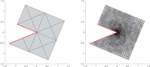
Experiment with known solution from Section 8.4: |$Z$|-shaped domain |$\varOmega \subset \mathbb{R}^2$| and the initial mesh |$\mathcal{T}_0$| (left), and with NVB adaptively generated mesh |$\mathcal{T}_{19}$| with |$5854$| elements (right). |$\Gamma_D$| is visualized by a thick red line.
Our empirical observations are the following: Due to the singular behaviour of |$u^\star$|, uniform refinement leads to a reduced convergence rate |$\mathcal{\rm O}(N^{-\beta/2})$| for both, the energy error |$\left\| {{\nabla u^\star - \nabla u_\ell}} \right\|_{L^2(\varOmega)}$| as well as the error estimator |$\eta_\ell (u_\ell)$|. On the other hand, the adaptive refinement of Algorithm 4.3 regains the optimal convergence rate |$\mathcal{\rm O}(N^{-1/2})$|, independently of the actual choice of |$\theta \in \{0.2, 0.4, 0.6, 0.8\} $| and |$\lambda \in \{1, 0.1, 0.01, \ldots, 10^{-6}\}$| (see Figs 2–4). Throughout, we compare the performance of the iterative solver for naive initial guess |$u_\ell^0:=0$| as well as nested iteration |$u_\ell^0:=u_{\ell-1}$|: The larger the |$\it \lambda$|, the stronger is the influence on the convergence behaviour (see Fig. 4). Moreover, Fig. 5 shows the number of Picard iterations for |$\theta\in\{0.2, 0.8\}$| and |$\it \lambda \in \{\rm 0.1, 0.01, \ldots, 10^{-6}\}$|. As expected from Remark 3.3, for the naive initial guess |$u_\ell^0:=0$|, the number of Picard iterations grows logarithmically with the number of elements |$\#\mathcal{T}_\ell$|, whereas we observe a bounded number of Picard iterations for nested iteration |$u_\ell^0:=u_{\ell-1}$| (cf. Proposition 4.6 respectively Remark 4.8).
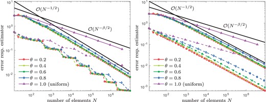
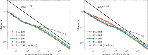
Experiment with known solution from Section 8.4: Convergence of |$\eta_\ell(u_\ell)$| (solid lines) and |$\left\| {{\nabla u^\star - \nabla u_\ell}} \right\|_{L^2(\varOmega)}$| (dashed lines) for |$\lambda = 0.1$| and different values of |$\theta\in\{0.2,\dots, 1\}$|, where we compare naive initial guesses |$u_\ell^0 := 0$| (left) and nested iteration |$u_\ell^0 := u_{\ell-1}$| (right).
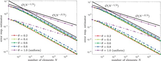
Experiment with known solution from Section 8.4: Convergence of |$\eta_\ell(u_\ell)$| (solid lines) and |$\left\| {{\nabla u^\star - \nabla u_\ell}} \right\|_{L^2(\varOmega)}$| (dashed lines) for |$\lambda = 10^{-5}$| and different values of |$\theta\in\{0.2,\dots, 1 \}$|, where we compare naive initial guesses |$u_\ell^0 := 0$| (left) and nested iteration |$u_\ell^0 := u_{\ell-1}$| (right).
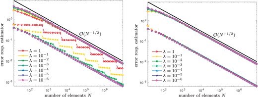
Experiment with known solution from Section 8.4: Convergence of |$\eta_\ell(u_\ell)$| (solid lines) and |$\left\| {{\nabla u^\star - \nabla u_\ell}} \right\|_{L^2(\varOmega)}$| (dashed lines) for |$\theta = 0.2$|, and different values of |$\lambda\in\{1,0.1, 0.01,\dots, 10^{-6} \}$|, where we compare naive initial guesses |$u_\ell^0 := 0$| (left) and nested iteration |$u_\ell^0 := u_{\ell-1}$| (right).
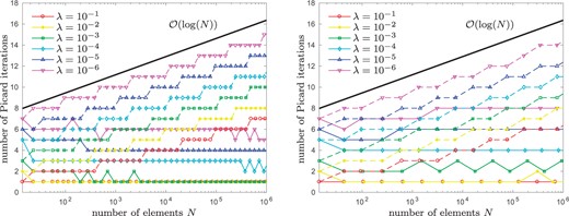
Experiment with known solution from Section 8.4: Number of Picard iterations used in each step of Algorithm 4.3 for different values of |$\lambda\in\{0.1,\dots, 10^{-6} \}$| and |$\theta = 0.2$| (left) as well as |$\theta = 0.8$| (right). As expected, we observe logarithmic growth for naive initial guesses |$u_\ell^0 := 0$| (dashed lines); see Remark 3.3. On the other hand, nested iteration |$u_\ell^0 := u_{\ell-1}$| (solid lines) leads to a bounded number of Picard iterations (see Remark 4.8).
8.5 Experiment with unknown solution
We consider the Z-shaped domain |$\varOmega \subset \mathbb{R}^2$| from Fig. 1 (left) and the nonlinear Dirichlet problem (8.1) with |$\Gamma=\Gamma_D$| and constant right-hand side |$f\equiv1$|, where |$\mu(x, |\nabla u^\star|^{2}) = 1+ \arctan(|\nabla u^\star|^2)$|. According to Congreve & Wihler (2017, Example 1), there holds (O1)–(O2) with |$\alpha = 1$| and |$L = 1+\sqrt{3}/2 + \pi/3$|.
Because the exact solution is unknown, our empirical observations are concerned with the error estimator only (see Figs 6–9). Uniform mesh refinement leads to a suboptimal rate of convergence, whereas the use of Algorithm 4.3 regains the optimal rate of convergence. The latter appears to be robust with respect to |$\theta \in \{0.2,\dots, 0.8\}$| as well as |$\lambda \in \{1, 0.1,\ldots ,10^{-5}\}$|. Although naive initial guesses |$u_\ell^0:=0$| for the iterative solver lead to a logarithmic growth of the number of Picard iterations, the proposed use of nested iteration |$u_\ell^0 := u_{\ell-1}$| again leads to bounded iteration numbers.
Experiment with unknown solution from Section 8.5: Convergence of |$\eta_\ell(u_\ell)$| for |$\lambda = 0.1$| and |$\theta\in\{0.2,\dots, 1\}$|, where we compare naive initial guesses |$u_\ell^0 := 0$| (left) and nested iteration |$u_\ell^0 := u_{\ell-1}$| (right).
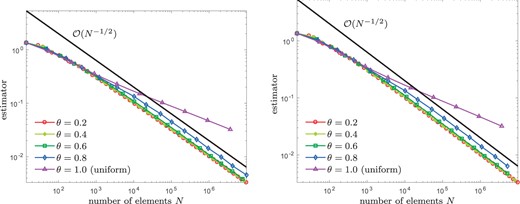
Experiment with unknown solution from Section 8.5: Convergence of |$\eta_\ell(u_\ell)$| for |$\lambda = 10^{-5}$| and |$\theta\in\{0.2,\dots, 1\}$|, where we compare naive initial guesses |$u_\ell^0 := 0$| (left) and nested iteration |$u_\ell^0 := u_{\ell-1}$| (right).
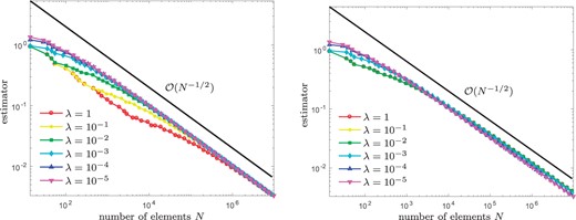
Experiment with unknown solution from Section 8.5: Convergence of |$\eta_\ell(u_\ell)$| for |$\theta = 0.2$| and |$\lambda\in\{1,0.1, 0.01,\dots, 10^{-5} \}$|, where we compare naive initial guesses |$u_\ell^0 := 0$| (left) and nested iteration |$u_\ell^0 := u_{\ell-1}$| (right).
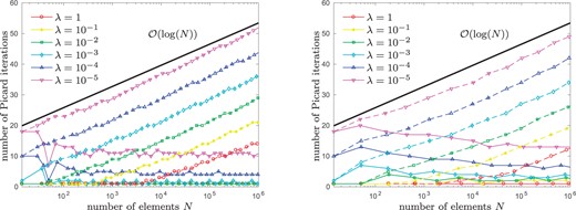
Experiment with unknown solution from Section 8.5: Number of Picard iterations used in each step of Algorithm 4.3 for different values of |$\lambda\in\{1, 0.1,\dots, 10^{-5} \}$| and |$\theta = 0.2$| (left) as well as |$\theta = 0.8$| (right). As expected, we observe logarithmic growth for naive initial guesses |$u_\ell^0 := 0$| (dashed lines) as well as a bounded number of Picard iterations for nested iteration |$u_\ell^0 := u_{\ell-1}$| (solid lines).
9. Conclusions
In this article, we have analysed an adaptive finite element method (FEM) proposed in Congreve & Wihler (2017) for the numerical solution of quasi-linear partial differential equations (PDEs) with strongly monotone operators. Conceptually based on the residual error estimator and the Dörfler marking strategy, the algorithm steers the adaptive mesh refinement and the iterative solution of the arising nonlinear systems by means of a simple fixed point iteration, which is adaptively stopped if the fixed point iterates are sufficiently accurate. In the spirit of Carstensen et al. (2014), the numerical analysis is given in an abstract Hilbert space setting that (at least) covers conforming first-order FEM and certain scalar nonlinearities (Garau et al., 2012).
We prove that our adaptive algorithm guarantees convergence of the finite element solutions to the unique solution of the PDE at optimal algebraic rate for the error estimator (which, in usual applications, is equivalent to energy error plus data oscillations, Garau et al., 2012). Employing nested iterations, we prove that the number of fixed point iterations per mesh is bounded logarithmically with respect to the improvement of the error estimator. As a consequence, we thus prove that the adaptive algorithm is not only convergent at optimal rate with respect to the degrees of freedom, but also at (almost) optimal rate with respect to the computational work.
Numerical experiments for quasi-linear PDEs in |$H^1_0(\varOmega)$| confirm our theory and underline the performance of the proposed adaptive strategy, where each step of the considered fixed point iteration requires only the numerical solution of one linear Poisson problem. In the present work, the iterative and inexact solution of these linear problems is not considered, but it can be included into the analysis (Haberl, yet unpublished).
Overall, this study appears to be the first that guarantees optimal convergence for an adaptive FEM with iterative solver for nonlinear PDEs. Open questions for future research include the following: Is it possible to generalise the numerical analysis to other type of error estimators (e.g., estimators based on equilibrated fluxes, Ern & Vohralík, 2013) as well as higher-order and/or nonconforming FEM (see, e.g., Congreve & Wihler, 2017,, for numerical experiments)? Is it possible to treat nonscalar nonlinearities?
Funding
Austria Science Fund (FWF) through the research project Optimal adaptivity for BEM and FEM-BEM coupling (P27005 to A.H., D.P.) and the research project Optimal isogeometric boundary element methods (P29096 to D.P., G.G.); the FWF doctoral school Nonlinear PDEs funded (W1245 to D.P., G.G.); Vienna Science and Technology Fund (WWTF) through the research project Thermally controlled magnetization dynamics (MA14-44 to B.S., D.P.).
References
Footnotes
1 It is necessary to demand |$\ell\ge\ell_0$|. Indeed, the finitely many estimator values |$\widetilde\eta_\ell(\widetilde u_\ell)$| for |$\ell<\ell_0$| are obviously bounded by a constant. However, this constant does not depend on the constants on which |$\widetilde C_{\rm opt}$| resp. |$\widetilde C_{\rm work}$| depend.
