


Abstract
A new numerical framework is developed to solve general nonlinear and nonlocal PDEs on complicated two-dimensional domains. This enables the solution of a wide range of both steady and time-dependent problems on nonstandard geometries, as well as providing the ability to impose nonlinear and nonlocal boundary conditions (typical of those arising in the modelling of physical phenomena) in a flexible and automated way. This spectral element methodology, which we called MultiShape, is compatible with other state-of-the-art numerical methods, such as differential–algebraic equation solvers and optimization algorithms. MultiShape is an open-source Matlab library, in which the numerical implementation is designed to be user-friendly: the problem set-up and computations are done automatically through intuitive operator definitions and notation. Validation tests are presented, before we showcase the power and versatility of MultiShape with three motivating examples in Dynamic Density Functional Theory and PDE-constrained optimization.
1. Introduction
Many problems in the applied sciences, including biology, chemical engineering and physics, can be described by (integro-) partial differential equation (PDE) models. These include wide-ranging applications of industrial relevance, including those in drug delivery Peppas & Narasimhan (2014), manufacturing (Jaluria, 2018, Chapter 2) and the food industry Erdogdu et al. (2017). Often in these applications, such models need to be solved on complicated domains, to include relevant features of the problem setup, for example, in microfluidics Bridle et al. (2014) and milling processes in the pharmaceutical industry Seibert et al. (2019). Therefore, efficient numerical methods for solving integro-PDEs on complicated domains are of ever-increasing interest to academic and industrial communities Lozinski & Chauvière (2003); Lozinski et al. (2003); Canuto et al. (2007); Zhu & Kopriva (2009a); Rao (2010); Fakhar-Izadi & Dehghan (2014).
Perhaps the most popular numerical scheme for such problems is the finite element method (FEM) Brenner & Scott (2008), which is both an active area of applied mathematics research and frequently used in a wide range of applications Rao (2010), with several commercial and open-source software solutions available, such as FEniCS Smith (2009); Logg et al. (2012); Alnæs et al. (2015). However, for a large class of PDE models, there is another effective numerical method—the pseudospectral method—which, for modelling problems that involve nonlocal phenomena, can be more efficient and accurate than the FEM for a comparable computational cost. We are particularly interested in applications in which nonlocal phenomena enter the model through, for example, fractional operators or convolution integrals, the latter of which we focus on here. For these models, the FEM becomes computationally expensive because one of its key advantages, the frequently-obtained sparse matrix structure, is generally lost. Pseudospectral methods, however, do not rely on sparsity to reduce computational cost, and nonlocal terms can be treated without significant additional complexity. Moreover, pseudospectral methods exhibit exponential convergence in the number of collocation points for analytic functions and can exploit any smoothness of the PDE solution (Boyd, 2001, Chapter 1). For many models that include diffusion and sufficiently ‘nice’ nonlocal interactions, smooth solutions can be expected, even if such results have not yet been rigorously proven. Any potential such proofs are expected to be highly challenging; for example, the PDEs studied in this work are closely related to nonlinear McKean–Vlasov equations, which have recently been shown not to have a unique equilibrium in certain parameter regimes, even with periodic boundary conditions Carrillo et al. (2020).
In Nold et al. (2017), a pseudospectral scheme has been introduced to efficiently solve nonlocal PDEs, including complicated nonlocal boundary conditions on simple domains. The authors provided an open-source software implementation of their method, 2DChebClass, which applies to 1D problems and simple domains in two dimensions, such as rectangles, wedges (sections of an annulus, in polar coordinates) and semi-infinite boxes. Features of this implementation include the straightforward computation of convolution integrals and the user-friendly implementation of complicated, often nonlocal, boundary conditions, which cannot easily be tackled by standard methods, such as boundary bordering (see e.g., (Trefethen, 2000, Chapter 7) and (Boyd, 2001, Chapter 6)).
A natural extension of pseudospectral methods is the spectral element method (SEM), which can be seen as combining a pseudospectral method with a higher-order FEM. We note that the methods described here share strong similarities with (nonoverlapping) domain decomposition methods; see (Boyd, 2001, Chapter 22) for a pseudospectral viewpoint and Toselli & Widlund (2005) for a more general overview. The basis functions used by SEM, such as Chebyshev or Lagrange polynomials, are typically of higher order than those used in FEM. Additionally, SEM generally uses Chebyshev–Lobatto collocation grids on each element. At the intersections between the elements, continuity is enforced by imposing matching conditions, for example, continuity of the solution and its first derivative normal to the intersection, for PDE problems that are second-order in space; see (Boyd, 2001, Chapter 22). There are a number of different, but related, SEMs. First, one could consider the strong form of the PDE and apply matching conditions on the intersections of the elements directly, as previously described. This is called the patching method, and was first introduced by Orszag (1980). Second, there is the Galerkin SEM that solves the weak form of a PDE model, and was pioneered by Patera (1984) using Chebyshev polynomials as basis functions, and later adapted to Lagrange polynomials by Komatitsch & Vilotte (1998), which is now the standard choice (Boyd, 2001, Chapter 22). As shown in Funaro (1986), for elliptic PDEs this approach is essentially equivalent to the patching formulation. A third method for solving a PDE using SEM is based on overlapping elements and was introduced by Morchoisne (1984). In the present work, we apply the patching method.
SEMs have been applied to solve a range of problems. Some of the earlier applications were in (classical) fluid dynamics (see (Canuto et al., 1988, Chapter 13) and (Canuto et al., 2007, Chapter 5)) and geosciences Komatitsch & Vilotte (1998); Fichtner et al. (2009). Further applications of SEM include fractional PDEs Lischke et al. (2019), the equations of relativity Pfeiffer et al. (2003); Grandclément & Novak (2009), financial modelling Zhu & Kopriva (2009a,b, 2010) and optimal control problems with PDE constraints Chen et al. (2008); Zhou & Yang (2011); Chen & Huang (2017). Often SEM is applied as a higher-order FEM, using a large number of elements with low degree polynomials. However, some work has been done on domain decomposition and ‘multidomain’ methods, e.g., Pfeiffer et al. (2003), that actively apply SEM to describe complicated domains using a smaller number of elements and higher degree polynomials. Examples of these include hemodynamics, flow in aircraft engines or around aerofoils (Canuto et al., 2007, Chapter 5) and other obstacles Lozinski et al. (2003), flows in petroleum reservoirs Taneja & Higdon (2018), seismic waves Komatitsch & Vilotte (1998); Fichtner et al. (2009) and sound propagation Lin (1998). While most existing work does not include nonlocal integral terms, some advances have been made; see e.g., Lozinski et al. (2003); Zhu & Kopriva (2009a); Fakhar-Izadi & Dehghan (2014, 2015). These works consider different, mostly one-dimensional, integral terms, which were tackled in the context of the (weak form) Galerkin SEM formalism, using either Gaussian quadrature or Fast Fourier Transforms (FFTs), the latter introducing requirements on the solution’s spatial periodicity, which is usually treated with an artificial truncation of the physical domain. Additionally, the chosen boundary conditions do not involve convolution integral terms, unlike those for the problems considered here.
The present work develops a multidomain SEM for two-dimensional problems, called MultiShape,1 including an open-source software package Roden et al. (2024), which is able to solve various (integro-)PDE problems on complicated domains. This implementation includes the application of complicated boundary conditions, such as (nonlinear, nonlocal) no-flux conditions, as well as the efficient solution of integro-PDEs, involving the evaluation of convolution integrals. For the problems considered in this paper, this is a significant improvement to the approaches taken in the aforementioned works. The work follows from the pseudospectral code library 2DChebClass Nold et al. (2017), extending this framework to a SEM, with minimal additional effort for the user. The flexibility of the method is illustrated by a range of numerical examples in Sections 3 and 4, demonstrating one of the main advantages of the implementation: its compatibility with various other numerical methods such as standard ordinary differential equation (ODE) and state-of-the-art optimization algorithms. We also demonstrate its flexibility with respect to the choice of collocation points. In line with previous work, see Nold et al. (2017); Aduamoah et al. (2022), we present examples that originate from Dynamic Density Functional Theory (DDFT), which describes dynamic properties of systems involving particles suspended in a fluid. Applications of this theory range from mathematical biology, such as in bird flocking or bacteria dynamics Menzel et al. (2016), through medicine, such as in drug delivery Fang et al. (2005), to social sciences, such as in opinion dynamics Goddard et al. (2022). In DDFT, the usual way to treat complex geometries is to impose steep potential gradients in parts of the domain, e.g., to model flow through a constriction Zimmermann et al. (2016), or around obstacles Rauscher et al. (2007); Almenar & Rauscher (2011), which can be computationally expensive due to large gradients in the system. Here, we demonstrate that SEMs are a valuable alternative to this method and solutions to DDFT-like problems on complicated domains using SEM are illustrated in Section 4.
1.1 Novelty
In summary, this work makes the following significant contributions:
A new open-source software package (available online Roden et al. (2024)) for the solution of a broad range of (integro-)PDE problems on complicated domains.
A straightforward interface with other numerical schemes, including differential–algebraic equation solvers and optimization algorithms, with problem set-ups being domain-independent, and re-solving on a new domain requiring little additional effort.
A user-friendly set-up, compatible with the existing 2DChebClass library, easily adapted to new model problems and pseudospectral bases.
The easy application of naturally-arising complicated, nonlinear, nonlocal boundary conditions, which do not have to be determined in a problem-specific way.
Automated constructions of multishapes, whose elements can be defined by a combination of Cartesian and polar coordinates.
Novel methods for the efficient evaluation of convolution integrals, easily applicable to a wide range of kernels.
We note that none of these features were previously available in 2DChebClass, or, to our knowledge, any other open-source SEM package.
1.2 Structure of paper
The paper is structured as follows: in Section 2, the numerical method is introduced in detail. In Section 3 the code is validated with a range of numerical tests, including the Poisson and wave equations, and a Poisson control problem. Section 4 introduces three applications considered in detail: an equilibrium model, an integro-PDE model for particle dynamics and a PDE-constrained control problem. Furthermore, the numerical methods that are used in combination with SEM are introduced. Finally, we close with some remarks in Section 5.
2. MultiShape
In this section, we introduce a general model problem, and describe the structure of and numerical methods utilized in MultiShape. This includes the methods of discretization, differentiation, interpolation, integration and convolution, which are used in the solution process of a user-supplied nonlinear, nonlocal PDE defined on a complicated two-dimensional domain.
2.1 Motivation
The MultiShape framework applies to a broad range of PDE models, some of which are introduced in Sections 3 and 4. A general time-dependent problem is presented in the following, and time-independent PDEs as well as integral equations can also be tackled with MultiShape. Let |$\varOmega \subset \mathbb{R}^{2}$| be a spatial domain with |$\partial \varOmega $| denoting its boundary. Additionally, let |$0\leq t<T$| denote time. We consider a time-dependent PDE for the unknown |$u: \varOmega \times [0,T) \to \mathbb{R}$| of the general form
where |$f$| is a suitably well-behaved function, and, in general, may depend on the unknown |$u$|, and its derivatives and functionals. Note that functional dependence on |$u$| can be nonlinear and nonlocal, an example of which is presented below. Additionally, |$\varGamma $| is a boundary operator defining the behaviour of |$u$| on |$\partial \varOmega $| (which can comprise Dirichlet, Neumann or general Robin conditions) and |$u_{0}$| is suitably nice initial data.
Note that the physically-motivated PDE models from DDFT considered in Section 4 have an inherent gradient flow structure, so that |$f(u):= -\nabla \cdot \mathfrak j(u)$| and |$\varGamma (u):= \mathfrak j(u) \cdot \vec n$|. In particular, one can solve complicated PDEs that have nonlinear, nonlocal fluxes, such as
with given vector-valued functions |$\vec w$|, |$\vec K$|, which also enter the boundary conditions. Note that fields |$\vec w$|, |$\vec K$| are often conservative, i.e., can be written as the gradient of a potential, as is the case for the problems posed in Section 4. Given that nonlocal convolution terms enter both the PDE model and boundary conditions, standard methods such as FEMs are difficult to apply efficiently, since one is unable to exploit sparse matrix structures that typically arise from FEM discretizations, as discussed in the Introduction. Since solutions to PDEs of this form are generally expected to be smooth, one can instead exploit the advantages from SEMs that do not rely on matrix sparsity to be efficient.
2.1.1 Matching conditions
The domain in MultiShape is constructed by discretizing a complicated two-dimensional domain into individual shape elements. We solve the strong form of (2.1) on each of the elements, while matching conditions (patching) are applied at the intersection between two elements, and the PDE boundary conditions are applied on the multishape domain boundary.
For a second-order (in space) PDE of the form (2.1), the matching conditions between elements are
where |$\partial \varOmega _{i,j}$| denotes the intersection boundary between elements |$e_{i}$| and |$e_{j}$|, |$i,j = 1,...,n_{e}$| (which may be empty), and quantities of the form |$f_{i}$| denote the value of |$f$| on element |$i$|. The minus sign in the second matching condition arises due to the opposite orientation of (outward) normals for adjoining elements.
If the PDE problem has gradient flow structure, then, in line with work on SEM for (classical) fluid dynamics problems, e.g., (Canuto et al., 2007, Chapter 5), it is a natural choice to match the flux |$\mathfrak{ \vec j}(u)$| at the intersection of two elements, as compared to directly matching the first derivative of |$u$|. This approach will be taken in the physically motivated example problems solved in Section 4, but note that the two approaches are essentially equivalent. The second matching condition is then replaced by
2.2 Class methods
MultiShape is an object oriented library for solving strong form PDEs defined on arbitrarily shaped physical domains divided into multiple sub-elements (quadrilaterals, annuli, discs and wedges). A multishape domain is defined by a number |$n_{e}$| of these simple elements (shapes), denoted by |$e_{i}$|, |$i = 1,...,n_{e}$|. In the present work, quadrilateral and wedge (section of an annulus) elements can be combined to construct the multishape domain (a discretization of the problem-specific physical domain); see Fig. 1 for an illustration. This can be straightforwardly extended to other shapes that can be mapped (conformally) from/to the unit square (i.e., those used in standard pseudospectral approaches).
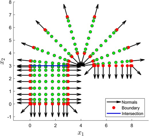
A multishape consisting of a quadrilateral and a wedge element. Displayed are collocation points, highlighted boundary points, the intersection boundary between the two shapes and outward unit normal vectors.
The PDE solver inside MultiShape is based on the existing solver in the library 2DChebClass Nold et al. (2017), extended to the solution of strong form PDEs via the patching method. The choice to solve the strong form of a PDE model and the use of a patching method in MultiShape is motivated by the fact that 2DChebClass provides a strong solution of a PDE on the individual elements. It is also advantageous for the end user, since the weak form of the PDE problem does not have to be derived in order to use this method; the PDE can be inputted directly as stated, e.g., as in Section 2.3.
The new MultiShape implementation aims to be intuitive for both new and 2DChebClass users. In order to elucidate the PDE solution process performed by MultiShape we outline some of the features that are carried forward from 2DChebClass, and which are explained in detail in Nold et al. (2017). In this subsection, we describe the numerical methods utilized in MultiShape’s implementation in Matlab, such as the construction of differentiation and interpolation matrices, integration vectors, convolution operators and the application of intersection conditions.
The implementation of first (gradient, divergence, curl), second (Laplacian) and, optionally, higher-order differentiation matrices are constructed automatically on the discretized shape. These operators are constructed on the computational domain |$[-1,1]^{2}$| for each element and then mapped onto the physical domain using (the inverse of) a bi-linear map, making it easy to define operators on different physical domains (Boyd, 2001, Chapter 22). The interpolation polynomial on an element is defined using barycentric Lagrange interpolation Berrut & Trefethen (2004). For the evaluation of integrals, Clenshaw–Curtis quadrature Clenshaw & Curtis (1960) is applied. For further details on the pseudospectral implementation in 2DChebClass, we refer to Nold et al. (2017).
While many of the key quantities (derivative, interpolant, convolution and so on) can be computed on the individual elements first, a key part of the implementation is that all operators can be applied to the whole interior of the multishape domain simultaneously, which is described in the following. Note that, since quadrilateral and wedge elements are defined in two different coordinate systems, Cartesian and polar, the corresponding operators are defined in terms of two different coordinate systems as well. Most computations, such as differentiation, integration and interpolation, are defined locally on each element, while global operations, such as convolution integrals, are defined on the whole multishape domain. Boundary and intersection matching conditions are treated as separate algebraic constraints of the problem, so these parts of the domain are not a concern when constructing discretizations of the PDE operators for the interior of the domain.
2.2.1 Discretization
Whilst Fourier pseudospectral methods are well suited to periodic problems, such domains are not directly applicable in a spectral element setting. Hence, here we restrict ourselves to discussing the case in which each dimension of a square, |$[-1,1]$|, is discretized using Gauss–Lobatto–Chebyshev collocation points, defined as
for |$i = 0,1,...,N-1$|. Note that, in Section 3.4 we also consider the Legendre–Gauss–Lobatto (LGL) collocation method, which demonstrates the flexibility of the MultiShape approach. However, for clarity, we focus on Chebyshev collocation in the following discussion. In the two-dimensional domain |$[-1,1]^{2}$|, Kronecker products are used to create a two-dimensional grid in the standard way (Trefethen, 2000, Chapter 7). As above, the domain |$[-1,1]^{2}$| is referred to as the computational domain and, using a bi-linear map, it can be associated with a quadrilateral (in the case of 2DChebClass, only a rectangular box is provided by default) or wedge element, which is referred to as the physical domain (Boyd, 2001, Chapter 22). Note that for wedge elements, both the computational and physical domain are defined in polar coordinates.
Discretizing a function |$f$| on a multishape domain is done by discretizing |$f$| on each element individually through 2DChebClass, and stacking the resulting vectors into a vector of size |$M \times 1$|. Here |$M = \sum _{i=1}^{n_{e}} N^{(i)}_{1} N^{(i)}_{2}$|, where |$N^{(i)}_{1}$|, |$N^{(i)}_{2}$| are the number of points for element |$e_{i}$| in the (computational domain) |$x_{1}$| and |$x_{2}$| directions, respectively, and |$n_{e}$| is again the number of elements in the multishape. The resulting discretized function is
where |$\mathbf f_{i}$| is an |$N_{1}^{(i)}N_{2}^{(i)} \times 1$| vector, for |$i = 1,..., n_{e}$|. The same approach is taken when constructing the integration vector, approximating integration on the whole multishape domain, which is a row vector of size |$1 \times M$|.
2.2.2 Differentiation
The gradient, divergence and Laplacian operators for a multishape are constructed by computing the operators locally on each individual element, using 2DChebClass and arranging them in a (sparse) block diagonal matrix, as demonstrated below for an operator |$D$| acting on a function (vector) |$\mathbf f$|:
Note that empty blocks in the above denote zeros. Computations can then be carried out directly on the multishape, instead of on each element individually, since the stacking ensures that the order of elements is preserved. A matrix |$D_{i}$| corresponding to element |$e_{i}$| is applied only to |$\mathbf f_{i}$|, corresponding to the same element, within the matrix–vector multiplication. Note that |$D_{i}$| and |$D_{j}$| could be defined in two different coordinate systems, depending on whether |$e_{i}$| and |$e_{j}$| are quadrilateral or wedge elements.
2.2.3 Interpolation
Interpolating a function |$f$| from one grid onto another is another crucial feature of the MultiShape implementation. Accurate interpolation is relevant for plotting of results, computation of convolutions with finite support and evaluation of quantities on subdomains, as well as comparing results evaluated on different grids. Many of these applications only require the interpolation matrices in computational space |$[-1,1]^{2}$| for each element individually, which can simply be stacked, as illustrated above for the matrix |$D$|, and applied to a vector |$\mathbf f$|. However, mapping a function |$f$| from a set of points |$\mathbf x_{\mathrm{comp}}$| onto another arbitrary set of points |$\mathbf x_{\mathrm{phys}}$|, which is defined in physical (not computational) space, is more complicated than stacking the individual interpolation matrices and applying these to |$\mathbf f(\mathbf x_{\mathrm{comp}})$|. The reason for this is that it is not clear a-priori in which element of the multishape the different points within |$\mathbf x_{\mathrm{phys}}$| lie. The code is equipped to determine this automatically for the user, by identifying which of the |$\mathbf x_{\mathrm{phys}}$| lie in which shape. Once this is established, the interpolation matrix for each element |$e_{i}$| can be used to interpolate onto the set of points in that element, |$\mathbf x_{{i},\text{phys}}$|.
2.2.4 Boundary and matching conditions
In order to apply boundary and matching conditions we need to identify the boundaries of the multishape and the intersections between individual elements. To aid illustration, Fig. 1 displays a multishape, consisting of two elements, with marked intersection boundary, multishape boundary and normal vectors to the boundary. 2DChebClass is able to automatically compute the boundaries of a single element |$e_{i}$|, |$i = 1,..., n_{e}$|, and MultiShape inherits this functionality. MultiShape furthermore distinguishes the four parts, or faces, of the boundary, i.e., ‘top’, ‘bottom’, ‘left’ and ‘right’ for a quadrilateral; inner and outer radial and maximum and minimum angular boundaries for a wedge. We denote these faces by |$f_{i,k}$|, |$k = 1,2,3,4$|. In order to find the intersections between two elements, we have to check whether the points on face |$f_{i,k}$| of element |$e_{i}$| are equal to those of face |$f_{j,l}$| of element |$e_{j}$| for each possible combination of elements and faces. The ordering of the points lying on face |$f_{i,k}$| can also be the reverse of the order of points on |$f_{j,l}$|, which MultiShape checks automatically. Then, the multishape boundary can be found by subtracting those intersection boundaries from the union of boundaries of the individual elements, leaving only those parts of the element boundaries that are not adjacent to another element. At each intersection between two elements, one obtains two sets of points at the same locations, one set from element |$i$| and one set from element |$j$|. The two matching conditions are imposed on these points, and override PDE operators defined at these locations, in the same way as it is done for boundary conditions. Further details can be found in Section 2.3. Note that, in principle, it is possible to modify this approach and admit the intersecting faces of two elements to have different numbers of points, and use MultiShape’s interpolation function to match these. However, since a similar number of points is generally expected in neighbouring elements, this additional complexity is omitted in the current implementation.
2.2.5 Normal vectors
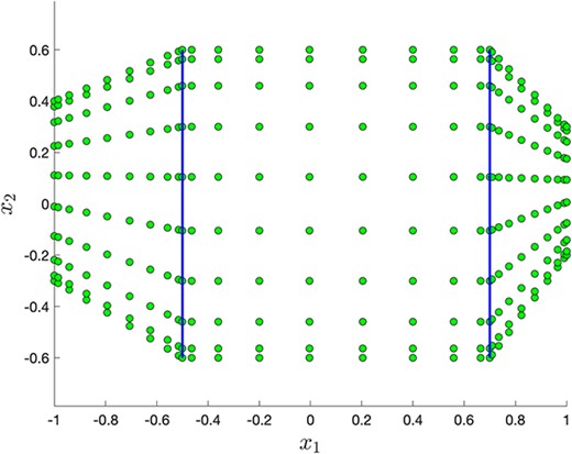
Constructing the normal vectors on the boundary of the multishape is necessary to compute no-flux boundary conditions and inter-element matching conditions. The starting point is again to consider the normals for each individual element, and in particular those lying on the boundary of the multishape. However, at the intersection corners between two elements, these normal vectors are not defined consistently. In this case the code considers the normal vectors on the multishape boundary to both sides of the intersection corner and averages them. In order to do this correctly, all normals first have to be converted into Cartesian coordinates, averaged and converted back into polar coordinates where appropriate. For more complicated multishape domains, taking the average of adjacent normals may not be sufficient, and the resulting outward normal may not be sensible. Since this can be very specific to the discretization at hand, the option to plot and, if necessary, override any of the normal vectors manually is given. Such a case is demonstrated in Fig. 2.
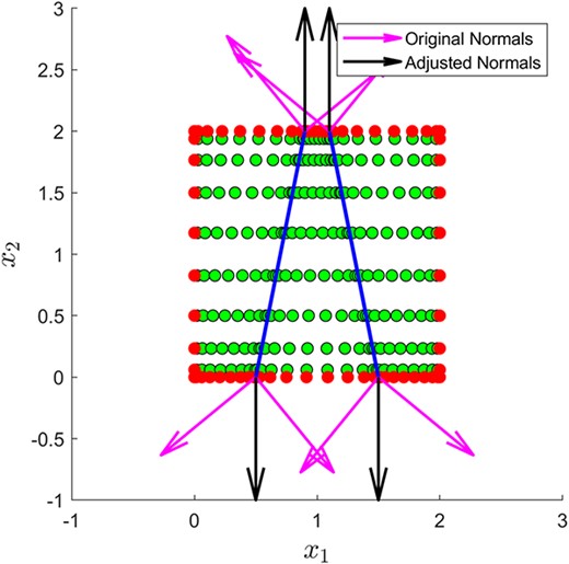
Overriding the normal vectors at intersection corners, which are automatically constructed by MultiShape, to ensure they are defined in the normal direction to the multishape face on which the intersection corner is located.
2.2.6 Integration and convolution
The computation of convolution integrals is the final part of the MultiShape implementation that we discuss here. Since computing a convolution integral is a global operation, we cannot rely on reusing the computations on individual elements. However, the general steps are equivalent to the approach for a single element and it is therefore recommended to refer to Nold et al. (2017) for details. A brief outline of constructing the convolution matrix is given below. A convolution integral is defined as
for a density |$u$| and a weight function, or kernel, |$\chi $|. Integration on the multishape is defined element-wise, using Clenshaw–Curtis quadrature Clenshaw & Curtis (1960), as discussed in Section 2.2. Denoting the integration vector by Int and defining |$ \vec y - \vec z: = \vec x$|, the convolution matrix can be computed by
where the subscripts |$1$| and |$2$| refer to the two dimensions of the domain, while |$m, n \in \{1,...,M\}$| denote matrix (vector) entries, with |$M$| the total number of points in the multishape. In particular, |$\text{Int}_{n}$| is the |$n$|th element of the |$1 \times M$| integration vector. If the function |$\chi $| only takes one input, we consider
where |$\| \cdot \|_{2}$| denotes the standard Euclidean distance. The convolution integral is now defined as a matrix–vector multiplication, by applying the matrix Conv to a density vector |$u$|. This is contrasted by the FFT approach for solving convolution integrals Roth (2010). Therein, at each iteration a Fourier transform of |$u$| is taken, and the convolution theorem is applied to yield
Since the FFT approach relies on periodicity of the domain, it is not easily applied to the complicated multishape domains considered in the present work. The present approach is also amenable to applying complicated nonperiodic boundary conditions, which is highly challenging using the FFT approach. Moreover, it can lead to significant computational advantages within iterative algorithms, including ODE solvers and optimization routines, since the convolution matrix does not have to be recomputed at each iteration with changing |$u$|. A discussion of the advantages and drawbacks of the two methods applied to simple domains can be found in Nold et al. (2017). We note that, although the approach taken here formally does not scale as well as an FFT approach (roughly |$N^{2}$| vs. |$N\ln (N)$| for |$N$| total points), this comparison is not entirely meaningful. First, as is generally the case with pseudospectral methods, |$N$| is not typically (asymptotically) large. Secondly, the application of such FFT methods to complicated domains, or to cases where the kernel of the convolution has bounded support, is highly nontrivial, and likely needs a bespoke implementation for different kernels and domains. In contrast, the approach here is general and modular.
2.3 PDE discretization and solution
Using MultiShape to discretize a PDE and apply boundary and intersection conditions is straightforward. By dividing |$\varOmega $| into |$n_{e}$| sub-elements forming a multishape, a discretized version of problem (2.1) for the unknown |$\mathbf u$| defined on each sub-element, is given by
where the mass matrix |$M_{\varOmega }$| for a collocation method is diagonal, and |$\mathbf{f}$| is the discretization of the right-hand side of the PDE. The patching method’s matching conditions, introduced in Section 2.1.1, and boundary conditions (imposed by |$\varGamma $|) are applied by setting the relevant (diagonal) entries in the mass matrix to zero and suitably adapting the right-hand side of the discretized PDE. Differentiation and convolution matrices relevant to the PDE discretization are constructed automatically by the MultiShape library and are applied to the vector |$\mathbf u$| on the right-hand side of (2.6) by using matrix–vector multiplication. The matching conditions are applied via an inbuilt function, which uses the intersection boundaries that are identified during construction of the multishape. Similarly, the code automatically identifies the boundary of the multishape, so that the boundary conditions of the PDE can be applied in the same way as for single shapes in 2DChebClass. MultiShape constructs the vector |$\mathbf{f}$| (with entries dependent on the PDE that the user has supplied), automatically sets the mass matrix entries in |$M_{\varOmega }$| and, lastly, appropriately modifies the entries of |$\mathbf{f}$| corresponding to matching or boundary conditions.
In turn, MultiShape transforms the boundary value problem (2.1) into a discrete system of ODEs (2.6). For the time integration, MultiShape implements the Matlab DAE solver ode15s, which has been optimized to give good performance for a wide range of stiff ODEs. However, in some instances, problem-specific computational speed-ups may be exploited by alternative time integrators. MultiShape allows users to implement their own schemes in this case.
In this subsection we provide a concrete instance of the MultiShape computation described above, along with listings displaying the typical user interface, applied to an example in DDFT. This example illustrates the power of MultiShape to solve physically-motivated, complex, nonlinear PDEs with nontrivial boundary conditions, with the user freed from laborious preparation associated with the geometrical details of the PDE to be solved. We demonstrate how a multishape is set up by the user, and describe the information that needs to be provided in order to solve a PDE problem on the multishape using the DAE solver ode15s in Matlab.
2.3.1 Making a multishape
In order to set up a multishape, each element has to be defined, as well as an order in which they are arranged, from |$1$| to |$n_{e}$|, although this ordering is essentially arbitrary. For each element the number of discretization points, |$N_{1}$| in the |$x_{1}$|-direction, |$N_{2}$| in the |$x_{2}$|-direction, needs to be specified. To uniquely determine a shape, for a quadrilateral element it suffices to specify the corners; a wedge element is defined in polar coordinates, by specifying an inner and outer radius, a minimum and maximum angle, and the location of the origin.
2.3.2 Inter-element conditions
Matching conditions are applied at the intersections between two elements |$e_{i}$| and |$e_{j}$|. However, other conditions can be applied at the intersection boundary between two elements. For example, the MultiShape library additionally supports the application of no-flux boundary conditions between elements, modelling a hard wall, and the inclusion of other matching options into the code library is straightforward. Which condition to apply on each intersection between elements |$e_{i}$| and |$e_{j}$|, is specified simply by setting a flag. The code demonstrating how to set up a multishape, and provide the necessary geometrical and numerical information, is found in Listing 1. The resulting multishape (with different numbers of points) can be seen in Fig. 1. Note that, in order to create a functioning multishape, the number of points of the neighbouring faces of two elements have to match, as discussed in Section 2.2. Once the multishape is set up, and necessary user-defined quantities are provided (see Listing 2), required operators and properties, such as differentiation matrices or the location of boundary points, can be simply extracted from the multishape structure, as demonstrated in Listing 3.
2.3.3 Solving a PDE in MultiShape
A fully functional example MultiShape source file, including shape, PDE, boundary and matching definitions, is illustrated in Listing 1–5. It can be run within a function environment in Matlab. The example problem is PDE problem (2.1) of gradient flow type, as introduced in Section 2.1, with the flux given by (2.2). Note that the codes in Listings 3–5 are independent of the specific multishape that is defined in Listing 1. If one were to compute the same PDE system on a different multishape, the only part of the code that needed to be amended would be in Listing 1, demonstrating the modularity of the code. Similarly, only the input in Listing 2 needs to be modified in order to change the initial condition |$u_{0}$|, the time horizon of the problem, or user defined potentials |$V_{\text{ext}}$| and |$V_{2}$| (so that |$\vec w:= \nabla V_{\text{ext}}$| and |$\vec K:= \nabla V_{2}$| in (2.2)). Note that several ‘helper functions’ are defined within MultiShape, which support straightforward implementation. These include masks to access individual elements of the multishape, computation of inner products between two vectors and the application of intersection boundary conditions, as discussed in Section 2.2. Discretizing the right-hand side of the PDE, |$\mathbf{f}(\mathbf u(t),t)$|, is illustrated in Listing 4. Note that the nonlocal no-flux boundary conditions (4.4) are applied in Listing 4 in a single line of code (line 18), demonstrating the ease of implementation of complicated boundary conditions.
Setting up a multishape.
 |
|
Setting up a multishape.
|
|
Additional user defined input for solving a PDE problem.
 |
|
Additional user defined input for solving a PDE problem.
|
|
Extracting operators. [Input from Listing 2: V2. Inbuilt function: MS.ComputeConvolutionMatrix.]
 |
|
Extracting operators. [Input from Listing 2: V2. Inbuilt function: MS.ComputeConvolutionMatrix.]
|
|
Discretizing the right-hand side of the PDE system. [Input from Listing 2: Vext. Operators from Listing 3: |$ \texttt{grad}, \texttt{div}, \texttt{bound}, \texttt{normal}.\ Inbuilt\ functions{:} \\ \texttt{MS1.ApplyIntersectionBCs}, \texttt{MS.MakeVector} $|.]
 |
|
Discretizing the right-hand side of the PDE system. [Input from Listing 2: Vext. Operators from Listing 3: |$ \texttt{grad}, \texttt{div}, \texttt{bound}, \texttt{normal}.\ Inbuilt\ functions{:} \\ \texttt{MS1.ApplyIntersectionBCs}, \texttt{MS.MakeVector} $|.]
|
|
Solving a PDE system on a multishape using Matlab's DAE solver. [Inputs from Listing 2: |$\texttt{comp_times}, \texttt{u_ic} $|. Operators from Listing 3: |$\texttt{bound}, \texttt{intersections} $|.]
 |
|
Solving a PDE system on a multishape using Matlab's DAE solver. [Inputs from Listing 2: |$\texttt{comp_times}, \texttt{u_ic} $|. Operators from Listing 3: |$\texttt{bound}, \texttt{intersections} $|.]
|
|
3. Validation of MultiShape methodology
This section contains validation tests for our MultiShape implementation, investigating the accuracy of the differentiation, integration, interpolation and convolution operations. We further validate our methodology by computing the solution to a Poisson problem with Dirichlet boundary. All of these tests have been carried out by comparing the numerical results to analytic solutions. In all tests exponential convergence is observed, until a certain threshold is reached, which is mostly dictated by machine precision, and to a lesser extent by compounding precision or interpolation errors. Additionally, to demonstrate the flexibility of our methodology, we compare the optimize-then-discretize and discretize-then-optimize approaches for a Poisson control problem, and tackle a wave equation using LGL collocation points.
Most errors in this section are calculated using a relative numerical |$L^{2}$| norm defined as
where |$f_{\text{Num}} $| and |$f_{\text{Ex}}$| correspond to numerical and exact solutions, and the additional (arbitrary) small term in the denominator is added to avoid the possibility of division by zero—the results do not change significantly for other reasonable values. The interpolation error is calculated in the same way, but replacing the |$L^{2}$| norm by a (vector) |$\ell ^{\infty }$| norm. This is because the error is calculated on a uniform grid and not a Chebyshev grid, so that computation of the |$L^{2}$| norm would require numerical integration in uniform space, which would introduce larger integration errors than the Clenshaw–Curtis integration formula Clenshaw & Curtis (1960) implemented in MultiShape. Since integration results in a single number, for such computations, the |$L^{2}$| norm in (3.1) is replaced by taking absolute values, with |$f_{\text{Num}}$| and |$f_{\text{Ex}}$| the numerical and exact integrals, respectively.
3.1 Validation of discretized operators
The multishapes considered in this validation section are discretizations of boxes and wedges. This is so that comparisons can be made with the 2DChebClass implementation for a single shape. The different discretizations considered for a variety of test cases can be seen in Figs 3 and 4. The four discretizations of a box in Fig. 3 include a reference multishape, discretizations with varying number of elements, uneven splits of the domain, as well as a discretization that contains an interior point, at which four elements intersect, (d). The wedge discretizations in Fig. 4 include a reference multishape, a multishape that is discretized in the radial direction as well as one in the angular direction and a discretization containing three elements. The total number of points |$N_{\varSigma }$| in each direction for the discretizations in Figs 3 and 4 varies, and those chosen for the plots are for illustration purposes only. For example, in discretization (d) we take |$N_{\varSigma } = 14$|, which results in |$7$| points in each direction for each of the four elements.
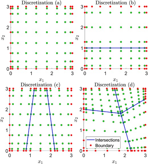
Different multishape discretizations of a box (a–d).
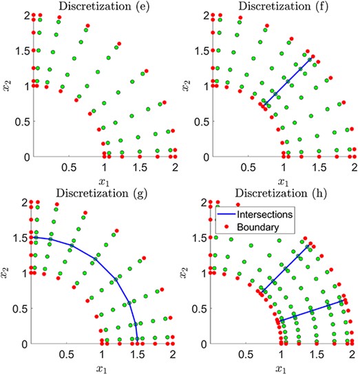
Different multishape discretizations of a wedge (e–h).
The three differentiation operators, that is, gradient, divergence and Laplacian, are validated by comparing against an exact solution. The test function considered is
which is also used to test the accuracy of the interpolation matrix. This is tested by interpolating |$g_{1}(x_{1},x_{2})$| onto a (uniform) target grid defined by |$x_{1,U}$|, |$x_{2,U}$| and comparing the result to |$g_{1}$| evaluated directly on the target grid. The choice of |$g_{1}$| is largely arbitrary; similar results were obtained for a wide range of functions. This is also the case with the functions chosen below for other validation tests. For integration we choose the (Gaussian) test function
To test the convolution operator we have two different pairs of test functions
where |$\chi _{C}$|, |$n_{C}$| are considered for Cartesian discretizations and |$\chi _{P}$|, |$n_{P}$| are the test functions on polar multishapes. This is to facilitate the analytical computation of the convolutions.
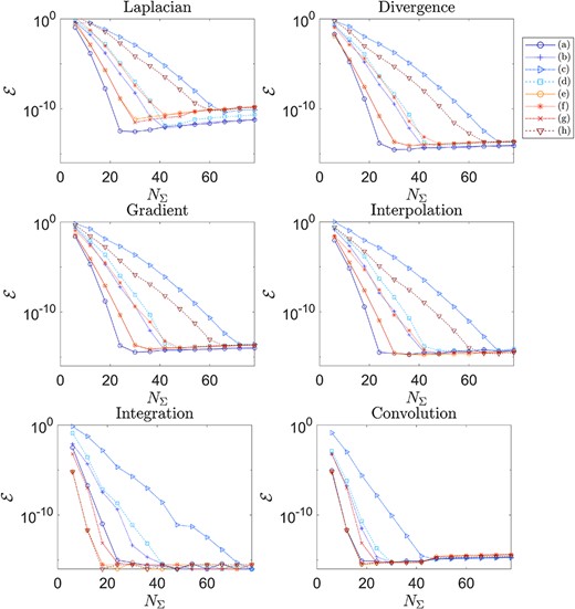
The error, as defined by (3.1), in the numerical differentiation, integration, interpolation and convolution operators. Errors are computed for varying numbers of discretization points |$N_{\varSigma }$| and measured against an exact solution.
The convergence resulting from computations with the Laplacian, divergence, gradient and interpolation matrices on different discretizations can be seen in Fig. 5. As expected, convergence to the exact solution is observed as the number of discretization points is increased. For each discretization, the total number of points in each of the |$x_{1}$| and |$x_{2}$| directions (over the whole multishape), denoted by |$N_{\varSigma }$|, remains the same. Since the overall number of points for each multishape is the same, the computational cost for each discretization is fixed and so the performance of each discretization choice can be compared. For each multishape, the |$N_{\varSigma }$| points are equally distributed among the different elements. However, as the following comparison demonstrates, a minimum number of points has to be allocated in each the |$x_{1}$| and |$x_{2}$| directions and on each element of the multishape, in order to achieve optimal convergence. Multishape (c) in Fig. 3 is discretized into three elements in such a way that the number of points in the |$x_{1}$| coordinate is split three ways, resulting in each element only having |$N_{\varSigma }/3$| points in the |$x_{1}$| coordinate, and subsequently a poorer overall convergence than, for example, in multishape (d). While multishape (d) is discretized into four shapes, the |$x_{1}$| and |$x_{2}$| coordinate are only divided once, so that each element has |$N_{\varSigma }/2$| points in each direction, improving convergence considerably.
3.2 Method of manufactured solutions: the Poisson equation
Having validated the convergence of different operators on different multishapes, for the next test we solve a Poisson problem. This demonstrates that applying the intersection matching conditions between the elements of a multishape works as expected, without adding further complexities, such as PDE solvers or integral terms. We solve the Poisson equation
The right-hand side of the PDE,
is chosen such that the Poisson equation on an infinite domain
has an exact solution, |$v(\vec x) = \exp (-0.5((x_{1}-0.5)^{2} +(x_{2}-0.5)^{2}))$|. This can then be used to test the accuracy for the numerical solution to the Poisson problem (3.2), by enforcing the nonconstant Dirichlet boundary conditions |$u(\vec x) = v(\vec x)$| on the multishape boundary. As in Section 3.1, we test the convergence on the different discretizations of the box (Fig. 3) and wedge (Fig. 4), for a varying number of discretization points, as displayed in Fig. 6.
![The error, as defined by (3.1), in computing the solution to the Poisson equation on different discretizations of a box and a wedge. Errors are computed for varying numbers of discretization points $N_{\varSigma }$ and measured against an exact solution. [Note that for (c), with $N_{\varSigma } = 6$ no interior points in $x_{1}$ are present, so this data point is omitted.]](https://oup.silverchair-cdn.com/oup/backfile/Content_public/Journal/imajna/PAP/10.1093_imanum_drae066/2/m_drae066f6.jpeg?Expires=1750600573&Signature=hXwMd9HBaU2OdNeMCDp5gfyl~33olInGMefIIp3ta7ykdwJhmqjlkpOJoFowCeMBCYykZyfq7CcZy5VvbGAnILkoDCN1TGJemt~4b5Z2AX53kl45~XL6wg1-YySwGxPzrb9HYNZIBUhfl6mmPMchZChWlh3ZBSCriuDcGz7IGOfLfZ3RqSDS9-MKrdKx95v3UeJRVZGvJuO-GGfMqM8YKC71BWIfOQ3SUuAIzOptZLmAgqKfqwRjwej2SX6YukEundg8KpQYxncTsDrLuRbOhDwh4sG~cDCZPzr3lhKb2GpnzK5RMhQfoJEuN4TWclS6wrKbpmHG3JKKz3DUoqpnQg__&Key-Pair-Id=APKAIE5G5CRDK6RD3PGA)
The error, as defined by (3.1), in computing the solution to the Poisson equation on different discretizations of a box and a wedge. Errors are computed for varying numbers of discretization points |$N_{\varSigma }$| and measured against an exact solution. [Note that for (c), with |$N_{\varSigma } = 6$| no interior points in |$x_{1}$| are present, so this data point is omitted.]
Similarly, the solution to the Poisson equation on a multishape, which combines a quadrilateral and a wedge element, as in Fig. 1, is computed. Intersection matching conditions are applied between the two elements as illustrated in Section 2.2. Note that the two elements are not defined in the same coordinate system, which MultiShape automatically takes into account when applying the intersection condition. The three test cases considered involve taking equal numbers of points in both coordinate directions, half the number of points in the first coordinate direction (|$x_{1}$| and |$r$|, respectively), and half the number of points in the second coordinate direction (|$x_{2}$| and |$\theta $|, respectively). We compare the error in the numerical solution to the Poisson problem (3.2) with the resulting computational timings. Figure 7 showcases the convergence of the numerical result to the exact solution with increasing time, which correlates with increasing total numbers of discretization points. The results in Fig. 7 demonstrate that the distribution of points among the coordinate directions does not result in a large difference in computation time taken for comparable accuracy in the resulting solution. However, the most efficient discretization for the particular choice of multishape and Poisson problem appears to be distributing double the points in the |$x_{2}$| and angular directions than in the |$x_{1}$| and radial directions.
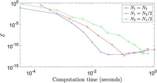
The error, defined by (3.1), in solving the Poisson equation on a multishape, against computation time, for varying numbers of discretization points in the two coordinate directions, |$N_{1}$| and |$N_{2}$|, for each element.
3.3 Optimization problem involving the Poisson equation
As a further demonstration of the power of the MultiShape approach, we now apply it to optimal control problems involving PDEs. Here, we consider the Poisson control problem
subject to the PDE constraint
Here, |$u$| and |$w$| are referred to as state and control variables, with |$\widehat{u}$| a given desired state, and |$\beta>0$| is a regularization parameter. We compare the optimize-then-discretize (OTD) and discretize-then-optimize (DTO) approaches for solving such a PDE-constrained optimization problem. The OTD approach involves deriving adjoint and gradient equations through Fréchet differentiation with respect to |$u$| and |$w$|, alongside the state equation (3.3), on the continuous level, then discretizing these constraints (see (Tröltzsch, 2010, Chapter 2)). Conversely, the DTO approach involves first deriving a discrete analogue of the above control problem, and then obtaining optimality conditions through differentiation on the discrete level. Note that we restrict ourselves to a local problem here, and we tackle an optimization problem with a nonlocal PDE constraint in Section 4.2. Our aim here is to demonstrate that the OTD and DTO approaches can both be tackled within the MultiShape formalism.
For this illustration, we choose the domain shown in Fig. 8 (using 14 points in each direction for each shape; note that this varies in the following calculations). We set the desired state |$\widehat{u}(\vec x) = 1 - \text{cos}(\pi x_{1})$|, with |$g(\vec x) = \widehat{u}(\vec x)$| on |$\partial \varOmega $|. In Table 1 we provide the values of the cost functionals and their relative difference, approximated by pseudospectral quadrature, for a range of numbers of discretization points |$N$| (for simplicity, fixed to be the same in each direction and for each shape), and regularization parameters |$\beta $|.
Domain for comparison of the OTD and DTO approaches for the Poisson control problem.
Comparison of the cost functionals for the OTD and DTO approaches for solving the Poisson control problem described in Section 3.3. Here, for different choices of the number of collocation points (|$N$|) and regularization parameter (|$\beta $|), |$\mathcal{J}_{\mathrm{OTD}}$| and |$\mathcal{J}_{\mathrm{DTO}}$| denote the cost functional for the OTD and DTO approaches, respectively; |$\mathcal{J}_{\mathrm{diff}}$| denotes the relative difference |$|\mathcal{J}_{\mathrm{OTD}} - \mathcal{J}_{\mathrm{DTO}}|/|\mathcal{J}_{\mathrm{OTD}}|$|
| |$N$| | |$\beta $| | |$1$| | |$10^{-1}$| | |$10^{-2}$| | |$10^{-3}$| | |$10^{-4}$| |
|---|---|---|---|---|---|---|
| |$\mathcal{J}_{\mathrm{OTD}}$| | 1.37e-1 | 1.27e-1 | 7.69e-2 | 2.21e-2 | 3.59e-3 | |
| 10 | |$\mathcal{J}_{\mathrm{DTO}}$| | 1.37e-1 | 1.26e-1 | 7.68e-2 | 2.20e-2 | 3.57e-3 |
| |$\mathcal{J}_{\mathrm{diff}}$| | 5.97e-5 | 5.17e-4 | 1.70e-3 | 1.49e-3 | 5.71e-3 | |
| |$\mathcal{J}_{\mathrm{OTD}}$| | 1.37e-1 | 1.27e-1 | 7.69e-2 | 2.21e-2 | 3.59e-3 | |
| 15 | |$\mathcal{J}_{\mathrm{DTO}}$| | 1.37e-1 | 1.27e-1 | 7.69e-2 | 2.21e-2 | 3.58e-3 |
| |$\mathcal{J}_{\mathrm{diff}}$| | 3.10e-5 | 2.68e-4 | 8.56e-4 | 6.44e-4 | 2.79e-3 | |
| |$\mathcal{J}_{\mathrm{OTD}}$| | 1.37e-1 | 1.27e-1 | 7.69e-2 | 2.21e-2 | 3.59e-3 | |
| 20 | |$\mathcal{J}_{\mathrm{DTO}}$| | 1.37e-1 | 1.27e-1 | 7.69e-2 | 2.21e-2 | 3.58e-3 |
| |$\mathcal{J}_{\mathrm{diff}}$| | 1.59e-5 | 1.38e-4 | 4.56e-4 | 4.05e-4 | 1.61e-3 | |
| |$\mathcal{J}_{\mathrm{OTD}}$| | 1.37e-1 | 1.27e-1 | 7.69e-2 | 2.21e-2 | 3.59e-3 | |
| 25 | |$\mathcal{J}_{\mathrm{DTO}}$| | 1.37e-1 | 1.27e-1 | 7.69e-2 | 2.21e-2 | 3.58e-3 |
| |$\mathcal{J}_{\mathrm{diff}}$| | 1.16e-5 | 1.00e-4 | 3.22e-4 | 2.46e-4 | 1.08e-3 | |
| |$\mathcal{J}_{\mathrm{OTD}}$| | 1.37e-1 | 1.27e-1 | 7.69e-2 | 2.21e-2 | 3.59e-3 | |
| 30 | |$\mathcal{J}_{\mathrm{DTO}}$| | 1.37e-1 | 1.27e-1 | 7.69e-2 | 2.21e-2 | 3.59e-3 |
| |$\mathcal{J}_{\mathrm{diff}}$| | 7.42e-6 | 6.43e-5 | 2.13e-4 | 1.89e-4 | 7.55e-4 |
The results indicate that the computed cost functionals converge to a fixed value as |$N$| increases for each |$\beta $|, as expected, and that this value gets smaller as |$\beta $| decreases. We observed that the approximated values of |$\mathcal{J}_{\mathrm{DTO}}$| were slightly lower than those of |$\mathcal{J}_{\mathrm{OTD}}$|, but the relative differences between the computed cost functionals using the OTD and DTO approaches are very small. The relative differences between these values decrease as |$N$| increases, indicating the viability of each strategy within the MultiShape framework.
3.4 LGL collocation points and the wave equation
Whilst Chebyshev collocation points are often regarded as the best choice for nonperiodic domains (Boyd, 2001, Section 1.6), there are many other reasonable choices of pseudospectral discretizations. One of the key benefits of the MultiShape architecture is that, in order to introduce new collocation schemes, one only needs to provide the one-dimensional points, integration weights and differentiation matrices. The bulk of the code is agnostic to these choices and can be easily re-used in a modular fashion. To demonstrate this flexibility, we also provide support for the LGL collocation points.
In contrast to the Chebyshev discretization (2.5), there is no closed form for the LGL collocation points. Rather, they are given by (Canuto et al., 2006, Section 2.3)
where |$L_{N}$| is the |$N$|th Legendre polynomial and here the prime denotes differentiation. The integration weights and differentiation matrices have closed forms, but they involve evaluating Legendre polynomials at the (numerical approximations of the) |$x_{j}$| (Canuto et al., 2006, Sections 2.3–2.4); note that there is a missing factor of 2 in the expression of the second-order differentiation matrix given in (Canuto et al., 2006, Eq. (2.4.36)). Here, we choose to determine the |$x_{j}$| by a Newton–Raphson method, which evaluates them to floating point accuracy.
In order to demonstrate the use of this discretization, and also the solution to a second-order-in-time PDE, we solve the wave equation
Here the enforced boundary condition is purely for convenience; it is also straightforward to impose a no-flux boundary condition, for example. The challenge is then to determine a nontrivial initial condition that is consistent with the boundary conditions on a complicated domain.
For the example here, we choose a multishape consisting of four quadrilaterals, resulting in a ring-like structure with outer corners at |$(3,-3)$|, |$(-2.5,1.7)$|, |$(2,1.5)$|, |$(4,-3.5)$|, and inner corners at |$(-1,-1)$|, |$(-1.1, 0.6)$|, |$(1.2,0.5)$|, |$(1,-0.8)$|. Note that these choices are essentially arbitrary. For the results in Fig. 9, we use 16 points in each direction for each shape; increasing this does not change the solution appreciably. The computation takes approximately 1 minute.
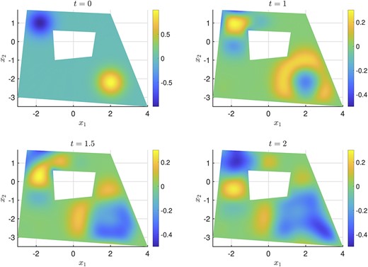
Solution of the wave equation (3.4) using the LGL discretization.
For the initial condition we choose, with considerable flexibility available to us here,
with |$x_{1,a} = 2$|, |$x_{2,a} = -2.2$|, |$x_{1,b} = -1.8$|, |$x_{2,b} = 1$| and |$\alpha = 2$|.
In Fig. 9, we present snapshots of the solution at various times. Note that these are visually indistinguishable from the solution to the same problem computed using the Chebyshev discretization. As is standard, the second-order (in time) PDE is solved by writing it as a system of two first-order equations:
with appropriate initial and boundary conditions. For the MultiShape implementation, we note that no matching conditions on the intersections are required for |$u$| (since it is local in space), whilst for |$v$| we employ the standard matching conditions (2.3) and (2.4).
4. Applications to physically-motivated problems
An important motivation for developing this MultiShape methodology is its ability to solve nonlocal, nonlinear PDEs on unusual physical domains. Often, real world problems are posed on geometries more complicated than rectangles or discs, as is common in, e.g., fluid flows in and around pumps and vanes in industrial settings, in brewing vessels, or microfluidic flows in biological sciences. In the following subsections, we will introduce the necessary background and relevant models, as well as numerical solutions obtained by a MultiShape implementation, for a single example in two classes of problems increasingly used in the modelling of industrial processes: DDFT and control problems. DDFT models involve the added complexity of nonlinear, nonlocal terms, which are challenging to tackle using standard methods, such as FEMs, as discussed in the Introduction. This becomes even more expensive when combined with optimization problems. We show that MultiShape may be applied to efficiently solve such problems on complicated domains. Throughout this section, problems involving the models are solved numerically on a multishape, with appropriate intersection conditions applied between multishape elements. All tests are carried out on Dell PowerEdge R430 running Scientific Linux 7, four Intel Xeon E5-2680 v3 2.5GHz, 30M Cache, 9.6 GT/s QPI 192 GB RAM and using Matlab Version 2021b.
4.1 A DDFT model
The DDFT describes how a one-body particle density |$\rho $| changes depending on time and the free energy of the system |$\mathcal F$|. This results in, often complicated, integro-PDE models. An extensive overview of the various applications of the theory is provided in te Vrugt et al. (2020). In this work we focus on a DDFT model that includes particle interactions via a mean-field model, and leave more complex formulations that describe effects such as (hard-core) volume exclusion for future study. This idea is easily extended to a system with more than one particle species. The |$n_{s}$| integro-PDEs that describe the dynamics of a system with |$n_{s}$| species of particles, with densities |$\rho _{a}$|, for |$a = 1,...,n_{s}$|, are of gradient flow form
where |$\mathcal{F}$| is the Helmholtz free energy functional depending on all species |$b = 1,..,n_{s}$|.2 The free energy of a system is composed of an ideal gas contribution, as well as contributions from an external potential and from particle–particle interactions. Under the mean-field approximation, such a system has a free energy functional given by
where |$V_{\text{ext}}$| is an external potential and |$V_{a,b}$| are potentials, describing the interactions between species |$a$| and |$b$|. Note that here the de Broglie wavelength |$\varLambda = 1$|, and |$k_{B}T = 1$|. In this work, the interaction potential is given by
where |$\sigma _{a,b}$| represents half of the distance between the centres of particle |$a$| and particle |$b$| and with interaction strength |$\kappa _{a,b}$|. If |$a = b$|, this can be thought of as the particle radius. Again, the results of the method are highly robust under different choices of |$V_{a.b}$| (not shown here). After inserting the free energy into (4.1), we obtain a system of PDEs of the form
with appropriate initial and boundary conditions. We focus here on no-flux boundary conditions, since they are some of the most complicated conditions to apply, in particular for nonlocal problems, and are highly relevant for applications. These are defined as
on |$\partial \varOmega $|, where |$\vec n$| is the outward normal and |$\frac{\partial }{\partial n}:=\vec n \cdot \nabla $| denotes the partial derivative with respect to this normal. We restrict our numerical example to particle dynamics of two species; however, extension to higher numbers of species is straightforward. Note that this problem is of the form (2.1), when setting |$u = [\{\rho _{a}\}]$| and |$f= [\{f_{a}\}]$|, for |$a,b= 1,2,...,n_{s}$|.
4.1.1 Equilibrium solutions
There are two equivalent approaches to finding steady states of (4.1); investigating the behaviour of (4.1) for large |$t$|, such that |$\frac{\partial \rho _{a}}{\partial t} \approx 0$|, or minimizing |$\mathcal F$| with respect to |$\rho _{a}$|. Focusing on the latter approach, the Euler–Lagrange equation for minimizers |$\rho _{a}$| is |$\frac{\delta{\mathcal F}}{\delta \rho _{a}} = 0$|. It may be shown that |$\rho _{a}$| is a minimizer if and only if it is a fixed point of the self-consistency equation
where |$Z^{-1}$| is a normalization constant, enforcing that the mass of, and therefore the number of particles in, the system is fixed. Note that problems in equilibrium Density Functional Theory (DFT) also require finding a minimum of a free energy |$\mathcal F$|, and can therefore be tackled by such variational approaches. Overviews of DFT are given in, e.g., Evans (1979); Löwen (1994); Wu (2006); Wu & Li (2007). The system of equations (4.5) is of the form |$\rho _{a} = G_{a}(\rho _{1},...,\rho _{n_{s}})$| and can be solved using, for example, iterative methods. As above, in this work, we are considering a system of two species, which demonstrates all relevant features of the numerical solution, but this can easily be extended to systems with more species. In order to find the solution to the self-consistent system of equations (4.5), we use an iterative scheme, known as Picard iteration in the DDFT community Roth (2010), which is described in Appendix A. Note that this is a damped version of a standard fixed-point iterative scheme, which is widely used in numerical analysis.
For this example, we consider two species, with |$n_{s} = 2$|. A multishape is defined using three elements: two quadrilaterals and one wedge; see Fig. 10. The number of points in each shape is |$N_{1} = N_{2} = 30$|. The interaction strengths, for an interaction potential of the form (4.2), were chosen as |$\kappa _{1,1} = -7$|, |$\kappa _{2,2} = -3$|, |$\kappa _{1,2} = \kappa _{2,1} = 2$|, with |$\sigma _{1,1} = 0.1$|, |$\sigma _{2,2} = 1$|, |$\sigma _{1,2} = \sigma _{2,1} = 0.55$|. This simulates Species |$1$| being significantly smaller than Species |$2$|, with intra-species attractive potentials and inter-species repulsion. We furthermore impose an external potential |$V_{\text{ext}} = 0.1x_{2}$|, simulating gravitational forces acting on the particles. While the equilibrium results are robust for different choices of initial guesses, we choose |$\rho _{1,\text{ic}}$|, |$\rho _{2,\text{ic}}$| of the form
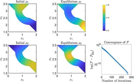
Equilibrium solution for a two-species system on a multishape. Bottom right: convergence of the free energy |$\mathcal F$|, measuring the log change in |$\mathcal F$| shifted by the final value of the free energy |$\mathcal F_{\text{fin}}$| in order to compare the differences in free energy rather than absolute values.
with |$c_{M} = 1$| and density functions of the form
which will be seen as valid choice, compatible both with the self consistency equation (4.5) and the no-flux condition on the boundary (4.4), since they are relatively far from both the equilibrium and each other.
With this choice of initial guesses, a mixing parameter choice of |$\lambda = 0.5$| and a termination tolerance of |$10^{-8}$|, Algorithm A.1 converges to an equilibrium state within |$266$| iterations, taking |$24$| seconds. The initial conditions, the equilibrium solution, as well as the convergence of the free energy of the system, are displayed in Fig. 10. We choose to display the convergence of the free energy instead of, say, the difference between two successive iterates of |$\rho $|, as this is a physical quantity of importance to practitioners. In the equilibrium solution, the interplay between the gravitational forces and particle interactions can be observed. Since Species |$1$| and |$2$| repel each other, they are found to separate within the domain. Furthermore, we see that since Species |$1$| is smaller in size than Species |$2$|, it clusters at the boundary of the domain, while Species |$2$| accumulates in the middle, which agrees with physical intuition. One can use the same initial guesses as initial conditions for the time-dependent equation (4.3), with time horizon |$(0,50)$| and DAE solver tolerances set to |$10^{-9}$|, the solution of which takes |$7$| minutes. The error (3.1) between the equilibrium computation and the long term solution of the dynamic problem is |$2.6424 \times 10^{-5}$|, which is a good indication that the solution to (4.5) obtained by the Picard Algorithm A.1 corresponds to an asymptotically stable equilibrium state of the dynamics (4.3), while being computationally advantageous.
For completeness, in Fig. 11, we display the convergence of the solutions for the two species as we increase |$N_{1} = N_{2} = N$|, where we display the |$L^{2}$| relative error between the final solutions of the Picard algorithm and that computed with |$N=40$| points, which we take as a reference, ‘exact’ solution. We note that, for |$N=30$|, the error is comparable to the termination tolerance of the Picard iteration.
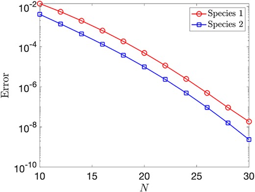
Convergence of the Picard scheme as |$N_{1} = N_{2} = N$| increases. Note that here ‘Error’ denotes the |$L^{2}$| relative error between the solution and that computed with |$N=40$| points, which we take as a reference, ‘exact’ solution.
4.1.2 Time-dependent solutions
We now consider an example of the dynamic model introduced in Section 4.1, which models a funnel through which particles of different sizes are passing. Once again, there are two types of particles in the system, one species being larger than the other. We expect that smaller particles should pass through the narrow part of the funnel more easily than the larger particles. We introduce an external potential |$V_{g} = c_{g} x_{2}$|, modelling gravity, with |$c_{g} = 0.15$|. To illustrate the ability of MultiShape to handle nontrivial boundary effects, the left and right walls of the funnel are repulsive. This is a simple way to approximate volume exclusion effects. Since the two species are of different sizes, the repulsion is of different strengths. The external potential, modelling the repulsive walls, is defined as
where |$d_{L}$| and |$d_{R}$| are the shortest (Euclidean) distances from the point |$\vec x$| to the left and right boundary of the multishape, respectively. We choose |$\epsilon = 0.6$|, |$\alpha _{1} = 0.5$| for Species |$1$| and |$\alpha _{2} = 2$| for Species |$2$|. The interactions between particles are again described by the potential (4.2), but this time with the choice |$\kappa _{1,1} = \kappa _{2,2} =\kappa _{1,2} = \kappa _{2,1} = 0.1$| and corresponding |$\sigma _{1,1} = 0.5$|, |$\sigma _{2,2} =2$|, |$\sigma _{1,2} = \sigma _{2,1} = 1.25$|. The choice of |$\sigma _{2,2}$| is motivated by the fact that the narrow channel in the multishape has width |$2$|. The initial conditions for each species are similarly of the form (4.6), with |$f_{1,\text{ic}} = f_{2,\text{ic}} = x_{1} + 5$| and |$c_{M} = 20$|. The time interval for this simulation is |$t \in [0,20]$|, and each element in the multishape is discretized using |$N_{1} = N_{2} = 20$| points. The DAE solver ode15s, with absolute and relative tolerances set to |$10^{-9}$|, takes around |$20$| seconds to solve this problem and the result is displayed in Fig. 12.
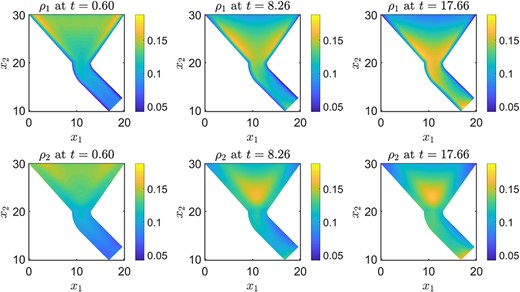
Dynamics of two interacting species of different size in a funnel under the influence of gravitational forces.
It is evident that the behaviour of the two species is qualitatively different. Due to their size, the larger particles gather in the middle of the funnel, while the smaller particles gather at the boundaries. Both species experience the repulsion from the funnel boundary, but Species |$2$| accumulates noticeably further away from the walls than Species |$1$|, due to their larger size. This arrangement causes the larger particles to be blocked by the smaller particles in entering the narrow part of the funnel, exacerbated by the fact that the particles repel each other. Both species are affected by gravitational forces, so that sedimentation can be observed and, over time, more particles accumulate in the bottom part of the domain. However, since the first part of the narrow channel is curved, some particles accumulate in this section of the domain before travelling downwards.
Again, for completeness, in Fig. 13, we display the convergence of the solutions for the two species as we increase |$N_{1} = N_{2} = N$|, where we display the |$L^{2}$| relative error (in space and time) between the solution and that computed with |$N=40$| points, which we take as a reference, ‘exact’ solution. Note that the errors are generally larger than for the corresponding equilibria considered in the previous subsection; this is to be expected given that the time-dependent case is a much more complicated problem.
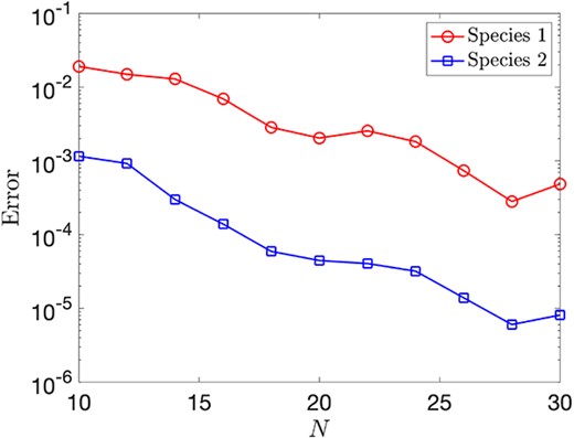
Convergence of the DDFT as |$N_{1} = N_{2} = N$| increases. Note that here ‘Error’ denotes the |$L^{2}$| relative error (in space and time) between the solution and that computed with |$N=40$| points, which we take as a reference, ‘exact’ solution.
4.2 Control problems with nonlocal PDE constraints
Finally, we are interested in solving a control problem involving the dynamics of a system of two interacting species of particles, such as that in (4.3). Here the challenge is to apply a control to the system, which is governed by the DDFT model, so that the state approximates a desired ‘target’ state, whilst also balancing the ‘cost’ of the control. This leads to a particularly complicated system of four PDEs, with several convolution integrals describing the different interactions. This can be solved by combining MultiShape with a recently-developed Newton–Krylov algorithm Güttel & Pearson (2022) for nonlinear optimization problems.
The extended formalism to tackle nonlocal problems has been introduced in Aduamoah et al. (2022) for single species systems on rectangular domains and is extended in this subsection to multiple species on a multishape domain. Overviews of PDE-constrained optimization are given in, e.g., Hinze et al. (2009); Tröltzsch (2010); De los Reyes (2015). For a system of |$n_{s}$| species, we can formulate the following control problem:
subject to the following system of |$n_{s}$| PDE constraints, for |$a = 1,...,n_{s}$|:
where |$T>0$|. Note that the difference between the system of PDE constraints above and the system (4.3) is the additional term involving |$\vec w$|. This term models how a particle distribution |$\rho _{a}$| may be influenced by a background flow |$\vec w$|.
In this optimization problem, the aim is to drive the particle distributions |$\rho _{a}$| closer to some desired states |${\widehat \rho }_{a}$|, which can be achieved by modifying |$\vec w$|, the control variable. Note that in DDFT, |$\vec w$| is generally of the form |$\vec w = \nabla V$|, where |$V$| is an external potential; see te Vrugt et al. (2020) for a discussion on considerations of other forms of |$\vec w$| and their limitations. Enforcing this condition in a control setting is more complicated, however, since enforcing the gradient of the quantity we aim to control is a problem without a unique solution for |$V$|. At present, we restrict ourselves to control via a general |$\vec w$| as a test case for the methodology. The regularization parameter |$\beta $| describes how much the use of control is penalized when solving the system and consequently how close each |$\rho _{a}$| can be driven to the targets |${\widehat \rho }_{a}$|. This minimization is subject to the physical constraints described by the system of PDEs and the corresponding boundary conditions.
We consider an optimize-then-discretize approach for this problem, so we may work with a coupled system of nonlinear PDEs within the MultiShape framework, rather than performing an outer linearization step within the optimization routine. We highlight that we do not consider theoretical questions such as uniqueness and regularity of solutions here, but rather provide a proof-of-concept that MultiShape may be tailored to nonlinear control problems. The optimization problem (4.7) can be solved by considering the corresponding first-order optimality system, applying the working in (Aduamoah et al., 2022, Section 3). It consists of the system of PDE constraints (4.8) and the adjoint PDE system where, for each species |$a$|, we have the following PDE for the adjoint variable |${q}_{a}$|:
with boundary condition |$\frac{\partial{q}_{a}}{\partial n} = 0$| and final time condition |${q}_{a}(\vec x,T) = 0$|. Note that to obtain the adjoint equation in the above form we have used that |$V_{a,b}$| is an even function, hence that |$\nabla V_{a,b}$| is an odd function, resulting in the opposite signs in the integral terms. We also assume that |$V_{a,b} = V_{b,a}$| for all |$a$| and |$b$|. The final part of the first-order optimality system is a single control, or gradient, equation
This system of PDEs for the densities and adjoints (|$\rho _{a}$| and |${q}_{a}$|) is solved by combining the MultiShape methodology with a Newton–Krylov algorithm, introduced in Güttel & Pearson (2022) and extended to nonlocal problems with nonlinear controls in Aduamoah et al. (2022)—we refer to these references for detailed descriptions. The idea of the algorithm is that a residual vector function is constructed based on the integral in time of the residuals of the state and adjoint equations, defined at every time step. The integrals are approximated using Chebyshev interpolation, not on the space, but on the time grid, whereupon the residual vector is supplemented by the misfit between the computed and exact initial/final-time conditions. This allows us to construct the Jacobian via spatial discretization at each time step, whereupon the resulting Newton systems are approximately solved using the GMRES method Saad & Schultz (1986) in combination with a Kronecker-product based preconditioner for the Schur complement matrix. We show numerical results for such a problem in Section 4.2.1. Note that this problem is of the form (2.1), when setting |$u = [\{\rho _{a}\}, \{q_{a}\}]$| and |$f = [\{f_{a}^{\text{st}}\},\{f_{a}^{\text{adj}}\}]$|, for |$a,b = 1,2,...,n_{s}$|, where |$f_{a}^{\text{st}}$| represents the right-hand side of (4.8), the state equation and |$f_{a}^{\text{adj}}$| the right-hand side of (4.9), the adjoint equation. Furthermore, the initial condition is replaced with a final time condition for the |$q_{a}$|.
4.2.1 Time-dependent solution
We compute the solution to the flow control problem (4.7), by solving the system (4.8)–(4.10) on four elements forming the shape of a bifurcated channel, with |$N_{1} = N_{2} = 14$| discretization points in space on each element and |$n = 10$| points in the time interval |$t \in [0,5]$|; see Fig. 14. We note that the normal vector at the intersection of the four elements has to be correctly defined in a manual fashion, as illustrated for a simpler test case in Fig. 2.
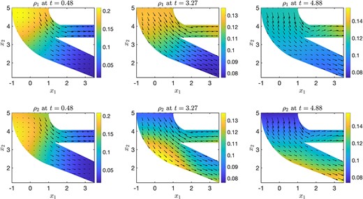
Optimal states |$\rho _{1}$| and |$\rho _{2}$| with superimposed control |$\vec w$|.
We choose two interacting particle species with |$V_{a,b}$| defined in (4.2), with relative interaction ranges and strengths given by |$\sigma _{1,1} = 0.5$|, |$\sigma _{2,2} = 1$|, |$\sigma _{1,2} = \sigma _{2,1} = 0.75$|, |$\kappa _{1,1} = -0.8$|, |$\kappa _{2,2} = -0.3$|, |$\kappa _{1,2} = \kappa _{2,1} = 0.4$|. Additionally, an external potential is imposed for each species: |$V_{\text{ext},1} =0.05 \left (\exp{(-0.1(x_{1}-2)^{2} - 0.1(x_{2}-1)^{2})} - x_{2}\right )$| and |$V_{\text{ext},2} =0.1 \left (\exp{(-0.3(x_{1}-3)^{2} - 0.3(x_{2}-4)^{2})} \right. \left.+ 2x_{2}\right )$|. The initial conditions for |$\rho _{1}$| and |$\rho _{2}$| are defined by (4.6), where in this case |$f_{1,\text{ic}} = f_{2,\text{ic}} = \exp{(-0.15(x_{1}+0.5)^{2} - 0.15(x_{2}-5)^{2})}$| and |$c_{M} = 1$|. We choose |$\beta = 10^{-3}$|, allowing a significant amount of control to be introduced into the system, so that we expect to get reasonably close to the target states |${\widehat \rho }_{1}$| and |${\widehat \rho }_{2}$|. The targets are defined by a forward problem with the same initial conditions and external potential, with a background flow of strength |$0.1$| in the |$x_{1}$| direction (along the channel in the wedge case). Without imposing control (i.e., with |$\vec w = \vec 0$|), we can evaluate the cost functional (4.7), which results in |$\mathcal J_{\text{uc}} = 0.0038$| (‘uc’ referring to ‘uncontrolled’). The value of the cost functional for the controlled system is |$\mathcal J_{\text{c}} = 1.7483 \times 10^{-4}$|, showcasing that the overall cost obtained is significantly reduced when the control is introduced.
We can observe that both species of particles are carried along by the background flow field (control) over time. Since Species |$1$| experiences an upward force, it accumulates in the top-right part of the channel system at later times. Equivalently, since Species |$2$| experiences a downward acting force, it accumulates in the bent part of the channel on the bottom right at later times of the simulation. It takes around |$3$| hours to solve this control problem, which converges within |$10$| iterations of the Newton–Krylov algorithm, to a residual error of order |$10^{-13}$| and |$10^{-15}$| for the state and adjoint variables, respectively.
5. Conclusions
In this paper, we have presented a new spectral element methodology, which allows for the efficient solution of (integro-)PDE models on complicated domains, including the application of nonlinear and nonlocal boundary conditions. A general numerical framework has been introduced, building on the existing code library 2DChebClass for pseudospectral methods, and with a specific emphasis on user-friendly features, such as the simple application of matching and boundary conditions. After successful validation of the MultiShape methodology, nontrivial numerical examples were presented, including steady state and time-dependent problems in DDFT, and in optimization involving PDEs, showcasing the power of the spectral element formalism. These examples have been chosen in view of their relevance to various industrial processes, as well as phenomena in physics and biology. There are many possible extensions to this work, such as applying the MultiShape methodology to solve more complicated DDFT models, capturing effects such as sedimentation, hydrodynamic interactions or inertia. Further future challenges include modelling and optimization of industrial processes, for example, in manufacturing and production. Other areas of research, which could potentially benefit from applying the MultiShape methodology, include models of pedestrian dynamics, brewing and spread of diseases on complicated domains.
Acknowledgments
B.D.G. and R.M.-W. would like to thank Tim Hurst, Andreas Nold and Serafim Kalliadasis for helpful discussions. The authors would like to thank Bernhard Heinzelreiter for helpful comments on the manuscript and two anonymous referees for valuable suggestions.
Funding
Maxwell Institute Graduate School in Analysis and its Applications (Engineering and Physical Sciences Research Council, EPSRC grant EP/L016508/01 to J.C.R.), the Scottish Funding Council, Heriot-Watt University and The University of Edinburgh; EPSRC (EP/W522648/1 to J.C.R.); EPSRC (grant EP/L025159/1 to B.D.G.); EPSRC Impact Acceleration Account (IAA) (PIII075 to R.M.-W.); EPSRC (grant EP/S027785/1 to J.W.P.).
Footnotes
We apply the convention that ‘MultiShape’, with capital letters, refers to our methodology as a whole, while a lower-case ‘multishape’ refers to an individual shape (i.e., domain).
For consistency with the cost functional (4.7), we adopt the notation |$\mathcal{F}(\{\rho _{b}\})$|. However, we note that |$\mathcal{F}[\{\rho _{b}\}]$| is the standard notation in the DDFT community, explicitly denoting the functional dependence on |$\{\rho _{b}\}$|.
References
A. Picard iteration for DDFT equilibria
Algorithm A.1 illustrates the Picard scheme, given initial guesses for the particle distributions |$\rho _{1,\text{ig}}$|, |$\rho _{2,\text{ig}}$|, an error tolerance to terminate the algorithm and a mixing parameter |$\lambda $| for the Picard step. The Picard step takes a linear combination of the previous and new guesses for |$\rho _{1}$|, |$\rho _{2}$|, which is designed to stabilize the algorithm. The error measure in this algorithm is defined as the maximum of the error across all species, individually computed using (3.1), with |$f_{\text{Num}}$| and |$f_{\text{Ex}}$| replaced by |$\rho _{j,\text{new}}$| and |$\rho _{j,\text{old}}$|, respectively, for |$j \in \{1,2\}$|. A numerical example of this formulation can be seen in Section 4.1.1.

