


Abstract
The existing discrete variational derivative method is fully implicit and only second-order accurate for gradient flow. In this paper, we propose a framework to construct high-order implicit (original) energy stable schemes and second-order semi-implicit (modified) energy stable schemes. Combined with the Runge–Kutta process, we can build high-order and unconditionally (original) energy stable schemes based on the discrete variational derivative method. The new energy stable schemes are implicit and leads to a large sparse nonlinear algebraic system at each time step, which can be efficiently solved by using an inexact Newton-type solver. To avoid solving nonlinear algebraic systems, we then present a relaxed discrete variational derivative method, which can construct second-order, linear and unconditionally (modified) energy stable schemes. Several numerical simulations are performed to investigate the efficiency, stability and accuracy of the newly proposed schemes.
1. Introduction
Many physical problems, such as interface dynamics Anderson et al. (1998); Lowengrub & Truskinovsky (1998); Liu & Shen (2003), crystallization Elder et al. (2002, 2007); Wei et al. (2019), thin films Giacomelli & Otto (2001), polymers Fraaije (1993); Fraaije et al. (1997); Maurits & Fraaije (1997), binary alloys Cahn & Novick-Cohen (1994); Zhang et al. (2016); Huang et al. (2020), and liquid crystals Leslie (1979); Forest et al. (2004), can be modeled by gradient flow type partial differential equations. Gradient flows are driven by a free energy functional and can be written in the following general form:
where |$\phi :=\phi (\mathbf x,t)$|, |$\varOmega \in \mathbb{R}^{d}$| with |$d=1,2,$| or |$3$| is the computational domain, |$\mathcal E\,[\phi ]$| is a given total free energy functional and |$\frac{\delta{\mathcal E}}{\delta \phi }$| is the variational derivative. The free energy functional usually can be written explicitly as
where |$\left <\varphi ,\,\psi \right>=\int _{\varOmega } \varphi \psi \,\mathrm{d} \mathbf x$|, |$\gamma $| is an interface energy coefficient and |${\mathcal E}_{1}(\phi )$| is a body free energy functional. To simplify the presentation, we only consider the well-known Ginzburg–Landau free energy functional
where |$\epsilon $| is a small parameter.
In (1.1), the operators |${\mathcal G}$| are set as |$-I$|, |$\varDelta $| and |$-(-\varDelta )^{\alpha }$| with |$(0<\alpha <1)$| for dissipation mechanisms including |$L^{2}$|, |$H^{-1}$| and |$H^{-\alpha }$| gradient flows, respectively. Assuming |${\mathcal G}$| is nonpositive, the gradient flow system satisfies the following energy dissipation law:
To simplify the presentation, we use periodic boundary conditions or homogeneous Neumann boundary conditions such that all boundary terms will vanish when integration by parts is performed.
For a gradient flow, it is very important to construct an efficient and accurate numerical method, which preserves the energy dissipation law at the discrete level. There exist several popular approaches, such as the convex splitting method Elliott & Stuart (1993); Eyre (1998); Shen et al. (2012); Baskaran et al. (2013), the stabilization method Zhu et al. (1999); Shen & Yang (2010), the exponential time differencing Ju et al. (2015); Zhang et al. (2016), the invariant energy quadratization (IEQ) Yang (2016); Zhao et al. (2017), the scalar auxiliary variable (SAV) Shen et al. (2018, 2019), the discrete variational derivative (DVD) method Du & Nicolaides (1991); Furihata & Matsuo (2011); Wei et al. (2019); Huang et al. (2020); Huang & Yang (2022), and so on. Most of them are implicit and semi-implicit second-order schemes. In contrast to fully implicit methods, semi-implicit methods only require solving a linear system at each time step, which is easier to implement and less computationally expensive. In recent years, many researchers focus on designing higher-order energy stable schemes, such as Shin et al. (2017); Akrivis et al. (2019); Gong et al. (2020); Lee et al. (2022); Yang et al. (2022). In Akrivis et al. (2019) and Gong et al. (2020), high-order and unconditionally (modified) energy stable schemes are proposed based on the SAV and IEQ method, respectively. In Shin et al. (2017) and Lee et al. (2022), high-order and unconditionally (original) energy stable schemes are constructed by using the convex splitting method. According to the collocation-type methods and SAV method, arbitrarily high-order maximum bound preserving schemes are build in Yang et al. (2022) to solve the Allen–Cahn (AC) equation. Without any additional assumptions, the DVD method, originally proposed in Du & Nicolaides (1991), can build a second-order implicit scheme for gradient flows with complicated total free energy functional, such as total free energy functional of logarithmic type Huang et al. (2020) and including elastic energy Huang & Yang (2022). However, the construction of implicit and energy stable schemes of order higher than 2 or semi-implicit linear schemes based on the DVD method has remained open.
For general gradient systems |$\dot{\phi }=-\nabla{U}(\phi )$|, the discrete gradient method is proposed to preserve the first integral McLachlan et al. (1999); Cohen & Hairer (2011); Dahlby et al. (2011); Norton & Quispel (2013); Hairer & Lubich (2014). The discrete gradient method finds a discrete gradient |$\bar{\nabla } U$| satisfying
Well-known discrete gradients are the midpoint discrete gradient (second-order Gonzalez (1996)) and the average vector field (second-order McLachlan et al. (1999) and high-order Cohen & Hairer (2011); Dahlby et al. (2011); Norton & Quispel (2013)). The average vector field used in McLachlan et al. (1999); Dahlby et al. (2011); Norton & Quispel (2013) is defined as
For given |$0\leq c_{1}\leq \cdots \leq c_{\nu }\leq 1$|, with the definition of the average vector field, the energy-preserving integrator for the gradient system (1.5) can be defined as
where |$h$| is the time step size, |$t_{0}$| is the initial time, |$\dot{u}(t_{0}+\tau h)=\sum \limits _{i=1}^{\nu } \frac{ l_{i}(\tau )}{b_{i}}\int \limits _{0}^{1} l_{i}(\tau )\nabla U\big (u(t_{0}$| |$+\tau h)\big )\,{\textrm{d}}\tau $| is a polynomial of degree |$\nu $|, |$l_{i}(\tau )$| is the Lagrange basis polynomial and |$b_{i}=\int _{0}^{1} l_{i}(\tau )\,{\textrm{d}}\tau \geq 0$|. Let us denote |$\hat{\phi }(\tau ):=u(t_{0}+\tau h)$| as the approximate solution of the gradient system |$\dot{\phi }=-\nabla{U}(\phi )$|. By taking integration of |$\dot{u}(t_{0}+\tau h)$|, we have
The numerical solution after one time step is then defined by |$\hat \phi (1)=u(t_{0}+h)$|. Following the idea of McLachlan et al. (1999), Dahlby et al. (2011) and Norton & Quispel (2013), according to (1.7) and (1.8), we have
which immediately yields energy-preserving property of the integrator (1.7) for any |$h>0$|.
The equation (1.8) represents a nonlinear system of |$\hat \phi (\tau )$|, which usually can not be solved analytically. In the discrete gradient methods, the unknown function |$\hat \phi (\tau )$| is approximated by a polynomial of degree |$\nu $|, which can be expressed in terms of |$\hat \phi (0)$|, |$Y_{1}=\hat \phi (c_{1} h)$|,..., and |$Y_{\nu }=\hat \phi (c_{\nu } h)$|. For |$U$| with polynomial forms, according to (1.8), one can obtain a |$\nu $| stage scheme for |$\hat \phi (0)$|, |$Y_{1}$|,..., and |$Y_{\nu }$|, which is similar to the implicit Runge–Kutta method and can be written as:
However, for |$U$| including non-polynomial forms, such as logarithmic function (widely used in phase field model), it is difficult (not obvious) to convert the discrete gradient method (1.8) to a scheme which can be accurately implemented (without further approximation), such as (1.10). If equation (1.8) is solved approximately, the energy-preserving property (1.9) should be relaxed to
where |${\mathcal R}_{\nu }(h)$| is the truncation error coming from the polynomial approximation of |$\hat \phi (\tau )$|. An example will be given in the Appendix A to verify the existence of the truncation error |${\mathcal R}_{\nu }(h)$|. By using the discrete gradient method with the average vector field, the truncation error also makes the energy dissipation law is satisfied only for a reasonable large time step size (see Appendix A for more details). To the best of our knowledge, there is no existing work showing that the scheme (1.10) is energy stable and satisfies the energy dissipation law for any large time step size. In Hairer & Lubich (2014), algebraically stable and high-order implicit Runge–Kutta methods are shown to satisfy energy dissipation law for a reasonable small time step size. Thus, constructing high-order and unconditionally energy stable numerical schemes based on the discrete gradient method (without any restriction on the time step size) for the gradient flow system remains a challenging problem. This is addressed in the current paper.
In this paper, we aim to present a framework to construct high-order numerical schemes for the general phase field systems (1.1), by combining the DVD method and the implicit Runge–Kutta process. In the DVD method, the discrete variational derivative |$\mu [\phi _{i},\phi _{j}]$| for two discrete total free energy functionals |${\mathcal E}^{\,i}:={\mathcal E}\,[\phi _{i}]$| and |${\mathcal E}^{\,j}:={\mathcal E}\,[\phi _{j}]$| is defined as a solution of the following equation:
where |$\phi _{i},\,\phi _{j}$| are two solutions of gradient flow (1.1) at different times. According to the definition of discrete variational derivative |$\mu [\phi _{i},\phi _{j}]$|, the DVD scheme can be viewed as a discrete gradient method with midpoint discrete gradient. As mentioned before, there is no existing high-order discrete gradient methods with midpoint discrete gradient. Therefore, the framework proposed in this paper is different from existing discrete gradient methods. The newly proposed scheme is unconditionally stable and satisfies the energy dissipation law for any large time step size if a sufficient condition is satisfied. Following the idea of the Runge–Kutta method, we can construct higher-order DVD schemes by solving a semidefinite programming (SDP) problem such that the sufficient condition is satisfied. As compared the discrete gradient method (1.8), the newly proposed high-order DVD schemes is easily extended to gradient flow system with more complex free energy functional, such as free energy functional including logarithmic function. Due to the nonlinearity of the free energy functional |${\mathcal E}$|, the higher-order numerical scheme built by using the framework is fully implicit, which is hard to implement and computationally expensive compared to linear schemes. To construct a semi-implicit linear scheme, we should choose the discrete variational derivative |$\mu [\phi _{i},\phi _{j}]$| as a linear functional of |$\phi _{i}$|. By relaxing the formula (A.2), we propose a relaxed DVD method to build a semi-implicit linear scheme. As compared with the IEQ method and the SAV method, the newly proposed relaxed DVD method is more efficient.
The remainder of this paper is organized as follows: In Section 2, we introduce a framework to construct higher-order implicit unconditionally energy stable schemes. In Section 3, we propose the relaxed DVD method to build semi-implicit linear scheme. In Section 4, we discuss the fully discrete scheme and corresponding linear/nonlinear solvers. Several numerical simulations are reported in Section 5 and the paper is concluded in Section 6.
2. A framework for constructing high-order energy stable schemes
In this section, we introduce a framework to construct a higher-order, implicit and unconditionally energy stable scheme for general gradient flows (1.1) by combining the DVD method and the implicit Runge–Kutta process.
2.1 Runge–Kutta Processes
First, we briefly review the Runge–Kutta processes Butcher (1963, 2016), which can construct a temporal discretization of the gradient flow system (1.1). Let us rewrite the gradient flow system (1.1) to be an initial value problem specified as follows:
In this paper, we assume that |$f(\phi ,t)=f(\phi (t))$|. For a given time step size |$h>0$|, a |$\nu $| stage Runge–Kutta Process obtains an approximate solution |$\phi _{\nu }$| at |$t=t_{0}+h$| by using the following equations:
where |$a_{ij},\,b_{i}$|, |$(i,\,j=1,\,2,\,\cdots ,\, \nu )$| are numerical constants. For convenience we shall designate the process by an array as the following Butcher tableau:
with |$c_{i}=\sum _{j=1}^{\nu } a_{ij} $|. The Runge–Kutta Process (2.2) is called ‘semi-implicit’ if |$a_{ij}=0$| for |$i<j$|. In particular, if additionally |$a_{ii}=0$|, the Runge–Kutta Process (2.2) is called ‘explicit’. In contrast to the ‘semi-implicit’ and ‘explicit’ processes, the Runge–Kutta Process (2.2) is called ‘implicit’ if there exists |$a_{ij}\neq 0$| for |$i<j$|. The numerical constants |$a_{ij},\,b_{i}$| and |$c_{i}$| can be determined by following the integration process of evaluating |$\int \limits _{t_{0}}^{t_{0}+c_{i}h}f(\phi ,t)\,\mathrm d t$|, such as the Gauss–Legendre quadrature formulae and the Newton–Cotes formulae Quarteroni et al. (2010).
2.2 High-order and unconditionally energy stable DVD schemes
It is easy to build an arbitrary high-order scheme for the gradient flow (1.1) by using the Runge–Kutta process. However, most of them are not unconditionally energy stable. To overcome the difficulty, we propose a framework to construct high-order and unconditionally energy stable schemes based on the DVD method. The DVD method was originally proposed in Du & Nicolaides (1991), and then used to solve phase field crystal equation Wei et al. (2019), AC/CH equations Huang et al. (2020) and Ni-based alloys system Huang & Yang (2022). The DVD methods in Du & Nicolaides (1991), Huang et al. (2020) and Huang & Yang (2022) are only second-order accurate in time. It is non-trivial to construct a high-order scheme by using the DVD method. To do it, let us first introduce some necessary notations and definitions. Assume that the time interval |$[0,T]$| is divided into |$T/h$| subintervals |$[t_{(n)},\,t_{(n+1)}]$| with |$h$| being the time step size and |$t_{(n)}=nh$|. At the |$n$|th time step, for given constants |$0\leq c_{i}\leq 1$| |$(i=1,\,\cdots ,\, \nu )$| with |$c_{\nu }=1$|, let |$\phi _{i}\approx \phi (\mathbf{x},\,t_{(n)}+c_{i} h)$| represent the approximate solutions for the gradient flow (1.1) at |$t=t_{(n)}+c_{i} h$|. The corresponding discrete total free energy is denoted as |${\mathcal E}^{\,i}:={\mathcal E}\,[\phi _{i}]$|. For ease of description, we use |${\mathcal E}_{(n)}$| and |$\phi _{(n)}$| to denote the discrete total free energy and solution at time |$t_{(n)}$|, respectively.
For two discrete total free energy functionals |${\mathcal E}^{\,i}$| and |${\mathcal E}^{\,\,j}$|, we define the discrete variational derivative |$\mu [\phi _{i},\phi _{j}]$| as a solution of the following equation:
According to the definition of total free energy (1.2), we can derive the discrete variational derivative |$\mu [\phi _{i},\phi _{j}]$| as
where |$ E_{1}\{\phi _{i},\phi _{j}\}:= \frac{E_{1}[\phi _{i}]-E_{1}[\phi _{j}]}{\phi _{i} - \phi _{j}}$| is the first-order finite quotient of functional |$E_{1}$|. If the energy functional |$E_{1}$| is a polynomial function of |$\phi $|, the first-order finite quotient |$ E_{1}\{\phi _{i},\phi _{j}\}$| is also a polynomial function of |$\phi _{i}$| and |$\phi _{j}$|. For the energy functional |$E_{1}$| containing a non-polynomial function of |$\phi $|, such as logarithmic type functional, the first-order finite quotient |$ E_{1}\{\phi _{i},\phi _{j}\}$| is no longer a polynomial function of |$\phi _{i}$| and |$\phi _{j}$|. In this situation, the numerical computation of the first-order finite quotient |$E_{1}\{\phi _{i},\phi _{j}\}$| is unstable and inaccurate when |$\phi _{i}-\phi _{j}$| is close to zero. Unfortunately, in phase field systems, |$\phi _{i}-\phi _{j}$| is often close to zero, which indicates that the numerical calculation of |$ E_{1}\{\phi _{i},\phi _{j}\}$| is numerically unstable and inaccurate. To overcome the difficulty, a stable and highly accurate approximation for the first-order finite quotient |$ E_{1}\{\phi _{i},\phi _{j}\}$| was proposed in Huang et al. (2020) and Huang & Yang (2022). For ease of presentation, we focus on the double well potential, that is |$E_{1}(\phi )= \frac 1 {4\epsilon ^{2}}(1-\phi ^{2})^{2}$|. The first-order finite quotient |$ E_{1}\{\phi _{i},\phi _{j}\}:= \frac{E_{1}[\phi _{i}]-E_{1}[\phi _{j}]}{\phi _{i} - \phi _{j}}$| is defined as
Let us denote vectors |$\mathbf{y}=(\mu [\phi _{1},\phi _{0}],\,\mu [\phi _{2},\phi _{0}],\,\cdots ,$| |$\mu [\phi _{\nu },\phi _{\nu -1}])^{T}\in \mathbb{R}^{\hat \nu }$| and |$ \overrightarrow{\delta \phi }=(\phi _{1}-\phi _{0},\,\phi _{2}-\phi _{0},\,\cdots ,\,{ {\phi _{\nu }-\phi _{0},}}\,\phi _{2}-\phi _{1},\,\phi _{3}-\phi _{1},\,\cdots ,\,{ {\phi _{\nu }-\phi _{1},\,\phi _{3}-\phi _{2},}}\,\cdots \phi _{\nu }-\phi _{\nu -1})^{T}\in \mathbb{R}^{\hat \nu }$| with |$\hat \nu =\frac{\nu (\nu +1)}{2}$|. Following the idea of the Rung–Kutta process, we define a |$\nu $| stage DVD scheme as follows:
where |$\tilde a_{ij}$|, |$(i=1,\,2,\,\cdots ,\, \nu ,\, j=1,\,2,\,\cdots ,\, \hat \nu )$| are numerical constants. For convenience we shall designate the process by an array as the following tableau:
where |$c_{i}=\sum _{j=1}^{\hat \nu }\tilde a_{ij} $|. Similar to the derivation of the Runge–Kutta method Butcher (2016), we can obtain the numerical constants |$\tilde a_{ij}$| for given |$c_{i}$| and |$\nu $|. It is important to point out that the numerical constants |$\tilde a_{ij}$| should be chosen carefully such that the proposed scheme (2.7) is unconditionally energy stable. We will discuss more details of how to determine the numerical constants |$\tilde a_{ij}$| later in this section.
For ease of presentation, let us rewrite the scheme (2.7) in the matrix form as follows:
where |$\mathbb{A}=(\tilde a_{ij})$| is a |$\hat \nu $|-order square matrix. The |$\nu +1,\, \cdots , \hat \nu $| rows of the matrix |$\mathbb{A}$| are computed by using tableau (2.8) and |$\phi _{i}-\phi _{j} = (\phi _{i}-\phi _{0})-(\phi _{j}-\phi _{0})$|. For example, due to |$\phi _{3}-\phi _{1}=(\phi _{3}-\phi _{0})-(\phi _{2}-\phi _{0})$|, we have |$\mathbb{A}(2\nu ,k)=\tilde{a}_{3k}-\tilde{a}_{2k}$| for |$k=1,\,\cdots ,\hat \nu $|. Next, we call a vector |$\mathbf{v}=(v_{1},\,\cdots ,\,v_{\hat \nu })\in \mathbb{R}^{\hat \nu }$| as a unit partition vector of |${\mathcal E}^{\,\nu }-{\mathcal E}^{\,0}$| if and only if
According to the definition of the discrete variational derivative (2.4), we have
where |$\mathbb{B}=\frac 1 2\left (\hbox{diag}(\mathbf{v})\mathbb{A}+\mathbb{A}^{T}\hbox{diag}(\mathbf{v})\right )\in \mathbb{R}^{\hat \nu \times \hat \nu }$| is a symmetric matrix.
The following theorem gives a sufficient condition such that the |$\nu $| stage DVD scheme is unconditionally energy stable.
It is easy to check that the DVD methods in Du & Nicolaides (1991), Huang et al. (2020) and Huang & Yang (2022) satisfy the sufficient condition given in Theorem 1, which is second-order accurate in time. Next, we present a strategy to construct high-order DVD schemes. For convenience of description, we only consider a |$\nu $| stage DVD scheme with |$c_{i}=i/\nu $| for |$i=0,\,\cdots ,\nu $|. The new strategy includes three stages. In the first stage, we determine the parameters |$ \tilde a_{\nu 1},\, \tilde a_{\nu 2}, \cdots ,\,\tilde a_{\nu \hat \nu }$| in (2.8) according to the accurate requirement. For a |$p$|-order DVD scheme, the accurate requirement can be written as
The standard way for the calculation of |$\tilde a_{\nu i}$| is to solve the undetermined coefficient equations based on the Taylor expansion method. In this paper, we introduce the Richardson extrapolation method Quarteroni et al. (2010) to do it, which is easer to implement. Assume that |${\mathcal I}(h)$| is an approximation of |$ \int _{0}^{h} f(\phi ,\,t)\,{\mathrm{d}}t$| of order |$p_{0}$|, then the Richardson extrapolation |${\mathcal T}(h):=\frac{{\mathcal I}(\delta h)-\delta ^{p_{0}}{\mathcal I}(h)}{1-\delta ^{p_{0}}}$| approximates |$ \int _{0}^{h} f(\phi ,\,t)\,{\mathrm{d}}t$| up to order |$p_{0}+1$| (at least). Here, |$\delta <1$| is the ratio of two mesh sizes. According to the Richardson extrapolation method, and based on the second-order DVD methods in Du & Nicolaides (1991), Huang et al. (2020) and Huang & Yang (2022), we have
and
For |$\nu>3$|, one can obtain |$\tilde a_{\nu i}$| in a similar way.
In the second stage, for any given |$\nu $|, let us denote |$t_{i}=\frac i{\nu }h$| with |$i=1,2,\cdots ,\nu $|. Based on a constructed low-order DVD scheme, we can obtain the approximation of |$ \int _{0}^{t_{i}} f(\phi ,\,t)\,{\mathrm{d}}t$|. The corresponding weight coefficients for the integral |$\int _{0}^{t_{i}} f(\phi ,\,t)\,{\mathrm{d}}t$| can be written as the following tableau:
Taking |$\nu =3$| as an example, based on the second-order DVD scheme Du & Nicolaides (1991); Huang et al. (2020); Huang & Yang (2022), the tableau (2.16) can be specifically expressed as
The tableau (2.16) can be viewed as a low-order scheme, which is usually not energy stable for the gradient flow system (2.1). In the third stage, we construct an energy stable scheme with given order based on the tableau (2.16). Let us assume that the tableau (2.8) can be rewritten as the following form:
where |$\mathbf{z}_{i}=(z_{i1},\,\cdots ,\,z_{i\tilde \nu })^{T}$| are undetermined vectors with |$i=1,\,2,\,\cdots ,\,\nu -1$| and |$\sum \limits _{j}^{\tilde \nu }z_{ij}=0$|. According to the accurate requirement, there are several potential choices of the vectors |$\mathbf{z}_{i}$|. We determine them by solving an SDP problem. Let us denote the matrix |$\mathbb{A}$| in (2.9) as |$\mathbb{A}(\mathbb Z)$| with |$\mathbb Z=(\mathbf{z}_{1},\,\cdots ,\,\mathbf{z}_{\nu -1})$|. The SDP problem we solved is an optimization problem of the form:
where |$\mathbb{B}=\frac 1 2\left (\hbox{diag}(\mathbf{v})\mathbb{A}(\mathbb Z)+\mathbb{A}(\mathbb Z)^{T}\hbox{diag}(\mathbf{v})\right )$|. After solving the SDP problem (2.19), we can obtain a |$\nu $| stage schemes by using the newly proposed framework. We list some high-order DVD schemes as following, where |$p$| denotes the order of convergence rate. More details of constructing high-order DVD schemes will be shown in Appendix B.
We complete the proof of this theorem by choosing a unit partition vector |$\mathbf{v}$| such that the matrix |$\mathbb{B}$| is positive semidefinite.
For the scheme Sch-1, we set |$\mathbf{v}=1$| and the corresponding |$\mathbb{B}=1$|.
The framework introduced in this section can generate high-order DVD schemes. We establish that the DVD scheme is unconditionally energy-stable and adheres to the original energy dissipation law without any assumptions or stabilization parameters. This stands as a significant advantage of the newly proposed high-order DVD scheme. Given the nonlinearity of the total free energy, we observe that the discrete variational derivative in (2.6) is a nonlinear function of |$\phi _{i}$|. Consequently, Schemes Sch-1–Sch-6 are nonlinear and fully implicit, resulting in nonlinear algebraic systems upon full discretization. Due to the non-convexity of the energy function |$\mathcal{E}(\phi )$|, we can only prove the unique solvability of the nonlinear algebraic system obtained by the DVD method with |$h$| on the order of |$\mathcal{O}({\varepsilon ^{2}})$|. Fortunately, these nonlinear algebraic systems are typically numerically solvable using the inexact Newton-type algorithm Cai et al. (1994), even for relatively large values of |$h$|, such as |$h=4$| (refer to the numerical results in Example 3). As reported in Huang et al. (2020) and Huang & Yang (2022), in the case of a more complex gradient flow, such as the phase field crystal system and the coupled AC/Cahn–Hilliard (CH) system, a sudden increase in the time step size has a detrimental effect on maintaining computational accuracy and may lead to divergence of the nonlinear solver. But, due to unconditionally energy stability of the DVD scheme, adaptive time stepping strategies Huang et al. (2020); Huang & Yang (2022) can adaptively choose the time step size according to the desired solution accuracy and the dynamic features of the system. Therefore, the unconditional energy stability of the DVD scheme remains crucial, even though we can only prove the unique solvability of the nonlinear algebraic system obtained by the DVD method with |$h$| on the order of |$\mathcal{O}(\varepsilon ^{2})$|.
3. The relaxed DVD method
When compared to well-known linear schemes like IEQ Yang (2016); Zhao et al. (2017) and SAV Shen et al. (2018, 2019), these nonlinear implicit schemes generated by the DVD method are more intricate and less efficient. To overcome this challenge, we introduce several relaxed DVD methods in the next section to develop linear, unconditionally energy-stable schemes for gradient flow problems. The newly proposed method is called the relaxed DVD method because the formula (2.4) for the discrete total free energy functionals and the discrete variational derivative is relaxed to construct a linear unconditionally energy stable scheme.
The first type of relaxed DVD method can be constructed by relaxing the formula (2.4) to
where the discrete variational derivative |$\mu [\phi _{i},\phi _{j}]$| should be chosen as a linear function of |$\phi _{i}$| for |$i>j$|. We then define a |$\nu $| stage relaxed DVD scheme as follows:
where |$y_{\frac{j(2\nu -j+1)}{2}+(i-j)}=\mu [\phi _{i},\phi _{j}]$|. The |$\nu $| stage relaxed DVD scheme (3.2) is a linear scheme due to the definition of the discrete variational derivative (3.1). For a non-negative unit partition vector |$\mathbf{v}$| of |${\mathcal E}^{\,\nu }-{\mathcal E}^{\,0}$|, we have
If the matrix |$\mathbb{B}$| is positive semidefinite, it is straightforward to prove that the |$\nu $| stage relaxed DVD scheme is unconditionally energy stable.
Next, we introduce an approach to select |$\mu [\phi _{i},\phi _{j}]$| satisfying (3.1) by following the idea of the stabilization method Zhu et al. (1999); Shen & Yang (2010). Let us replace the double-well potential |$E_{1}(\phi )$| by a quadratic truncated double-well potential Shen & Yang (2010). With this truncated double-well potential, there exist linear operators |$\kern4pt\hat{\!\!\!\mathcal L}$| such that both |$\kern4pt\hat{\!\!\!\mathcal L}$| and |$\kern4pt\hat{\!\!\!\mathcal L}-\frac{\delta ^{2} {\mathcal E}_{1}}{(\delta \phi )^{2}}[\phi ]$| are positive. The linear operator |$\hat{\mathcal L}$| is commonly chosen as
We then take a particular convex splitting as |${\mathcal E}\,[\phi ]:={\mathcal E}_{c}[\phi ]-{\mathcal E}_{e}[\phi ]$| with
where both |${\mathcal E}_{c}$| and |${\mathcal E}_{e}$| are convex about unknown |$\phi $|. For |$\nu =1$|, we can take the discrete variational derivative |$\mu [\phi _{1},\phi _{0}]$| as |$\frac{\delta{\mathcal E}_{c}}{\delta \phi }[\phi _{1}] - \frac{\delta{\mathcal E}_{e}}{\delta \phi }[\phi _{0}]$|. Due to the property of the convex functional
we get the following inequality:
which leads to the well known unconditionally energy stable scheme (stabilization method):
The stabilization method is first-order and can be extended to second-order schemes, but in general, it cannot be unconditionally energy stable. The relaxed DVD method gives a potential way to construct high-order unconditionally energy stable scheme.
We then propose another type of the relaxed DVD method by following the idea of the IEQ approach Yang (2016); Zhao et al. (2017). Let us rewrite the free energy functional as
where |${\mathcal L}=-\varDelta + \frac \beta{\epsilon ^{2}} $| and |$\bar{\mathcal E}_{1}(\phi ):=\int _{\varOmega }\bar{ E}_{1}(\phi )\mathbf x=\int _{\varOmega } \frac 1 {4\epsilon ^{2}}(1+\beta -\phi ^{2})^{2}\,\hbox{d}\mathbf x$|. Here |$\beta $| is a suitable stabilization parameter. Let us introduce an auxiliary variable |$Q:=Q(\phi )=\left (\bar E_{1}(\phi )+C_{0}\right )^{1/m}$|, where |$m$| is a positive integer number. For |$m=1$|, |$C_{0}$| can be any constant. For an odd integer number |$m$|, |$C_{0}$| should be a constant such that |$\bar E_{1}(\phi )+C_{0}\neq 0$|. For an even integer number |$m$|, |$C_{0}$| should be a constant such that |$\bar E_{1}(\phi )+C_{0}>0$|, which corresponds to the assumption that the energy |$\bar E_{1}(\phi )$| should be bounded from below. With the auxiliary variable |$Q$|, one can obtain a modified total free energy
For two modified discrete total free energy functionals |$\kern4pt\hat{\!\!\!\mathcal E}{}^{\,i}:=\kern4pt\hat{\!\!\!\mathcal E}\,[\phi _{i},Q_{i}]$| and |$\kern4pt\hat{\!\!\!\mathcal E}{}^{\,j}:=\kern4pt\hat{\!\!\!\mathcal E}\,[\phi _{j},Q_{j}]$| with |$Q_{j}$| being the approximation of |$Q$| at |$t=t_{0}+c_{j} h$|, we assume that the discrete variational derivative |$\mu [\phi _{i},\phi _{j}]$| is a solution of
In the left hand side of (3.8), we use modified discrete total free energy functional |$\kern4pt\hat{\!\!\!\mathcal E}{}^{\,i}$| to replace the original discrete total free energy functional |${\mathcal E}^{\,i}$|. Thus, the (3.8) can be taken as a relaxation of (2.4). For |$\nu =1$|, according to (3.7), we have the discrete variational derivative |$\mu [\phi _{1},\phi _{0}]$| taking the following form:
where |$\bar \phi _{ {1}/{2}}$| can be any explicit approximation of |$\frac{\phi _{1}+\phi _{0}}{2}$| according to the accuracy requirement. By taking |$Q_{1}-Q_{0}=\frac{\bar E_{1}^{\prime}(\bar \phi _{ {1}/{2}})}{m Q^{m-1}(\bar \phi _{ {1}/{2}})}(\phi _{1}-\phi _{0})$|, we have
which implies that (3.8) holds exactly with the discrete variational derivative given by (3.9). Finally, we can define a new type of relaxed DVD scheme as follows:
According to (3.8), (3.9) and (3.11), the unconditional (modified) energy stability of scheme (3.11) is obtained by
For |$m=2$|, the scheme (3.11) is the same as the IEQ/CN scheme.
The relaxed DVD scheme (3.11) is linear and unconditionally stable for general gradient flows, which is constructed by following the idea of the IEQ scheme. In the IEQ scheme, the energy density |$\bar E_{1}(\phi )$| should be bounded from below, which limits the application of the IEQ scheme. But, the relaxed DVD scheme (3.11) with odd integer |$m$|, especially for |$m=1$|, works well for the unbounded energy density |$\bar E_{1}(\phi )$|, which should be an advantage as compared with the IEQ scheme. However, the linear system usually involves field variable coefficients, which is larger than the original linear problem. This is the same disadvantage as the IEQ scheme. To overcome it, we propose another relaxed DVD scheme by introducing a scale auxiliary variable similar to the SAV approach Shen et al. (2018, 2019).
Let us introduce a scale auxiliary variable |$r:=r(\phi )=\left (\bar{\mathcal E}_{1}(\phi )+C_{0}\right )^{1/m}$|. Similar to the auxiliary variable |$Q$|, we recommend using an odd integer number |$m$| in the scale auxiliary variable |$r$|, such as |$m=1$|. A modified total free energy is then defined as
For two modified discrete total free energy functionals |$\hat{\mathcal E}{}^{\,i}:=\hat{\mathcal E}\,[\phi _{i},r_{i}]$| and |$\hat{\mathcal E}{}^{\,j}:=\hat{\mathcal E}\,[\phi _{j},r_{j}]$| with |$r_{j}$| being the approximation of |$r$| at |$t=t_{0}+c_{j} h$|, the discrete variational derivative |$\mu [\phi _{i},\phi _{j}]$| is selected such that
The formula (3.14) is another relaxation of (2.4) since modified discrete total free energy functional |$\hat{\mathcal E}^{\,i}$| is used to replace the original discrete total free energy functional |${\mathcal E}^{\,i}$|. For |$\nu =1$|, according to (3.13), we can derive the discrete variational derivative |$\mu [\phi _{1},\phi _{0}]$| as
where |$\bar \phi _{ 1/{2}}$| can be any explicit approximation of |$\frac{\phi _{1}+\phi _{0}}{2}$| according to the accuracy requirement. By taking |$r_{1}-r_{0}=\frac{\left <\bar E_{1}^{\prime}(\bar \phi _{1/{2}}),(\phi _{1}-\phi _{0})\right>}{m r^{m-1}(\bar \phi _{ 1/{2}})}$|, we obtain that
which shows that (3.14) holds exactly for the discrete variational derivative given by (3.15).
A new relaxed DVD scheme is then defined as follows:
According to (3.14), (3.15) and (3.17), we have
which corresponds to the unconditional (modified) energy stability of scheme (3.17). For |$m=2$|, the scheme (3.17) is the same as the SAV/CN scheme.
In summary, we have the following theorem for all relaxed DVD schemes.
The IEQ approach and SAV approach are remarkable as they allow us to construct linear and unconditionally stable schemes for a large class of gradient flows. However, those approaches still suffer from the following drawbacks:
At each time step, the IEQ approach needs to solve a linear system involving auxiliary variables and the SAV approach needs to solve two linear equations.
For the two approaches, one needs to assume that |$\bar{\mathcal E}_{1}$| or |$\bar E_{1}$| should be bounded from below.
For gradient flows with multiple components, the IEQ approach will lead to coupled systems.
The relaxed DVD method inherits all the advantages of the IEQ and SAV approach, but also overcomes most of its shortcomings. If |$m$| is an odd integer number, we don’t need to assume that |$\bar{\mathcal E}_{1}$| or |$\bar E_{1}$| should be bounded from below. More importantly, for |$m=1$|, the relaxed DVD schemes (3.11) and (3.17) are fully decoupled schemes. At each time step, we only need to solve the first equation of (3.11) or (3.17), which corresponds to a linear system without auxiliary variables. If necessary, we can explicitly update the auxiliary variables by using the second equation of (3.11) or (3.17). The computational complexity is half that of the SAV approach and less than half that of the IEQ approach, respectively.
The relaxed DVD schemes (3.11) and (3.17) both are second-order. However, it is nontrivial to construct a high-order energy stable scheme by using the relaxed DVD method. For |$\nu>1$|, it is difficulty to find discrete variational derivatives |$\mu [\phi _{i},\phi _{j}]$| such that the equation (3.8) and (3.14) are exactly hold for |$1\leq j<i\leq \nu $|. We list it as future work. In addition, one can use a class of extrapolated and linearized Runge–Kutta method to build high-order energy stable schemes, see Akrivis et al. (2019) for more details.
4. Fully discrete scheme and linear/nonlinear solver
4.1 Fully discrete scheme
A fully discrete scheme is then constructed by discretizing the |$\nu $| stage DVD scheme (2.7) or the relaxed DVD schemes (3.5), (3.11) and (3.17) with a spatial discrete method, such as the finite difference method, the finite element method, or the spectral method. If the relationship (2.4), (3.1), (3.8) or (3.14) is still exactly held in the fully discrete level and the discretization operator of |${\mathcal G}$| is still negative semidefinite, the fully discrete scheme is unconditionally stable and satisfies the energy dissipation law. In this paper, we apply the finite difference method to discrete the |$\nu $| stage DVD scheme (2.7). The fully discrete scheme for the relaxed DVD schemes (3.5), (3.11) and (3.17) can be constructed similarly.
Without loss of generality, we take the |$H^{-1}$| gradient flow as an example to introduce the fully discrete scheme. The operator |${\mathcal G}=\varDelta $| in the |$H^{-1}$| gradient flow. A one dimensional domain |$\varOmega =[0,L_{x}]$| is covered by a uniform mesh with the mesh size |$\varDelta x = L_{x}/N_{x}$|. Let us denote |$\tilde{\phi }_{i}^{j}\approx \phi _{i}(x_{j})$| as the approximate solution |$\phi _{i}$| at |$x=x_{j}$|, where |$x_{j}= (j-\frac{1}{2})\varDelta x$| with |$1\leq j \leq N_{x}$|. Throughout the paper, notations with a tilde are the corresponding approximate solutions or functions at the discrete level. Let us introduce some useful discrete operators as follows:
The operator |$\mathcal G$| is discretized by |$[\varDelta \tilde \phi _{i}]^{j} = [D_{x}^{2} \tilde \phi _{i}]^{j}$|. With the periodic boundary conditions or the homogeneous Neumann boundary conditions, we present vital formula
which implies that the discretization operator of |$\mathcal G$| is negative semidefinite.
We then define the discrete free energy functional as
Correspondingly, we can derive the discrete variational derivative |$\tilde \mu [\tilde \phi _{i}^{j},\tilde \phi _{s}^{j}]$| as
where |$i>s$|. With the definition, we have
which implies that the formula (2.4) holds in the discrete level. Finally, the fully discrete scheme is given by
The proof for Theorem 5 is similar to the proof for Theorem 2 and will not be given in this paper.
4.2 Linear/nonlinear solver
By discretizing the gradient flow (1.1) with the proposed energy stable scheme (4.5), a discrete nonlinear equation system is constructed and required to be solved at each time step. This should be a disadvantage compared to linear schemes such as the IEQ and SAV methods since nonlinear algebraic systems are more expensive to solve than linear algebraic systems. In this paper, we solve the nonlinear system by using the inexact Newton-type algorithm Cai et al. (1994). At each time step, the nonlinear algebraic system is denoted as |${\mathcal F}(\mathbf{X})=0$|, and the unknown |$\mathbf{X}$| is organized by points, i.e. |$\mathbf{X}=(\tilde \phi ^{1}_{1},\, \tilde \phi ^{1}_{2}$|, |$\cdots ,\, \tilde{\phi }^{1}_{\nu },\,\tilde \phi ^{2}_{1},\, \tilde \phi ^{2}_{2},\,\cdots )^{T}$|. Assume |$\mathbf{X}_{m}$| is the solution at the |$m$|th Newton iteration, then a new solution |$\mathbf{X}_{m+1}$| can be obtained by the following steps:
- Compute an inexact Newton direction |$\mathbf{S}_{m}$| by solving the following Jacobian system with an iterative method:where |$J_{m}:=\nabla{\mathcal F}(\mathbf{X}_{m})$| is the Jacobian matrix at the solution |$\mathbf{X}_{m}$|.(4.6)$$ \begin{align}& \begin{array}{ll} J_{m}\mathbf{S}_{m}=-{\mathcal F}(\mathbf{X}_{m}), \end{array}\end{align} $$
Calculate a new solution through |$\mathbf{X}_{m+1}=\mathbf{X}_{m} +\lambda _{m}\mathbf{S}_{m}$|, where the step length |$\lambda _{m}\in (0,1]$| is determined by a line search procedure Dennis & Schnabel (1996).
The stopping condition for the nonlinear iteration is set as
where |$\varepsilon _{r}=10^{-12}, \varepsilon _{a} =10^{-12}$| are the relative and absolute tolerances for the nonlinear iteration, respectively.
In each time step of the relaxed DVD schemes or each iterative step of the Newton solver, we need to solve a large sparse linear system. Let us denote the linear system as |${\mathcal A}{\mathcal X}=\mathbf{b}$|. In this paper, we solve the linear system by using a restarted Generalized Minimal Residual (GMRES) method Saad & Schultz (1986) with right-preconditioner until the linear residual |$\mathbf{R} = {\mathcal A}{\mathcal X}-\mathbf{b}$| satisfies the stopping condition as follows:
Here |$\xi _{r}, \xi _{a} $| are the relative and absolute tolerances for the linear iteration, respectively. For the relaxed DVD schemes, we take the tolerances as |$\xi _{r}=10^{-12}, \xi _{a}=10^{-12} $|. In each iterative step of the Newton solver, the tolerances are set as |$\xi _{r}=10^{-14}, \xi _{a}=10^{-3} $|. The preconditioned linear system is written as
where |$H^{-1}$| is the additive Schwarz type preconditioner. In this paper, we use the standard additive Schwarz preconditioner Dryja & Widlund (1994). More comparison of the standard additive Schwarz preconditioner, the left restricted additive Schwarz Cai & Sarkis (1999) preconditioner, and the right restricted additive Schwarz Cai et al. (2003) preconditioner can be found in Wei et al. (2019), Huang et al. (2020) and Huang & Yang (2022).
5. Numerical simulations
In this section, we apply the DVD scheme (2.7), the relaxed DVD schemes (3.11) and (3.17) to solve the AC equation and CH equation. We compare six DVD schemes and two relaxed DVD schemes, whose abbreviations are given in Table 1. We mainly focus on the efficiency, stability and accuracy of the newly proposed methods. The algorithms for the phase field system are implemented on top of the Portable, Extensible Toolkits for Scientific computations (PETSc) library Balay et al. (2019). The numerical experiments are performed on the LSSC-IV supercomputer.
5.1 CH equation
The CH equation is an |$H^{-1}$| gradient flow and reads as
(Convergence rate of the newly proposed schemes for the standard CH equation). The computational domain is set as |$(0,\,2\pi )^{2}$|, which is covered by a |$500\times 500$| uniform mesh. The parameters |$\epsilon = 0.1$| and |$\gamma =1$|. The initial data is chosen as: |$\phi (\mathbf{x},0)=0.05 \sin x_{1} \sin x_{2}$|. The stabilization parameter |$\beta $| is chosen as 1. In the relaxed DVD scheme (3.17), |$\bar \phi _{n+1/2}=\frac 3 2 \phi _{n}-\frac 1 2\phi _{n-1}$|. The numerical solutions at |$t=0.01$| obtained by using |$\varDelta t$| sufficiently small are taken as the reference solutions. The numerical errors at |$t=0.01$| for eight schemes are shown in Table 2, from which we can observe the idea convergence rate for all schemes, except for the scheme Sch-6. As the schemes Sch-3, Sch-4, Sch-5 and Sch-6 all are numerically fourth-order, we only report the results of the schemes Sch-3 and Sch-4 in the following section While the Sch-1, R-DVD-1 and SAV/CN schemes are second-order accurate, the numerical error of the implicit scheme ( Sch-1) is an order of magnitude smaller than that of the other two semi-implicit schemes (R-DVD-1, and SAV/CN). We further compare the efficiency of the three second-order schemes. The time step size is set as 1e-4 for the implicit scheme (Sch-1) and 2.5e-5 for the other two second-order semi-implicit schemes (R-DVD-1, and SAV/CN), such that the numerical errors coming from the three second-order schemes are almost the same. The total computing times and the linear/nonlinear iteration numbers are shown in Table 3. It can be observed that the computation time per time step of the R-DVD-1 scheme is almost half that of the other two schemes due to the lowest computational complexity per time step. However, due to the accuracy advantage, the implicit scheme (Sch-1) outperforms other second-order schemes in the total computing time. It is worth to point out that the performance of the nonlinear and linear schemes is implementation dependent. For the gradient flow system with constant mobility, the performance of linear schemes can be greatly improved by employing fast Fourier Transform or LU decomposition.
Errors and convergence rates of the DVD schemes and the relaxed DVD schemes for the CH equation
| Scheme | |$h$| | 1e-4 | 5e-5 | 2.5e-5 | 1.25e-5 |
|---|---|---|---|---|---|
| Sch-1 | Error | 1.95e-4 | 4.79e-5 | 1.08e-5 | 1.78e-6 |
| Rate | — | 2.02 | 2.15 | 2.59 | |
| R-DVD-1 | Error | 3.42e-3 | 8.71e-4 | 2.21e-4 | 5.34e-5 |
| Rate | — | 1.97 | 1.98 | 2.05 | |
| SAV/CN | Error | 3.43e-3 | 8.75e-4 | 2.22e-4 | 5.36e-5 |
| Rate | — | 1.97 | 1.98 | 2.05 | |
| Scheme | |$h$| | 5e-4 | 2.5e-4 | 1.25e-4 | 6.25e-5 |
| Sch-2 | Error | 2.09e-4 | 1.48e-5 | 1.75e-6 | 2.18e-7 |
| Rate | — | 3.82 | 3.09 | 3.00 | |
| Sch-3 | Error | 2.10e-4 | 1.24e-5 | 7.72e-7 | 4.88e-8 |
| Rate | — | 4.08 | 4.01 | 3.98 | |
| Sch-4 | Error | 9.05e-5 | 5.43e-6 | 3.34e-7 | 1.98e-8 |
| Rate | — | 4.06 | 4.01 | 4.08 | |
| Sch-5 | Error | 5.05e-05 | 3.05e-06 | 1.89e-07 | 1.12e-08 |
| Rate | — | 4.05 | 4.01 | 4.08 | |
| Sch-6 | Error | 1.00e-6 | 1.13e-7 | 1.04e-08 | 7.18e-10 |
| Rate | — | 3.15 | 3.45 | 3.85 |
The total linear/nonlinear iterations and total computing time of the Sch-1, R-DVD-1 and SAV/CN for the CH equation. All simulations are run by using 144 processors
| Scheme | |$h$| | Error | Time steps | Newton | GMRES | Computing time (s) |
|---|---|---|---|---|---|---|
| Sch-1 | 1e-4 | 1.95e-4 | 100 | 341 | 5,697 | 18.07 |
| 2.5e-5 | 1.08e-5 | 400 | 1,200 | 21,271 | 71.13 | |
| R-DVD-1 | 2.5e-5 | 2.21e-4 | 400 | − | 12,374 | 33.87 |
| SAV/CN | 2.5e-5 | 2.22e-4 | 400 | − | 25,780 | 72.38 |
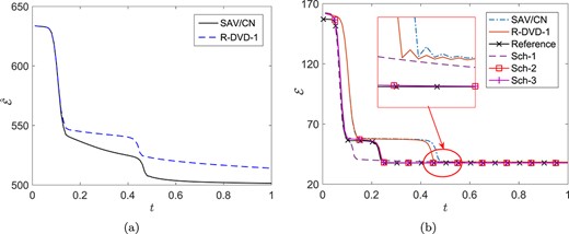
(Stability verification of the newly proposed schemes for the standard CH equation). The computational domain is set as |$\varOmega =(0,\,2\pi )$|, which is covered by a uniform mesh with mesh size being |$\pi /250$|. The parameter |$\epsilon = 0.1$|, and |$\gamma =1$|. In the relaxed DVD scheme (3.17), |$\bar \phi _{n+1/2}=\frac 3 2 \phi _{n}-\frac 1 2\phi _{n-1}$|. The initial condition is |$\phi (x,\,0)=0.2\sin x$|. The numerical solutions at |$T=0.01$| are plotted in Fig. 1(a)–(b). The implicit scheme Sch-1 can get an accurate solution with time step size |$h=5\times 10^{-4}$|, while the other second-order semi-implicit schemes have less accurate solutions. With a large time step size |$h=10^{-3}$|, the high-order DVD scheme (Sch-2, Sch-3, Sch-4) can get accurate solutions, while the second-order implicit/semi-implicit schemes are inaccurate. The numerical solutions at |$T=0.1$| are plotted in Fig. 1(c–d). For a large time step size |$h=10^{-3}$|, we find that the four implicit schemes (Sch-1,..., Sch-4) are unconditionally stable and the semi-implicit schemes (R-DVD-1 and SAV) are stable with a suitable parameter |$\beta $|. The evolutions of the modified total free energy for the semi-implicit schemes (R-DVD-1 and SAV) are given in Fig. 2-(a), which validates the unconditional (modified) energy stability of the semi-implicit schemes. However, the semi-implicit schemes do not satisfy the (original) energy dissipation law, as shown in Fig. 2-(b). The dynamic processes of the high-order implicit schemes (Sch-2, Sch-3, Sch-4) agree well with the reference dynamic process obtained by the SAV/CN scheme with a small time step size |$h=0.00002$|. In contrast, the results obtained by the second-order schemes are visibly different from the reference dynamic process.
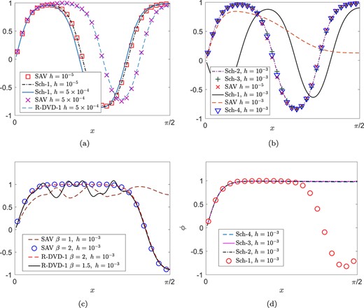
Numerical solutions of |$\phi $| in |$(0,\pi /2)$| at different time. (a) |$T = 0.01$|. |$h = 5\times 10^{-4}$|. (b) |$T = 0.01$|. |$h = 10^{-3}$|. (c) |$T = 0.1$|. |$h= 10^{-3}$|. (d) |$T = 0.1$|. |$h= 10^{-3}$|.
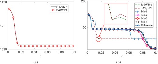
Time step size |$h=0.001$| and |$\beta =2$|. Here reference solution is obtained by the SAV/CN scheme with a small time step size |$h=0.00002$|. (a) Modified total free energy |$\hat{\mathcal E}$|. (b) Original total free energy |${\mathcal E}$|.
5.2 AC equation
The AC equation we solved is an |$L^{2}$| gradient flow given by
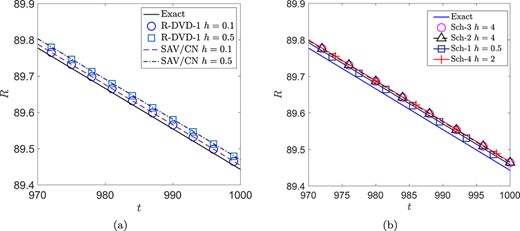
The evolution of radius |$R(t)$|.
The computational domain is set as |$(0,\,2\pi )$|, which is covered by a uniform mesh with mesh size being |$\pi /250$|. The parameters in AC equation are taken as |$\epsilon = 0.1$| and |$\gamma =1$|. The initial data is set to be a randomly distributed state |$\phi (\mathbf{x},0)=\delta _{\phi }$|, where |$\delta _{\phi }$| is a uniform random distribution function of |$0.02$| to |$0.02$|. The numerical solutions obtained by using SAV/CN with a sufficiently small |$h=0.005$| are taken as the reference solutions. We plot the numerical solutions at |$t=0.1$| and |$t=1$| using the newly proposed schemes with a large time step size |$h=0.01$| in Fig. A.1. The numerical results of all schemes agree well with the reference solution at |$t=1$|, but the solutions obtained by the semi-implicit schemes (R-DVD-1 and SAV/CN) have visible differences with the reference solution at |$t=0.1$|. This example indicates that implicit schemes, especially high-order implicit schemes, are more accurate. The evolutions of the modified total free energy for the semi-implicit schemes (R-DVD-1 and SAV) are given in Fig. A.2-(a), which verifies the unconditional (modified) energy stability of the semi-implicit schemes. But, the semi-implicit schemes do not satisfy the (original) energy dissipation law, as shown in Fig. A.2-(b). The dynamic processes of the high-order implicit schemes (Sch-2, Sch-3) align well with the reference dynamic process obtained by the SAV/CN scheme with a small time step size |$h=0.0001$|. These numerical results clearly validate the advantage of the newly proposed high-order energy stable DVD schemes.
6. Conclusion
In this paper, we proposed a framework to construct high-order DVD schemes or relaxed DVD schemes for dealing with a large class of gradient flows. By combining with the Runge–Kutta process, the high-order DVD schemes are built by solving an SDP problem. A sufficient condition is introduced to verify the unconditional energy stability of the newly proposed scheme. We prove that the newly proposed high-order DVD scheme is unconditionally stable to the original total free energy without any additional assumptions. The newly proposed high-order DVD scheme leads to a nonlinear algebraic system when fully discretized, which is more complex and less efficient than a linear scheme. To overcome this difficulty, several relaxed DVD schemes are constructed by combining ideas from existing linear approaches, such as IEQ and SAV. The relaxed DVD scheme is unconditionally stable to a modified total free energy. For linear schemes, we recommend readers to use the R-DVD-1 scheme, which is a second-order scheme and is more efficient than the IEQ/CN and SAV/CN scheme.
Funding
This research was supported by National Natural Science Foundation of China grant (12371439, 12131002), the Strategic Priority Research Program of the Chinese Academy of Sciences (XDC06030101, XDC06030102), and National Key Research and Development Project of China (2023YFA1011700).
References
Appendix A
In this appendix, we introduce an example to show the existence of truncation error for the discrete gradient method with average vector field. Let us consider a gradient flow system |$\dot{\phi }=\varDelta \phi =-\nabla U(\phi ) $| with |$U(\phi )=-\nabla \phi $|. The gradient flow system |$\dot{\phi }=\varDelta \phi $| also can be viewed as a gradient flow problem driven by the free energy |${\mathcal E}(\phi )=\frac 12<\nabla \phi ,\nabla \phi>$|. For given |$0\leq c_{1}\leq \cdots \leq c_{\nu }\leq 1$|, with the definition of the average vector field, the energy-preserving integrator for the gradient flow system can be defined by (1.7) and (1.8). The numerical solution after one time step is then defined by |$\hat \phi (1)=u(t+h)$|. According to (1.7) and (1.8), we have the following energy dissipation law:
For |$\nu =2$|, the nodes of the Gauss quadrature are |$c_{1,2}=\frac 1 2\mp \frac{\sqrt{3}}6$|. With the basis functions |$l_{1}(\tau )=\frac{\tau -c_{2}}{c_{1}-c_{2}} $| and |$l_{2}(\tau )=\frac{\tau -c_{1}}{c_{2}-c_{1}} $|, the discrete gradient method with average vector field reads
which is given in Cohen & Hairer (2011). Next, we approximate |$\hat \phi (\sigma )$| by a polynomial of degree 2 that interpolates the values |$\hat \phi (0)$|, |$Y_{1}$|, |$Y_{2}$| at |$t_{0}$|, |$t_{0}+c_{1} h$| and |$t_{0}+c_{2} h$|, respectively. Let |$L_{i}(\tau )$| be the Lagrange basis polynomials and |$\hat \phi (\tau )=L_{0}(\tau )\hat \phi (0)+L_{1}(\tau )Y_{1}+L_{2}(\tau )Y_{2}$|. The method (A.2) is approximated by a |$\nu $| stage scheme (1.10), which reads
According to (A.3), we have
where the high-order and non-negative part |$ \frac{\sqrt 3 h^{2}}{24}\|\nabla (\varDelta Y_{1} +\varDelta Y_{2})\|^{2}$| comes from the approximation of |$\hat \phi (\tau )$|, which usually does not equal zero. Therefore, the scheme (A.3) is an energy stable scheme for reasonable large |$h$| and may not be a unconditionally energy stable scheme for the gradient flow system.
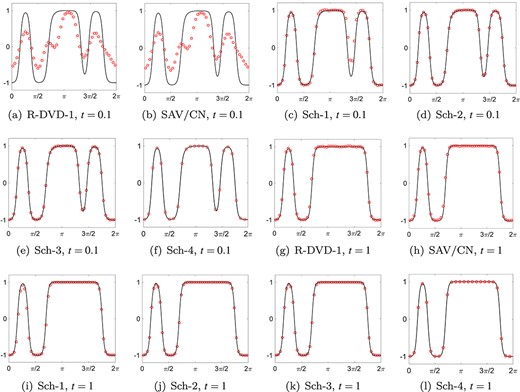
Comparison of the six schemes. The red circles represent solutions obtained by the given schemes with a large time step size |$h=0.01$|, while the black solid lines represent the reference solutions.
Time step size |$h=0.01$| and |$\beta =1$|. Here reference solution is obtained by the SAV/CN scheme with a small time step size |$h=0.0001$|. (a) Modified total free energy |$\hat{\mathcal E}$|. (b) Original total free energy |${\mathcal E}$|.
Appendix B
In this appendix, we introduce mode details on the construction of stage energy stable DVD schemes based on the newly presented framework.
In scheme Sch-2, |$\nu =2$|, |$c_{1}=\frac 1 3$| and |$c_{2}=1$|. The parameters |$ \tilde a_{21}=\frac 12,\, \tilde a_{22}=-\frac 1 2,\, \tilde a_{23}=1$| in (2.8) are determined by using the Taylor expansion method. According to scheme Sch-1, we write the tableau (2.16) as
By set |$\mathbf{z}_{1} = \frac 1 3[(\tilde a_{21}, \, \tilde a_{22},\,\tilde a_{23})^{T}$| |$-(\frac 1 3,\,0,\,\frac 2 3)^{T}]=(\frac 1{18},\,-\frac 1 6,\,\frac 1 9)^{T}$|, we have the scheme Sch-2 as follows
By taking the unit partition vector |$\mathbf{v}$| as |$\mathbf{v}=(\frac 3 2,\,-\frac 1 2,\,\frac 3 2)^{T}$|, the resulting positive semidefinite matrix |$\mathbb{B}$| is
In scheme Sch-3, |$\nu =2$|, |$c_{1}=\frac 1 2$| and |$c_{2}=1$|. The Sch-1 is taken as the low-order approximation of |$ \int _{0}^{h} f(\phi ,\,t)\,{\mathrm{d}}t$|, which is second-order in time. In the Richardson extrapolation, |$p_{0}=2$| and |$\delta = \frac 12$|. The parameters |$ \tilde a_{21},\, \tilde a_{22},\, \tilde a_{23}$| in (2.8) are then set as |$ \tilde a_{21}=\frac 23,\, \tilde a_{22}=-\frac 1 3,\, \tilde a_{23}=\frac 23$|. According to scheme Sch-1, we write the tableau (2.16) as
By set |$\mathbf{z}_{1} = \frac 1 2[(\tilde a_{21}, \, \tilde a_{22},\,\tilde a_{23})^{T}$| |$-(\frac 1 2,\,0,\,\frac 1 2)^{T}]=(\frac 1{12},\,-\frac 1 6,\,\frac 1 {12})^{T}$|, we get the scheme Sch-3 as follows
By taking the unit partition vector |$\mathbf{v}$| as |$\mathbf{v}=(\frac 4 3,\,-\frac 1 3,\,\frac 4 3 )^{T}$|, the resulting positive semidefinite matrix |$\mathbb{B}$| is
In scheme Sch-4, |$\nu =3$|, |$c_{1}=\frac 1 3$|, |$c_{2}=\frac 23$| and |$c_{3}=1$|. The scheme Sch-1 is taken as the low-order approximation of |$ \int _{0}^{h} f(\phi ,\,t)\,{\mathrm{d}}t$|, which is second-order in time. In the Richardson extrapolation, |$p_{0}=2$| and |$\delta = \frac 13$|. The parameters |$ \tilde a_{31},\, \tilde a_{32},\,\cdots ,\, \tilde a_{36}$| in (2.8) are then set as |$ \tilde a_{31}=\frac 38,\, \tilde a_{32}=0,\, \tilde a_{33}=-\frac 18,\, \tilde a_{34}=\frac 38,\, \tilde a_{35}=0,\, \tilde a_{36}=\frac 38$|. According to Sch-1, we write the tableau (2.16) as
Let us denote |$\mathbf{z}=(\tilde a_{31}, \, \tilde a_{32},\,\cdots ,\,\tilde a_{36})^{T}$| |$-(\frac 1 3,\,0,\,0,\,\frac 1 3,\,0,\,\frac 1 3)^{T}$|. By set |$\mathbf{z}_{1} =\frac 1 3 \mathbf{z}$| and |$\mathbf{z}_{2} =\frac 2 3 \mathbf{z}$|, we get the scheme Sch-4 as follows
By taking the unit partition vector |$\mathbf{v}$| as |$\mathbf{v}=(\frac 9 8,\,0,\,0,\,-\frac 1 8,\,0,\,\frac 98 )^{T}$|, the resulting positive semidefinite matrix |$\mathbb{B}$| is
In scheme Sch-5, |$\nu =4$|, |$c_{1}=\frac 1 4$|, |$c_{2}=\frac 12$|, |$c_{3}=\frac 34$| and |$c_{3}=1$|. The Sch-1 is taken as the low-order approximation of |$ \int _{0}^{h} f(\phi ,\,t)\,{\mathrm{d}}t$|, which is second-order in time. In the Richardson extrapolation, |$p_{0}=2$| and |$\delta = \frac 14$|. The parameters |$ \tilde a_{41},\, \tilde a_{42},\,\cdots ,\, \tilde a_{4,10}$| in (2.8) are then set as |$ \tilde a_{41}=\tilde a_{45}=\tilde a_{48}=\tilde a_{4,10}=\frac 4{15},\, \tilde a_{44}=-\frac 1{15},\, \tilde a_{42}= \tilde a_{43}= \tilde a_{46}= \tilde a_{47}= \tilde a_{49}=0$|. According to scheme Sch-1, we write the tableau (2.16) as
Let us denote |$\mathbf{z}=(\tilde a_{41}, \, \tilde a_{42},\,\cdots ,\,\tilde a_{4,10})^{T}$| |$-(\frac 1 4,\,0,\,0,\,0,\,\frac 1 4,\,0,\,0,\,\frac 1 4,\,0,\,\frac 1 4)^{T}$|. By set |$\mathbf{z}_{1} =\frac 1 4 \mathbf{z}$|, |$\mathbf{z}_{2} =\frac 12 \mathbf{z}$| and |$\mathbf{z}_{3} =\frac 34 \mathbf{z}$|, we get the scheme Sch-5 as follows
By taking the unit partition vector |$\mathbf{v}$| as |$\mathbf{v}=(\frac{16} {15},\,0,\,0,\,0,\,\frac{16} {15},\,0,\,0,\,\frac{16} {15}\,0,\,\frac{16} {15})^{T}$|, the resulting positive semidefinite matrix |$\mathbb{B}$| is
As the matrix |$\mathbb{B}$| is symmetric, the lower triangular part of it is not given in here.
In scheme Sch-6, |$\nu =4$|, |$c_{1}=\frac 1 4$|, |$c_{2}=\frac 12$|, |$c_{3}=\frac 34$| and |$c_{3}=1$|. The Sch-3 is taken as the low-order approximation of |$ \int _{0}^{h} f(\phi ,\,t)\,{\mathrm{d}}t$|, which is fourth-order in time. In the Richardson extrapolation, |$p_{0}=4$| and |$\delta = \frac 12$|. The parameters |$ \tilde a_{41},\, \tilde a_{42},\,\cdots ,\, \tilde a_{4,10}$| in (2.8) are then set as |$ \tilde a_{41}=\tilde a_{45}=\tilde a_{48}=\tilde a_{4,10}=\frac{16}{45},\, \tilde a_{44}=\frac 1{45},\, \tilde a_{42}= \tilde a_{49}= -\frac{10}{45},\, \tilde a_{43}= \tilde a_{46}=\tilde a_{47}=0$|. According to scheme Sch-2, we write the tableau (2.16) as
Let us denote |$\hat{\mathbf{z}}=(\tilde a_{41}, \, \tilde a_{42},\,\cdots ,\,\tilde a_{4,10})^{T}$| |$-(\frac 1 3,\,-\frac 1 6,\,0,\,0,\,\frac 1 3,\,0,\,0,\,\frac 1 3,\,-\frac 1 6,\,\frac 1 3)^{T}$| and |$\tilde{\mathbf{z}}=\frac{4}{11}(\frac 1 {12},\,-\frac 1 6,\,0,\,0,$| |$\frac 1 {12},$| |$0,\,0,\,-\frac 1 {12},\,\frac 1 6,\,-\frac 1 {12})^{T}$|. By set |$\mathbf{z}_{1} =\frac 1 4 \left (\hat{\mathbf{z}}+\tilde{\mathbf{z}}\right )$|, |$\mathbf{z}_{2} =\frac 12 \left (\hat{\mathbf{z}}+\tilde{\mathbf{z}}\right )$| and |$\mathbf{z}_{3} =\frac 34 \hat{\mathbf{z}}+\frac 14\tilde{\mathbf{z}}$|, we get the scheme Sch-6 as follows:
By taking the unit partition vector |$\mathbf{v}$| as |$\mathbf{v}=\frac 1 {45}(64,\,-20,\,0,\, 1,\, 64,\,0,\,0, \,64,-20\,\,64)^{T}$|, the resulting positive semidefinite matrix |$\mathbb{B}$| is
As the matrix |$\mathbb{B}$| is symmetric, the lower triangular part of it is not given in here.
