


Abstract
This study addresses the challenge of sustainable, multi-generational energy production by introducing an innovative geothermal-powered system for simultaneous methane, electricity, cooling, and freshwater generation. The configuration integrates a flash-binary geothermal power setup with an Organic Rankine Cycle, dual-effect absorption cooling, multi-stage flash desalination, and a solid oxide electrolyzer cell (SOEC) linked to a Sabatier reactor for CO2 hydrogenation. Financial analysis reveals annual revenue of $63.6 million, with operating expenses of $54.8 million and labor costs of $5.81 million, leading to a 7.3-year return on investment period. Optimized SOEC operation, including higher working temperatures, reduces voltage losses, improving energy efficiency.
Introduction
Researchers are investigating CO2 mitigation solutions because the widespread use of fossil fuels with high carbon content like petroleum, methane, along with carbonaceous rock releases detrimental contaminants like CO2 [1, 2]. These concerns have led to the adoption of sustainable technologies and environmental considerations [3, 4]. A growing worldwide population has increased energy consumption, requiring wise use of oil and gas resources to minimize environmental implications [5, 6]. According to the International Energy Agency (IEA), worldwide energy demand rose 2.1% in 2017, nearly doubling the previous year. Renewable energy sources like geothermal power [7] can be directly harvested or indirectly stored through carbon-intensive fuel manufacture [8, 9] to meet these energy issues [10]. Fuels can be used in transportation, manufacturing, power generation, chemicals, and food. However, high-temperature dissolution of elements and compounds can limit geothermal energy use due to brine and steam corrosion [11, 12]. Geothermal energy and its problems are detailed in Ref. [13]. Along with energy challenges, water scarcity threatens 80% of the world population, emphasizing the need for efficient water and energy use [14]. Despite freshwater resources making up only 3–5% of the earth's water, economic growth and urban population growth have increased industrial and municipal wastewater discharge, polluting aquifers [15, 16]. Climate change has also impacted rainfall patterns and freshwater accessibility [17], impacting hydroelectric energy production [18]. Freshwater and energy shortages are major current issues [19], requiring significant economic considerations in energy system planning and operation due to their high costs. Adopting energy solutions with low environmental impacts and profitable returns can help solve energy and water challenges.
Eco-friendly multi-generation energy systems have been developed due to the simultaneous use of power and related productions such freshwater, H2, and chilling in diverse industries and environmental concerns [20–22]. Recently, renewable-powered combined cooling/heating production (CCHP) systems have gained popularity in residential, commercial, and healthcare contexts [23–25].
Energy storage technologies like power-to-gas (PtG) technology may also reduce energy resource depletion. Electrochemical processes in PtG technology turn electricity into storable gas, connecting electric networks and gas pipelines. PtG often uses extra or renewable electricity to initiate H2, that is utilized in a Sabatier apparatus for the hydrogenation of CO2 to generate CH4. The Sabatier method relies on energy-efficient H2 generation [26, 27]. The SOEC is a popular technique for high-temperature electrolysis of steam [28] and CO2 [29–31], or both [32] to create H2 and CO.
Toro and colleagues [33] examined a Sabatier reaction-based PTG setup to balance source variations and absorb CO2. Pinch, exergy, and thermo-economic evaluations optimized system performance, identified inefficiencies, and assessed methane production costs for PEME and reactor for methane synthesis. Chen and colleagues [34] modelled a combined reactor system that produced CH4 using an SOEC and Fischer–Tropsch procedure and found the ideal operating pressure stands at 3 bar, above that the methane transformation rate does not increase.
If the voltage remains constant, decreasing the electrical charge magnitude throughout the electrolytic process along with raising the force can reduce power usage. Pan et al. [35] investigated gasification and methanation in a PtG system using urban solid refuse gasification with and without an SOEC. A SOEC at 0.3 air ratio increases CO2 conversion to 98% and system efficiency to 67%. In contrast, removing the SOEC and lowering H2 input to methanation produces 44% CO2 conversion and 77% system efficiency. Stempien and colleagues [36] examined the thermal dynamic efficiency of the renewable CH4 generation station with an SOEC together with vessel, focusing on methane synthesis, Sabatier, and WGSR processes. This study also explored how current magnitude, thermal conditions, force per unit area, and initial steam to CO2 rate affect setup execution. Additionally, SOEC-Fischer–Tropsch integration for sustainable hydrocarbon fuel production was examined [37]. Michailos et al. [38] examined four PtG CH4 generation scenarios at a wastewater treatment facility founded on anaerobic fermentation and PEMEC water electrolysis. These scenarios created CH4 from biomethane and H2. The initial case used sediment breakdown and a PEMEC to produce H2, while the second used gasification to replenish H2, reducing electrolyzer capacity. H2 together with CO2 from the pyrolysis procedure was infused into the biogas synthesis vessel at a 1:4 rate in the third scenario, increasing CH4 output without enlarging the electrolyzer but necessitating a larger reactor. The fourth scenario used the same reactor and PEMEC as the first but added a gasification system and integrated gas turbine procedure for electricity. Second scenario has the lowest levelized energy and biomethane production costs at 128 and 135 £/MWh, respectively.
Problem statement:
Current geothermal systems, though valuable for renewable energy generation, typically focus on single-generation electricity production or, at best, basic cogeneration. This limited scope restricts the utilization of geothermal resources, resulting in suboptimal energy conversion rates, decreased operational flexibility, and a relatively high environmental impact. Such systems often do not incorporate efficient carbon management, thereby missing opportunities for CO2 reuse, which could enhance environmental sustainability and economic returns.
A key gap in existing literature is the absence of fully integrated multi-generation geothermal systems that can simultaneously produce methane, electricity, cooling, and freshwater. Multi-functional systems that combine CO2 utilization with renewable energy storage and multiple outputs have the potential to improve both energy efficiency and environmental sustainability. However, most existing technologies lack the infrastructure to support such a complex integration. The need for innovations in system design and optimization is evident, especially in configurations that leverage CO2 conversion processes to generate valuable byproducts like methane.
Our research addresses these gaps by proposing an advanced geothermal-powered multi-generation system. This system combines a flash-binary geothermal setup with an Organic Rankine Cycle, SOECs, a Sabatier reactor, a dual-effect lithium bromide absorption cooling system, and a multi-stage flash desalination unit. The configuration enables simultaneous methane production, CO2 recycling, and efficient energy utilization, resulting in enhanced efficiency and reduced environmental footprint. By addressing these challenges, our study aims to establish a versatile, high-efficiency system that maximizes geothermal resource usage, supports sustainable energy goals, and generates multiple revenue streams, thereby bridging a critical gap in geothermal technology development.
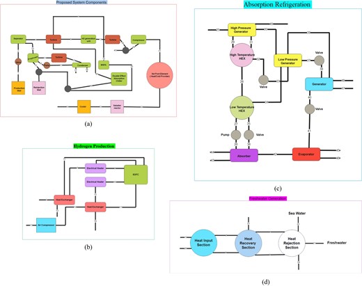
Proposed System Components (a), Hydrogen Production (b), Absorption Refrigeration (c), and Freshwater Generation (d).
An innovative geothermal-powered multi-generation system is introduced in this study to achieve sustainable and clean production. PtG optimizes this multi-generation system to co-generate power, CH4 via the Sabatier process, cooling, and freshwater. The majority of assessments focus primarily on purchase costs [15, 39], while this study accounted for quintupled setup costs and staff expenses [40]. Also included are tax-related cost reductions. Previous studies focused on methane synthesis through the Sabatier reaction, but this study also addressed solid carbon, H2, and CO as key by-products. A thermo-economically optimized binary-flash geothermal energy station, ORC for energy generation, SOEC for H2 production, MSF unit for freshwater, dual-effect lithium bromide absorption cooling cycle for chilling, and Sabatier-based methane synthesis reactor for CH4 production are included in the proposed system. This study's main innovations are listed below.
Introducing a novel geothermal-powered multi-generation system that converts CO2 into CH4 and produces cooling and freshwater.
Conducting a complete economic study, including staffing and installation costs.
Using a cumulative cash flow diagram to assess system financial viability based on SOEC lifetime.
Correctly evaluating the possibility of solid carbon generation during the Sabatier reaction, which could hinder reactor catalyst activity.
Optimizing thermo-economic efficiency with the non-dominant ordering genetic pattern II.
Configuring systems
A flash-binary geothermal energy station, an ORC, a SOEC for hydrogen production, the Multi-Stage Flash (MSF) desalination unit for freshwater generation, a dual-effect lithium bromide absorption cooling process for chilling production, and a Sabatier reaction-based methane synthesis reactor for CH4 production are shown in Figure 1(a). Warm geothermal fluid becomes biphasic flow after passing through a valve. A separator separates the vapor and liquid portions of this mixture. After that, a portion of the ORC's vapor phase (stream 3) is fed into the double-effect absorption refrigeration system's generator to maintain cooling. In the MSF unit, low-pressure vapor from the turbine (stream 19) heats saline water, increasing freshwater output. Figure 1(b) shows how stream 5 vapor reduces hydrogen production unit energy consumption. A hydrogen-rich stream from the electrolyzer's cathode (stream 11) preheats turbine-exit vapor (stream 5) to adjust its molar composition by mixing it with part of the cathode output. An electrical heater changes stream 7's temperature to match stream 8's intake conditions for optimal electrolyzer performance. Electrolyzer electrode's hot output pressurizes as well as preheating the air needed at stream 13 before it is injected into stream 16 following temperature adjustment. In Figure 1(a), SOEC-generated H2 is mixed with CO2 before entering the methanation reactor, where stream 60 adjusts temperature and pressure for the Sabatier reaction. The reaction output (stream 63) is cooled below its dew point to condense water and enrich the gaseous mixture (stream 64) with CH4. Figure 1(c) shows how the extracted steam (stream 25) transfers heat to the Li/Br-water solution, causing refrigerant separation (stream 30) and its movement to the condenser and evaporator for refrigeration. Finally, Figure 1(d) shows the freshwater generation system's heat recovery, rejection, and input portions. Steam from the turbine (stream 19) heats saltwater, enabling freshwater production through flashing stages and distilled water output (stream 21) alongside heated saline water.
Methodology
This study used EES software to simulate the system from thermodynamic and economic viewpoints, followed by MATLAB. The following equation calculates electrolysis energy consumption. In this expression, ΔG represents the change in Gibbs free energy, showing electrical energy consumption. Additionally, TΔS and ΔH reflect theoretical heat values and total power necessary for the procedure [41, 42].
When the electrolyzer voltage is below thermo-neutral, the system functions endothermically, requiring external heat sources. If the thermally neutral potential exceeds the electrolyzer's voltage, surplus heat is created internally, enabling exothermic functioning [43, 44]. Calculating thermo-neutral voltage (Vth) with Eq. (2):
In electrolysis, ΔH, n, and F represent the total heat change, quantity of electrons, and Faraday constant. The solid oxide electrolyzer cell generates H2 and CO at high temperatures by separating steam [28] and CO2 [29–31] or all together [32]. Following is the chemical reaction during steam electrolysis.
The following equation calculates SOEC exothermic heat production [43, 45].
Q, V, and J represent the cell's internal heat, potential difference, and electric flow [46, 47]. The SOEC feed parameters are shown below.
Mass transport in SOEC electrodes
Due to the pressure gradient, mass transfer dominates viscous flow in the porous electrode, which is approximated using the Dusty Gas model [46, 47].
The molar fraction and flux of species i, overall pressure, and effective diffusion coefficients for Knudsen and molecular diffusion between species i and j are represented by yi, Ni, PT, Deff i.k, and Deff J. The universal gas constant and temperature are R and T. Equations (6) and (7) calculate Deff j.k and i.j.
The electrode's porosity and tortuosity are shown by ε and τ, whereas Dj.k and Di.j represent the Knudsen and molecular diffusion coefficients, derived using Eqs. (8) and (9) [48].
Here, r is the average pore radius and M is species j's molecular weight. In Eq. (9), Fuller diffuse volume is V. Eqs. 10 and 11 describe H2 and O2 flow dynamics around the cathode, electrolyte, and anode.
j along with F are electric flow and Faraday's coefficient.
Total electrolyzer potential
difference is calculated using eq. (12) [48].
This formula calculates open-circuit voltage.
E0 is the standard potential, "a" and "c" are electrodes, and TPB is the triphase boundary region. Eqs. (14) and (15) show concentration-induced anode and cathode voltage losses [49]:
Equations 16 and 17 determine electrochemical reaction-related voltage losses at the anode-cathode-electrolyte contact [48].
The equations below calculate the exchange current density j0,
where Ea is the activation energy and parameters A together with B, exponents p, m, along with n vary by electrode material. In Eq. In RohmjSOEC (12), the resistive voltage reduction includes the electrolyte's ionic resistance (Re), the electrodes' electronic resistance, and the overall resistance (Rc) from the electrodes and interconnect [48].
Inlet criteria applied in modelling SOEC.
| Parameter | Value |
|---|---|
| Active area | 73.568 (cm2) |
| Temperature of operation | 760 (°C) |
| Pressure of operation | 95.95 (kPa) |
| Universal gas value | 7.8983 (J mol-1K-1) |
| Faraday constant | 91,660.75 (C mol-1) |
| Anode activation energy | 114 (kJ mol-1) |
| Cathode activation energy | 114 (kJ mol-1) |
| Exchange current density-Cathode | 1.197 ×10¹⁰(mA cm-2) |
| Exchange current density-Anode | 1.9475 × 10⁸ (mA cm-2) |
| Mole fraction-Cathode | 0.95 |
| Mole fraction-Anode | 1.33 |
| Thickness-Cathode | 47.5 (μm) |
| Thickness-Anode | 47.5 (μm) |
| Thickness-Electrolyte | 85.5 (μm) |
| Electric conductivity | 68.4 (Ω -1 cm-1) |
| Nj −8YSZ electric conductivity | 760 (Ω -1 cm-1) |
| Tortuosity | 3.8 |
| Pore radius | 0.95 (μm) |
| Porosity | 0.38 |
The density and electrical conductance of the substance are shown by δ and ρ. Input parameters for electrolyzer cell simulation shown in Table 2. The "Utilization Factor" (UF) controls the molar fractions of H2O and H2 at the cell exit and inlet.
The molar flow rate is represented as ˙ n, with "out" and "in" referring to the electrolyzer's exit and input. According to Ncell, UF is related to cell count. Eq. (24).
Eq. (25) yields Icell, the electrolyzer's current.
Acell and Jcell represent surface area of the cell and charge magnitude. The molar ratios of H2O and H2 at the electrode intake are used to determine a bypass flow (stream 9) between the outlet and inlet.
Multiple phase flash desalination production system
The total mass equilibrium corresponds to eq. (26).
Here, ˙ Mb declares the mass flow ratio of brackish water leaving the heat rejection section's final stage. Equation (27) [19] defines total salt concentration:
where Xf and Xb are the saline concentrations at the last heat rejection stage intake and outflow. Mass current ratio of purified water exiting the potable water generating system is determined using eq. (28).
N represents the quantity of flashing levels, and ˙ Md.i represents the mass current ratio of vapor transformed into liquid throughout every single level. Freshwater production system efficiency is measured by a "Execution Rate," calculated utilizing eq. (29) [50].
The stream rate of hot water from the supplementary heater to the brackish water heating system is represented by ˙ MHW. Equation (30) produces the specific heat transfer area [50]:
Ac and Ab are the thermal energy dissipation and recycle condensers' total areas and the brackish water heater's area. Particular flow ratio of cooling water, a ratio of cooling water to desalinated water flow ratio, is eq. (31) [50]:
Equation (32) calculates the supersaturated vapor mass current rate into the brackish water heating unit.
CR along with DR are chilling and purification ratios. Mass current ratio of supersaturated vapor proceeding into the double-effect absorption refrigeration system's high-pressure generator is also shown in eq.(33).
Sabatier reactor
Chemical changes are shown in Eqs. (34)-(38) [51–54]. The reactor output is determined by minimizing Gibbs free energy for these equilibrium processes.
Inlet criteria utilized in modelling mechanism.
| Parameter | Value |
|---|---|
| Geothermal stream-Flow rate | 47.5 kg/s |
| Geothermal stream-Temperature | 218.5 °C |
| Geothermal stream-Pressure | 2.65 MPa |
| Geothermal stream-Quality | 95 |
| Evaporator-Pinch point | 9.5 °C |
| Evaporator-Temperature | 114 °C |
| Condenser-Temperature | 38 °C |
| Brine heater-Temperature | 110.2 °C |
| Top brine-Temperature | 100.7 °C |
| Intake seawater-Temperature | 23.75 °C |
| Desalination ratio | 94% |
| High-pressure generator-Temperature | 142.5 °C |
| Cooling ratio | 18% |
| High-pressure generator-Temperature | 123.5 °C |
| Low-pressure generator-Temperature | 76 °C |
| Cooling water-Temperature | 24 °C |
| SOEC-Temperature | 760 °C |
| Molar fraction-H2 | 9.5% |
| Molar fraction-Steam | 85% |
| Utilization factor | 96% |
| Methanation-Temperature | 332.5 °C |
The following equations compute rates of CO2 transformation, accompanied by the generation of CH4 and solid carbon.
A "pressure ratio of methanation" (PRM) controls reactor inlet pressure.
P means pressure. To manage the bulk (or molar) flow ratio of CO2 accessing the reactor, an "H2 to CO2 rate" (HCratio) is set.
In this case, ˙ n represents the molar flow rate. Table 3 lists system simulation parameters.
Economic assessment
Energy system development requires economic research and investment return period determination.
This research's total starting cost (TPEC) for equipment is the sum of component expenses. Calculating equipment expenses is explained in [33, 55–57]. Fig. 2 shows expenses beyond acquisition costs as a percentage of TPEC.
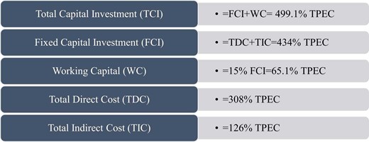
Comprehensive Cost analysis for Establishing an Energy System.
Per Fig. 2, Total Capital Investment (TCI) for an energy system is calculated using the following formula.
And TOC:
This calculation covers raw material and utility expenses (Rm and Ut). Since the system contains no raw materials, raw material costs are insignificant [50]. Similarly, OLC represents operational labour expenses and FCI the total fixed investment. Reference Fig. 2,
Energy and chilling generation systems' operational labour expenses are calculated using Eqs. 48 as well as 49.
H2 and freshwater generation unit operational labour expenses are computed using eq. (50).
where LC is the hourly labor cost and hlabor is the system's workforce's annual working hours (eq. (51)).
The preceding equation defines “plant capacity” as the plant's hourly fuel production in kilos. In addition, np represents the number of processing stages and τ represents the plant's annual operational length. Equation 52 yields gross profit.
S denotes product sales revenue. Equation 53 defines net profit before tax.
D is the depreciation-related investment calculated using Eq. (54).
Calculating net profit after tax:
Inlet economic criteria.
| Parameter | Value |
|---|---|
| Labor expense-Power generation | 0.04275 $/kWh |
| Labor expense-Freshwater generation | 28.139 $/h |
| Labor expense-Cooling generation | 19 $/GJ |
| Labor expense-H2 generation | 28.139 $/h |
| Power price | 0.095 $/kWh |
| Interest rate | 2.1% |
| Extraction expense | 14.478 $/GJ |
| Freshwater price | 2.85 $/m3 |
| Chilled water price | 0.475 $/MJ |
| H2 price | 2.85 $/kg |
| Tax rate | 33.25% |
The tax rate is t. Finally, eq. (56) shows cash flow.
The tax shield on capital depreciation is represented by D×t in the equation above. The investment pays off when the cumulative cash flow is zero. It accounts for component lifespans, among other benefits. Table 4 lists the economic parameters considered in this investigation.
Optimization
Several optimization methods are tested [58], including the non-dominated sorting genetic algorithm II (NSGA II) for two scenarios. This multi-objective optimization seeks thermo-economically optimal system operating conditions. Table 5 lists the main system optimization independent variables. The first scenario prioritizes net power output, while the second prioritizes fuel Lower Heating Value (LHV). The goal is to reduce payback time in both scenarios.
Verification
To verify their accuracy, this study compares Sabatier procedure, MSF system, and dual-effect Li/Br absorption cooling process simulations to literature data under identical operational settings. See Fig. 3(a), Mendoza-Hernandez and colleagues [51] confirm the Sabatier process simulation. Changes within molecular proportions of four entities correlated with temperature at 0.1 Mpa persistent forces per unit area and 2:1 hydrogen to carbon dioxide ratio at the reactor's input are compared. This study's findings match [51], confirming them. This investigation matches Gomri et al. [59] for the absorption refrigeration system, as illustrated in Fig. 3(b), evaluating how low-pressure generator temperature affects system Efficiency Ratio. The results of the 24-stage MSF system are contrasted to those of Desouky and colleagues [50], which used water evaporation at 116 °C as the heat source. Table 6 compares certain heat rejection and recovery stages, while Table 7 compares total results.
The crucial of the suggested mechanism considered as the independent promoting criteria.
| Parameter | Lower bound | Upper bound |
|---|---|---|
| Utilization factor | 48% | 0.95% |
| SOEC-Current density | 2850 A/m2 | 9500 A/m2 |
| Methanation-Pressure | 1.43 bar | 9.5 bar |
| Methanation-Temperature | 142.5 °C | 760 °C |
| SOEC-Temperature | 665 °C | 950 °C |
| Parameter | Lower bound | Upper bound |
|---|---|---|
| Utilization factor | 48% | 0.95% |
| SOEC-Current density | 2850 A/m2 | 9500 A/m2 |
| Methanation-Pressure | 1.43 bar | 9.5 bar |
| Methanation-Temperature | 142.5 °C | 760 °C |
| SOEC-Temperature | 665 °C | 950 °C |

Validation of modelling outlets for the Sabatier procedure (a) and COP of Dual-impact Li/Br absorption refrigeration process (b).
Authenticating the outcomes attained for the present MSF desalination sector on the basis of level statements (a contrast between our research and that of Desouky and colleagues [68].
Authenticating the outcomes attained for the present MSF desalination sector on the basis of level statements (a contrast between our research and that of Desouky and colleagues [68].
Authenticating the outcomes attained for the present desalination cycle on the basis of overall outlets (a contrast between our research and that of Desouky and colleagues [68]).
| Parameter | Value | |
|---|---|---|
| Literature [7] | Current paper | |
| Flow rate-Water (inlet) | 899.65 kg/s | 899.65 kg/s |
| Flow rate-Water (exit) | 868.908 kg/s | 868.775 kg/s |
| Flow rate- Heater vapour (inlet) | 49.894 kg/s | 50.0935 kg/s |
| Flow rate-Recycling | 3215.56 kg/s | 3215.75 kg/s |
| Performance ratio | 6.8495 | 6.821 |
| Flow rate-Specific cooling | 2.2895 | 2.2895 |
| Heat transfer area | 246.62 m2. kg/s | 243.6085 m2. kg/s |
Overall outcomes of the suggested mechanism.
| Parameter | Value |
|---|---|
| Steam turbine | 102.55 kW |
| ORC turbine | 1.36 MW |
| Net power | 526.68 kW |
| LHV | 27.03 MJ/kg |
| Mass flow | 78.32 kg/h |
| CH4 Molar fraction | 50.35% |
| Refrigeration capacity | 3.53 MW |
| COP | 1.14 |
| Power consumption-H2 generation | 0.85 MW |
| Desalination water rate | 39.3 kg/s |
| Area of heat flow | 243.61 m2.s/kg |
| Stream rate of cold water | 2.3 |
| Electrolyzer electricity | 0.8 MW |
| H2 mass flow | 22.3 kg/h |
Using the same baseline circumstances as in [59] to directly compare COP changes versus generator temperature, Fig. 3(b) shows that the dual-effect Li/Br absorption cooling process modeling accuracy is consistent across experiments.
Result and discussion
Summary of results
Table 8 shows the system's performance: 22.9 kg/s gas fuel generation, 28,453 kJ/kg lower heating value, and 53% methane fuel.
This system generates 555.5 kW of electricity, 3716 kW of chilling by lowering feed water temperature from 15 °C to 10 °C, and 42.36 kg/s of freshwater. In particular, the Solid Oxide Electrolyzer Cell (SOEC) produces 6.52 g/s of hydrogen while using 884.47 kW.
An economic assessment
Financial distribution
The financial breakdown is in Fig. 4(a), demonstrating an overall capital investment of 55.2 million USD, with 14% working capital for beginning operations and 87% fixed capital. Direct costs comprise 71% of fixed capital, with equipment installation costs at 28.29 million USD and other direct expenditures at 5.09 million USD. Indirect costs comprise 29% of fixed capital.
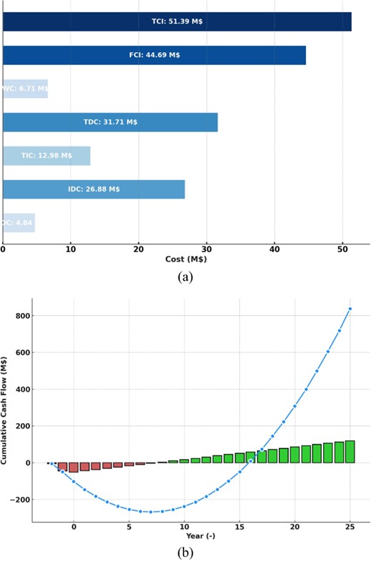
Cost distribution (a) and cumulative cash flow Analysis for the proposed plant (b).
Revenue and operating costs
Table 9 shows operational financials: revenue of 64.2 million USD/year, operating costs of 55.5 million USD/year, and labor costs of 6.06 million USD/year.
The system estimates a 7.32 million USD/year cash flow and a 7.3-year payback to match an SOEC lifespan.
Financial accumulation
Fig. 4(b) shows cumulative money flow. The TCI required over two years and SOEC replacement every three years are considered in Fig. 4(b). The plant breaks even in about seven years, ensuring SOEC financial viability.
Effective thermodynamics
Dynamic methanation
At high methanation temperatures, increasing the pressure ratio boosts CO2 conversion [60]. Higher pressure ratios have less impact at lower temperatures, with the conversion ratio remaining steady below 300 °C. Increasing the usage factor from 1.4 to 2.0 increases methane molecular proportions by 98% and LHV by 35% [61]. Sabatier reaction produces more methane due to the increased hydrogen molar percentage in the intake. Fig. 5(a) examines how a 2 H2 to CO2 ratio affects CO2 conversion and solid carbon and methane production. As solid carbon (C(s)) deactivates catalysts, precise operating conditions are needed to prevent its development. Approximately 600 °C is the minimum permissible temperature to preclude C(s) production under these conditions. Methane output and CO2 conversion ratio also decrease-increase. Fig. 5(b) examines how changing the H2 to CO2 ratio affects the LHV and optimal methanation temperature for zero C(s) production.
The analysis reveals that raising the H2 to CO2 ratio greatly decreases the lowest methane synthesis temperature needed to avoid C(s) generation and boosts fuel LHV. However, it significantly reduces reactor CO2 mass flow. For instance, raising the ratio from 2.0 to 5.0 lowers the lowest temperature by 85%, CO2 flow ratio by 75%, as well as fuel LHV by 417%.
Refrigeration system thermal performance
Fig. 6 shows how the COP of the cooling process affects high- and low-pressure generator temperatures. Initial low-pressure generator temperature increases boost COP until a threshold, after which only negligible gains are seen. However, lower high-pressure generator temperatures correlate with higher COPs, showing that maximizing efficiency requires balancing both high and low generator temperatures.
Organic Rankine cycle
Different ORC working fluid types affect net energy generation as well as system payback period, as shown in Figure 7. Isopropanol gives the system the lowest net power of 388.1 kW and shortest payback period of 7.419 years. The working fluid Isobutane produces the largest net energy production and longest payback period, 121% and 9.2% higher than their minimums. Increased net power requires larger equipment, which increases total capital investment (TCI) and payback duration.
Employment expenses along with revenue of the suggested mechanism.
| Variable | Amount |
|---|---|
| Revenue | 6.099 E7 USD per year |
| Price of the labor | 5.757 E6 USD per year |
| Net price of the operation | 5.2725 E7 USD per year |
| Total benefit | 8.303 E6 USD per year |
| Total benefit (before tax) | 3.8285 E6 USD per year |
| Total benefit (after tax) | 2.489 E6 USD per year |
| Cash flow | 6.954 E6 USD per year |
| Payback period | 6.935 years |
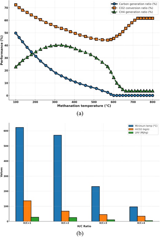
Parameters Influence on Sabatier Reactor Performance.
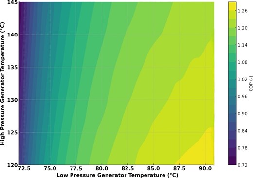
Impact of Generator Temperatures on Refrigeration Cycle COP.
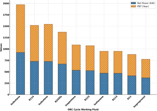
Impact of different working fluid on the net power output and payback period index.
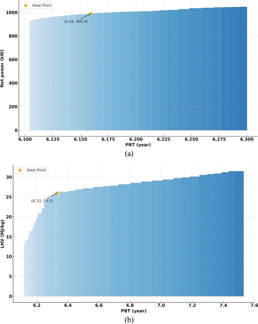
PtG System Optimization: Scenario One Results (a), Scenario Two Results (b).
Optimization
The proposed Power-to-Gas (PtG) system was optimized using the non-dominated sorting genetic algorithm II in MATLAB in two situations, as shown by Pareto fronts. The thermo-economic efficiency peaks everywhere on the Pareto front. The optimal point is elicited by system designers and operators. Initially, an ideal, unattainable point where both objective functions peak is identified. Next, the optimal Pareto front point is chosen as the closest to this ideal. Figures 9(a) and (b) illustrate that this optimal position is labeled point A in the first case and point D in the second. Within the initial case, an increase in net outlet energy from 970 kW to 1102 kW results in a trade-off of 13.6% more power for a 3% longer payback period from 6.1 to 6.3 years. Within the second case, that the lower heating value (LHV) of the produced fuel is prioritized, the LHV ranges from 13.68 to 33 MJ/kg, and the payback period is 6.11 to 7.5 years. A 141% increase in LHV increases the payback period by 23%. Table 1 shows the optimal thermo-economic variables for sites A–F for both scenarios.
In the first scenario, the payback period is 18.7% shorter, net output power is 88% greater, and LHV is 35% lower than baseline conditions at point A. Point B has the biggest net output power increase (98%), and a 19.4% lower payback period. At point D in the second scenario, net output power increases by 95.4% despite a 16.7% longer payback period and a 4.4% lower LHV. At point F, the biggest LHV enhancement is due to raising the utilization factor from 0.5 to 1.0, which only raises net outlet energy by 23.4%.
Limitations and future work
While our proposed geothermal-powered multi-generation system demonstrates significant potential in terms of energy efficiency and environmental sustainability, several limitations warrant attention. First, the system's reliance on specific geothermal conditions, such as temperature and pressure levels, may restrict its applicability to regions with suitable geothermal resources. This limitation highlights the need for future research on adaptable configurations that can operate effectively under a broader range of geothermal conditions. Second, although we have optimized the integration of the Organic Rankine Cycle (ORC), solid oxide electrolyzer cells (SOECs), and Sabatier reactor, additional studies on long-term operational stability and maintenance requirements are essential to ensure consistent performance. Third, the economic analysis, while robust, is based on current market conditions, which may change due to fluctuations in energy prices and regulatory policies. Future studies could incorporate dynamic economic modeling to account for these variables. Lastly, ongoing research on alternative working fluids, optimized catalyst materials for the Sabatier reactor, and advanced CO2 capture techniques could further enhance the system’s efficiency and sustainability.
Conclusions
This thermodynamic and economic research examined a geothermal-powered multi-generational Power-to-Gas (PtG) system. A geothermal energy station, ORC with steam turbine, Multi-Stage Flash desalination system, dual-effect Lithium Bromide absorption cooling process, SOEC, and Sabatier reactor are part of the system. Key findings are below:
i) Revenues are 63.6 million USD, operational expenses are 54.8 million USD, and labor costs are 5.81 million USD. The SOEC's lifespan and 7.32 million USD yearly cash flow yield a 7.3-year payback period. Greater SOEC working temperatures reduce voltage losses, which reduce power consumption, especially at greater current thickness.
ii) Raising SOEC current thickness has a greater effect on cell count than lowering usage factor. Reducing utilization factor to 0.5 reduces cell count by 45%, while raising current thickness from 3000 to 10,000 A/m² at full utilization reduces cell count by 234%. CO2 conversion ratios are high at low methane synthesis temperatures and could be increased by raising the pressure rate at high temperatures, but the effect declines with lower temperatures.
iii) Raising the low-pressure generator's temperature more than the particular point doesn't enhance COP. Lower high-pressure generator temperatures increase COP, hence higher high-pressure generator temperatures require higher low-pressure generator temperatures to produce ideal COP. A maximum net power output of 1102 kW and a minimum of 970 kW were achieved in the first optimization scenario, with payback periods of 6.4 and 6.2 years, respectively. This scenario increased net electricity generation 13.6% but extended the payback period by 3%. The second optimization case maximized fuel LHV while minimizing payback. LHV values ranged from 13.68 to 33 MJ/kg, with payback times of 6.11 to 7.5 years. Increased LHV by 141% increased payback period by 22%.
Acknowledgements
This work is supported by the science and technology foundation of Guizhou Province No. ZK(2024)661. The authors extend their appreciation to the Deanship of Scientific Research at Northern Border University, Arar, KSA for funding this research work through the project number “NBU-FFR-2024-2947-03”.
Author contributions
Tao Hai (Conceptualization [equal], Software [equal], Writing—review & editing [equal]), Abdullah Ali Seger (Funding acquisition [equal], Software [equal], Writing—original draft [equal]), A.S. El-Shafay (Formal analysis [equal], Investigation [equal], Writing—review & editing [equal]), Diwakar Agarwal (Formal analysis [equal], Investigation [equal], Software [equal], Writing—original draft [equal]), Ahmed Jassim Al-Yasiri (Conceptualization [equal], Methodology [equal], Project administration [equal], Writing—original draft [equal]), Husam Rajab (Software [equal], Visualization [equal], Writing—original draft [equal]), Moustafa S. Darweesh (Methodology [equal], Resources [equal], Software [equal], Writing—review & editing [equal]), Lioua Kolsi (Data curation [equal], Software [equal], Visualization [equal], Writing—review & editing [equal]), Chemseddine Maatki (Formal analysis [equal], Investigation [equal], Resources [equal], Writing—review & editing [equal]), and Narinderjit Singh Sawaran Singh (Data curation [equal], Funding acquisition [equal], Validation [equal], Visualization [equal]).
