Dynamic thermal modelling of horizontal ground-source heat pumps Open Access

Abstract

1 INTRODUCTION

A ground-source heat pump is a sustainable technology for heating and cooling of buildings by making use of earth or ground water as the heat source or sink through a heat exchanger. It has lower running costs than a conventional heating and air-conditioning system and is more efficient than an air-source heat pump because of the relatively stable temperature of deep soil, but it is more expensive to install the ground-coupled heat exchanger. A heat exchanger is required to transfer heat between the fluid within the heat exchanger and surrounding soil for a ground-coupled heat pump. The heat exchanger can be installed vertically or horizontally. A horizontally coupled ground-source heat pump makes use of principally solar heat stored in the shallow soil, whereas a vertically coupled ground-source heat pump uses geothermal energy from the earth. A horizontally coupled heat exchanger is cheaper, but requires more land/area to install than a vertical borehole heat exchanger. Besides, the former needs to be longer than the latter for the same heat transfer rate because ambient conditions can have an adverse effect on the short-term performance of a horizontally coupled ground-source heat pump. However, this apparent disadvantage of a horizontally coupled heat pump can in a way become an advantage for long-term operation. Different heat transfer mechanisms between the ambient and ground surface including solar heat gains and heat losses/gains due to long-wave radiation, natural convection and evaporation at different times can alleviate the depletion of heat source/sink of subsurface soil for long-term operation. If more heat is extracted from shallow soil than transferred from deep soil, leading to soil temperature decrease, less heat will be lost to the ambient at times for heat loss and more heat is transferred from the ambient at other times, and vice versa. As a result, a horizontally coupled ground-source heat pump does not suffer performance degradation as much as that could occur to a vertically coupled heat pump if there is a large imbalance in annual heating and cooling loads provided by the system. A horizontal heat exchanger can be straight pipes or slinky coils and a numerical method can be used to predict its performance.

Simulation of horizontally coupled heat exchangers has been carried out by a number of investigators. Mei [1] was one of the first to develop a numerical model based on cylindrical heat transfer equations for predicting temperature distribution in soil buried with horizontal pipes. Tarnawski and Leong [2] developed a computer model for design and simulation of horizontal-coupled ground-source heat pumps, although with emphasis more on the overall system than on the heat exchanger. A more general numerical model was developed by Piechowski [3] for heat and mass transfer through a horizontal-coupled heat pump system with energy storage. Wu et al. [4, 5] and Congedo et al. [6] numerically simulated horizontal slinky heat exchangers for ground-source heat pumps using CFD software FLUENT [7]. Because of the complexity of slinky heat exchanger configurations, the computational domain employed for these simulations was much smaller than a size-independent domain required for accurate simulation of long-term system operation; to be size independent, a computational domain should be sufficiently large such that the transient heat and fluid flow in the area of interests at any time (most likely at the end) of operation would not be influenced by the domain size. Demir et al. [8] calculated heat transfer through a horizontal parallel pipe ground heat exchanger using a numerical method with a uniform mesh size of 0.1 m in each direction and a constant time step of 1800 s. Such large cell and time step sizes might be acceptable for calculation of heat transfer approaching steady state but would not be accurate for simulation of dynamics of heating/cooling processes. Bottarelli and Di Federico [9] compared two types of horizontal heat exchangers—radiator and flat panel—using a three-dimensional finite element code and found that the flat panel type was better than the radiator type according to the expected coefficient of performance.

Less sophisticated horizontal heat exchanger models have been integrated into some building energy simulation tools such as EnergyPlus for faster evaluation. Lee and Strand [10] developed a model implemented in EnergyPlus for simulation of heat transfer through a horizontal earth-to-air heat exchanger. The model took account of variations of air and soil temperatures with time, for example, using an equation similar to Equation (6) to represent the soil temperature at a given location and time, independent of system operation and ignoring interactions between the heat exchanger and soil. Lee [11] attempted to implement in EnergyPlus a two-dimensional numerical model developed by Piechowski [3] for ground heat transfer through horizontally buried pipes. It was shown that implementation of the two-dimensional model with a mesh of 100 radial nodes (0.25 m cell size) would increase computation time by 5–10%. Again the mesh size employed was rather coarse. However, as one of the key features of such a computer program is the speed of computation for design and parametric analysis, a fine mesh (and time step) for more accurate simulation may not be feasible which would lead to a huge increase in computation time—months or years compared with minutes or hours.

Even though simulation of heat transfer through any type of heat exchanger including slinky coils can be performed using a sophisticated commercial software package as demonstrated by some of the investigations mentioned above, such a general purpose software package is not ideal for simulation of the dynamic effects of the fluid in the heat exchanger (i.e. heating/cooling load), daily and seasonal variations in soil and ambient conditions without incurring excessive computing power and cost. An in-house computer program is therefore specifically developed to take account of the dynamic interactions between the soil, heat exchanger, heat transfer fluid (building load) and ambient conditions. This work is concerned with numerical simulation of transient state heat transfer through a horizontally coupled straight heat exchanger for heating operation of ground-source heat pumps using the in-house computer program.

2 METHOD

Simulation of transient heat transfer in soil with possible freezing and thawing is carried out through numerical solution of the following energy conservation equation:

(1)

where ρ, C and k are the density (kg/m³), specific heat (J/kg K) and thermal conductivity (W/m K) of soil, respectively; T the temperature of soil (°C); t the time (s); L the latent heat of fusion of water (J/kg); ρ_i the density of ice (kg/m³); θ_i is the volumetric fraction of ice and q_v the volumetric heat production/dissipation rate (W/m³).

All the thermal and physical properties of a soil mixture can vary with temperature, location and time as well as its constituents such as the moisture content. The density, specific heat and thermal conductivity of a soil mixture are functions of the volumetric composition of three phases—dry solid matter, water and ice:

(2)

(3)

(4)

where subscripts s, w and i represent dry soil, water and ice; f_s or f_i is the average temperature gradient of the constituent (dry soil or ice) to that of water and is given by the following equation [12]:

(5)

where subscript x is either s or i; g_a, g_b and g_c depend on the ratios of the axes of the grains and the sum of them equals to unity. g_j = g_a = g_b = g_c = 1/3 for a sphere, g_j = 0.5 for organic materials and g_j = 0.144 for ice or minerals.

The volumetric moisture content of wet soil is the ratio of the volume of the moisture (water) to the total volume of the soil sample. The sum of water and ice volumes remains the same at any degree of freezing for the given moisture content of soil. For unfrozen soil, the water content is the same as the moisture content whereas the ice content is nil, and for completely frozen soil, the ice content is the moisture content while the water content becomes zero, neglecting the volume change with temperature or phase for any constituent which is implied in the solution below for the computational domain.

The partial differential equation is solved using the control volume method with the following initial and boundary conditions (Figure 1 for a two-dimensional computational domain). The size of the two-dimensional domain is 10 m × 10 m with a non-uniform mesh of 720 000 quadrilateral cells. The edge size of the cells near the heat exchanger is ∼1 mm required for accurate and mesh-independent solution of heat transfer equations, increasing gradually to a maximum of 25 mm at the bottom of the domain. It should be pointed out that the program can be used for three-dimensional models, but this would require a high performance computing facility for the large mesh size (a minimum of 400 million cells for a 50 m long straight heat exchanger and many times more for a slinky heat exchanger) and expensive computation time to achieve the same level of accuracy. Even for a two-dimensional model, it would take ∼12 h for a computer of 3 GHz speed and 3 GB memory to complete a simulation of 24-h intermittent operation for which time steps for calculation need to be small for each day of the operating period (see also the last paragraph of this section), i.e. 3-month continuous computation for simulation of 6-month intermittent operation. For three-dimensional modelling, a computer with an 8 GB memory would only be able to create a mesh for one loop of a slinky heat exchanger in a much smaller computational domain (3 m × 3 m × 4 m) [4].

Figure 1.

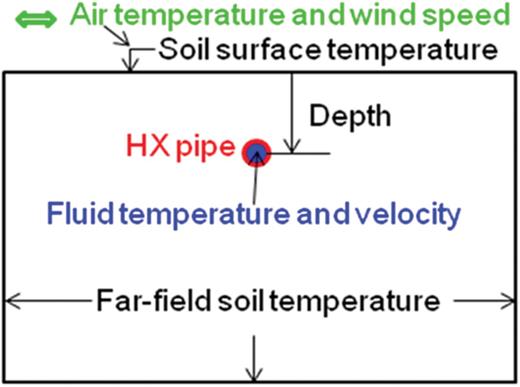
Boundary conditions for simulation of heat transfer through a horizontal-coupled heat exchanger.

Open in new tabDownload slide

The initial soil temperature at time t = t_o and the far-field temperature at any time t (day) and depth Z (m) are given by,

(6)

where T_m is the annual mean temperature of deep soil (°C), T_amp the annual amplitude of surface temperature (°C), t_o the time lag from a starting date to the occurrence of the minimum temperature in a year and D the damping depth (m) of annual fluctuation, ⁠.

Boundary conditions for the soil surface include the ambient air temperature and convective heat transfer coefficient, ignoring the influence of radiation and evaporation heat transfer under vegetation in heating seasons.

The air temperature at any hour of a day in a year is

(7)

where T_min and T_max are the minimum and maximum temperatures (°C) of air in a month and are represented by the following polynomial correlations,

(8)

where m is the month of a year (for example, m = 10 for October) and coefficients a_i and b_i are constants that can be obtained using the meteorological data from a weather station.

The convective heat transfer between the soil surface and ambient air (h_c in W/m² K) includes combined wind and buoyancy effects in the following form,

(9)

The convective heat transfer coefficient due to buoyancy, h_b, is influenced by the soil surface temperature and ambient temperature,

(10)

where k_a is the thermal conductivity of air (W/mK), g the gravitational acceleration (m/s²), ν and α the kinematic viscosity and diffusivity of air (m²/s), respectively, and T_s is the soil surface temperature (°C) from the solution of Equation (1).

The convective heat transfer coefficient due to wind [13]:

(11)

where ρ_a and C_p are the density (kg/m³) and specific heat (J/kg K) of air, respectively, and D_h the heat diffusivity in air (m/s) given by [14]

(12)

with the momentum transfer coefficient D_m (in m/s)

(13)

and Richardson number

(14)

where κ is the von Karman constant, V_z the local wind speed measured at a height of z and is dependent on the measured wind speed at a weather station and the type of terrain, z_o the roughness height of the ground surface which is related to the vegetation height z_veg approximately by z_o = 0.15 z_veg.

The boundary conditions for the internal surface of the heat exchanger pipe during the heat extraction/injection period are similar to those for the soil surface, i.e. the fluid temperature and convective heat transfer coefficient, which could be directly related to the dynamic building heating/cooling load from the time-dependent product of the flow rate, specific heat and temperature change of the fluid in the heat exchanger, which could also be specified simply as a function of ambient air temperature [9] for given specifications and services of a building. The initial physical and thermal properties of soil are determined by the composition and the soil temperature at the starting time of operation using Equations (2)–(6) or from measurement as used in the current work. The initial soil is not frozen for heating operation starting from autumn in the UK.

The heat transfer coefficient for the forced convection between the internal pipe surface and fluid (water with anti-freeze glycol) is [15]:

15

where k_f is the thermal conductivity of the water–glycol mixture (W/m K), d_i the inner diameter of the pipe (m), Re the Reynolds number, Pr the Prandtl number and f the friction factor,

16

Equation (15) is known [16] to be a more accurate correlation for wide ranges of Re and Pr, (2300 < Re < 5 × 10⁶ and 0.5 < Pr < 10⁶), than simpler correlations such as h_f = 0.023 k_f/d_i Re^0.8Pr^1/3 (valid for 10 000 < Re < 1.2 × 10⁵ and 0.7 < Pr < 120). For the base simulation described in the next section, for example, Re ≍ 3180 and Pr ≍37, and the simple correlation would not be suitable for the flow with this magnitude of Reynolds number.

During the switch-off (recovery) period of intermittent operation, zero heat flux is specified as the boundary condition for the pipe surface.

The accuracy of the in-house program was examined by comparing with simulation of heat transfer through a straight pipe of 40 mm external diameter buried 1.2 m below the ground using a commercial program FLUENT [7] which was validated with measurements [4]. Figure 2 shows the predicted specific heat extraction (heat extraction rate per unit length as defined in the next section) using the two programs for a fixed air temperature of 5°C, pipe surface temperature of 1°C and deep soil temperature (=initial soil temperature) of 10°C. It is seen that the results from the two programs agree very well. The differences between them are generally <1% during a period of 30 days.

Figure 2.

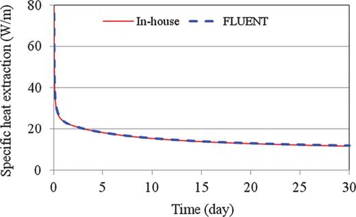
Comparison of the predicted heat extraction rates using commercial and in-house programs.

Open in new tabDownload slide

In order to simulate accurately the transient state heat flow through a horizontally coupled ground heat exchanger, the time step, similar to the mesh size of a computational domain, should be sufficiently small to capture the rapid temperature changes, e.g. at the beginning of continuous operation or switch-on and -off times of intermittent operation. A too large time step from the beginning can lead to under prediction of the pipe surface temperature change and heat extraction rate [17]. The effect of time step is further illustrated in Figure 3 through a comparison of the predicted temperatures of the external pipe surface of the heat exchanger for continuous heating starting from 1 October (same case as for Figure 6) using two different schemes of time steps. One scheme involves the process of using a small time step of 1s or less at the beginning and increasing the time step gradually such that the solution of Equation (1) is independent of the size of time step. Another scheme employs a fixed time step for predicting the heat transfer for the duration of operation. Using a constant large time step would result in a higher predicted pipe temperature than the accurate prediction. For example, with a time step of 600 s, the predicted pipe temperature at the 10th minute is 29% higher than predicted with varying time steps. The relative difference first decreases rapidly with time to 10% in 2.5 days. It then decreases very slowly and reaches a minimum of ∼7.9% at the end of day 22. Afterwards, it increases gradually to 16.3% at the end of November. When the time step is increased to 1200 s, the minimum relative difference increases to 23.5% at the end of day 4 and the relative difference increases more rapidly with time, reaching 63.4% at the end of November. With a smaller time step of 300 s, the relative difference decreases with increasing time; it is 14.4, 2.4, 1 and 0.7% at the 10th minutes, at the end of day 4, end of October and November, respectively.

Figure 3.

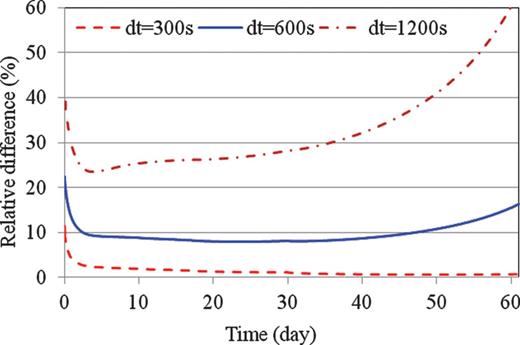
Effect of time step (dt) on the predicted pipe temperature.

Open in new tabDownload slide

3 RESULTS AND DISCUSSION

The method is applied to the simulation of transient state heat transfer through a horizontal-coupled heat exchanger of a ground-source heat pump for continuous and intermittent operation for heating in the UK. The following conditions and assumptions are utilized for the base simulation.

The heat exchanger is made of high density polyethylene with an external diameter of 40 mm, a wall thickness of 3.7 mm and a thermal conductivity of 0.46 W/mK and is installed horizontally at 1.2 m below the ground surface. The fluid in the heat exchanger is a mixture of 65% water and 35% antifreeze and flows in the heat exchanger at a mean velocity of 0.4 m/s (or mass flow rate of 0.35 kg/s) and at a temperature of −1°C. The soil has a density of 1588 kg/m³, specific heat of 1465 J/kgK and thermal conductivity of 1.24 W/mK with a moisture content of 26% according to measurements from an installation site in England [4]. The temperature of deep soil [T_m in Equation (6)] is 10°C and a wind speed at a weather station is assumed at 4 m/s in a rural area. The vegetation height is 0.1 m. Figure 4 shows the predicted daily and seasonal variations in air temperature, heat transfer coefficient between the soil surface and air, and the temperature of undisturbed soil far away from the heat exchanger and at a depth of 1.2 m for the heating season between 1 October and 31 March. The daily air temperature varies by over 5°C. The maximum day time temperature of air is ∼12.5°C at the beginning of heating season and the air temperature drops to near the freezing point during the night of late January. The daily variation of heat transfer coefficient is ∼0.7 W/m²K which results from the variations in both air and soil temperatures, since the wind speed is assumed constant. The trend of seasonal variation of the heat transfer coefficient is opposite to that of air temperature; it reaches the maximum when the seasonal air temperature is at minimum. The temperature of the undisturbed soil at 1.2 m deep is ∼14.3°C, higher than the air temperature, at the beginning of operation and decreases gradually until it reaches the minimum of ∼5°C at the end of February.

Figure 4.

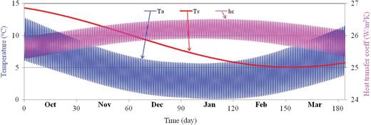
Daily and seasonal variations in air temperature (T_a), convective heat transfer coefficient (h_c) and far-field soil temperature (T_s) at a 1.2 m depth for the heating season (1 October–31 March).

Open in new tabDownload slide

Figure 5 shows the predicted variations with time in soil temperature and heat transfer rate using the heat exchanger for continuous operation starting from 1 October. The time lapse (operating time) is counted from the time when the fluid in the heat exchanger is suddently reduced to the operating temperature from its initial temperature in equilibrium with surrounding soil at the same depth of the heat exchanger rather than from the moment the heat pump is switched on because of the delay of the fluid flow from the heat pump evaporator to different positions along the ground heat exchanger. In the vertical direction, the downward heat tranfer is taken to be positive and upward heat transfer is negative. Heat transfers from warm soil to the cold heat exchanger from all directions. Heat from soil above the heat exchanger is also lost to the cold air during the night time and in the early stages of operation. For example, at the end of day 1, the heat loss from soil to air reaches the mid-distance of the installation depth for the heat exchanger; this is seen from the negative heat flux which decreases from ∼48 W/m² at the soil surface to zero at a depth just over 0.6 m. However, the extent of the heat transfer from soil to air during the night decreases for long-term operation; for example, it is ∼0.17 m at the end of October. During the day time, heat transfers from air to soil and eventually to the heat exchanger even after heating continuously for over 3 months due to the decreasing soil temperature, the overall decreasing rate of which exceeds that of air temperature. The temperature and heat transfer variations during the first day's operation are limited to within 1 m from the heat exchanger. At the end of October, the temperature variation extends over 4 m from the heat exchanger.

Figure 5.

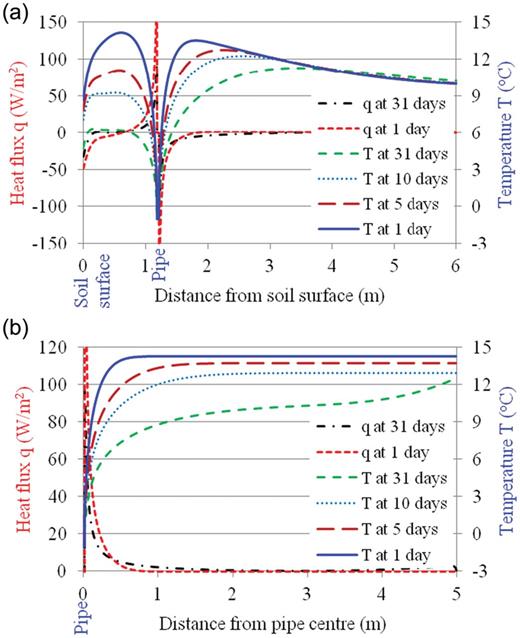
Predicted variations in soil temperature and heat transfer. (a) Vertical direction. (b) Horizontal direction.

Open in new tabDownload slide

The temperature of the heat exchanger (taken as the external surface temperature of the pipe) also varies with time as shown in Figure 6. The variation is very rapid during the first few minutes of operation. It takes ∼30 s for the temperature of the heat exchanger to drop from 14.3°C, the initial equilibrium condition with soil at the installation depth, to 10°C and ∼18 min to drop to 5°C but takes nearly 9 days to 1°C. The temperature would drop to the freezing point after continuous operation for over 2 months.

Figure 6.

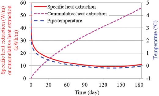
Predicted variations with time of pipe temperature and heat extraction.

Open in new tabDownload slide

The specific heat extraction (rate) is generally used to evaluate the capacity of a ground-coupled heat exchanger and it is defined as the heat transfer rate per unit length of the heat exchanger. The predicted specific heat extraction at start is very high over 100 W/m because of the large temperature difference between the surrounding soil and working fluid. However, it decreases rapidly to <50 W/m within 80 min, 40 W/m in 5h and it drops to <32 W/m before the end of the first day. The specific heat extraction would decrease further for longer periods of operation; it is ∼16, 12 and 10 W/m at the end of October, November and December, respectively (Figure 6). Because of the decreasing heat extraction rate, the cumulative amount of heat extraction would not simply increase linearly with the operating time. The cumulative heat extraction would be close to 16, 26 and 34 kWh/m at the end of October, November and December, respectively. The amount and rate of heat extraction depend on the operating time and installation depth of the heat exchanger as well as other variables including soil properties, ambient conditions, the heat exchanger size and the heating load which is associated with the fluid temperature and/or velocity (or flow rate) in the heat exchanger.

As pointed out in Section 1, one advantage of the horizontal-coupled heat exchanger over the vertical borehole heat exchanger is that the heat in soil extracted during heating seasons could be recharged naturally with solar and ambient heat during the warm seasons. Figure 7 shows that after 6-month continuous operation between October and March, the temperature of soil at the pipe location (pipe temperature) increases with time during the following 6-month recovery period when the system is switched off. The increase in the pipe temperature closely follows the temperature variation of undisturbed soil. The pipe temperature can be fully recovered to the level of temperature (14.3°C) of undisturbed soil at the same depth well within the recovery period for this extremely unbalanced strategy of heat pump operation—long-term continuous heat extraction without artificial heat injection. Much less time (∼2 months) would be needed for the pipe to reach the temperature of deep soil (10°C).

Figure 7.

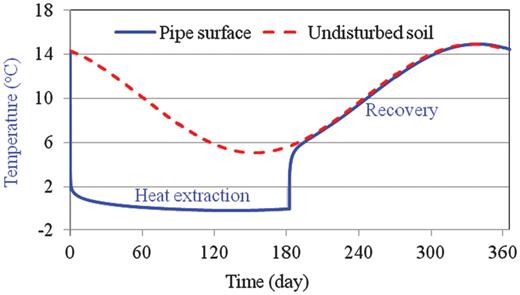
Predicted variation with time of pipe temperature during heat extraction and recovery periods.

Open in new tabDownload slide

3.1 Effect of start time

Because of the seasonal variations of air and soil temperatures, the thermal performance of the heat exchanger would be influenced by the time when the system is switched on. Figure 8 shows the varying heat extraction rate with time for two operation settings—one starts from 1 September and another from 1 October. For the same operation period (duration), the rate is smaller when the operation starts from October than from September (indicated with a negative sign for the difference) because of decreasing air and soil temperature with time until when the soil temperature at the installation depth of the heat exchanger begins to increase early in the following year. The difference is ∼4% at the start of the operation and increases as the operation continues. It reaches a maximum of ∼16.4% at 50 days' operation. The difference then decreases to ∼12% after 3 months' operation. It further decreases to zero after 4 and 2/3 months' operation when the temperature of the soil above the heat exchanger reaches the minimum for the September start but for the October start, the soil temperature has passed this stage [at the end of 5 months at the pipe depth but earlier above the pipe according to Equation (6)] and begun to warm up through the heat transfer from warm air to cold soil in addition to absorption of solar radiation. Consequently, the heat extraction rate for the October start becomes higher than that for the September start afterwards.

Figure 8.

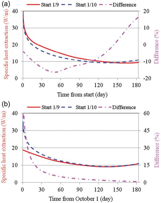
Effect of start time on the predicted specific heat extraction for September and October start. (a) Based on duration of operation. (b) Based on same operating time.

Open in new tabDownload slide

In terms of operating time (defined as the ‘actual’ time when the system is running), the heat extraction rate is higher for operation with a later start date as shown in Figure 8b. For example, on 1 October, the rate for the start time of 1 October is more than twice that for the operation started on 1 September because much of the heat available from the soil surrounding the heat exchanger has already been extracted after the previous 1 month's operation. The difference rapidly decreases to ∼37% on 5 October and 25% on 10 October. It is ∼10% at the end of October and decreases further to ∼5% at the end of November. The difference is negligible at the end of heating season (March the following year).

Similar variation patterns in heat extraction can be observed from start times of October and November (Figure 9). The differences in heat extraction in terms of the operating period are slightly smaller and the maximum difference occurs much earlier than those between September and October start times. For example, the maximum difference between the October and November start times is ∼15% after 20 days' operation compared with over 16% after 50 day's operation for September and October start times. However, in terms of the operating time, the differences are larger for the October and November start times. The difference is ∼42, 27, 11 and 6% on 5, 10, 30 November and 31 December, respectively.

Figure 9.

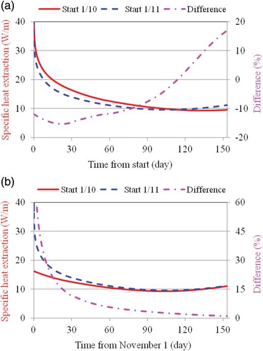
Effect of start time on the predicted specific heat extraction for October and November start. (a) Based on duration of operation. (b) Based on same operating time.

Open in new tabDownload slide

Simulation is also performed for different strategies of intermittent operation from a total of 6–12 h each day. Figure 10 shows two start settings (September and October) for 12-h-on and 12-h-off intermittent operation. It is seen by comparing Figure 10 with Figure 8 that the effect of the operating time for intermittent operation is similar to that for continuous operation both in the trend of variation and the pattern of the difference between two different start times. However, the difference between the two start settings becomes negligible 2–3 months later for intermittent operation than for continuous operation. During the off period, the temperatures of the heat exchanger and soil increase gradually as heat is transferred from the surrounding soil, but the temperature of the heat exchanger could not recover completely to the preceding day's soil temperature in 12 h. As a result, the heat extraction capacity of the heat exchanger would decrease each day. The daily mean specific heat extraction (for September start) decreases from 44 W/m for the first day to 27, 21 and 17 W/m at the end of September, October and November, respectively. It is lower for a later start time of 1 October, decreasing to 23, 18 and 15 W/m at the end of October, November and December, respectively. The daily mean specific heat extraction for the intermittent operation of 12-h running time is up to 30% higher than that for continuous operation as shown in Figure 11 for operation starting from 1 October. In terms of energy transfer, however, continuous operation would provide a larger amount of daily heat extraction than intermittent operation; for the same example, it would be at least 20% larger.

Figure 10.

Effect of start time on the predicted specific heat extraction for intermittent operation starting from September and October. (a) Based on duration of operation. (b) Based on same operating time.

Open in new tabDownload slide

Figure 11.

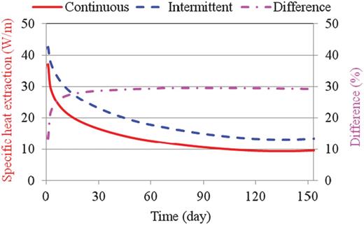
Effect of operating regime on the specific heat extraction.

Open in new tabDownload slide

3.2 Effect of installation depth

The installation depth also influences the thermal performance of the heat exchanger, but the degree of its influence is dependent on the operating time. When operation starts on 1 September, the amount of heat extraction decreases with increasing installation depth of the heat exchanger for the duration of up to 2 months. This is shown in Figure 12a where the heat extraction ratio is the ratio of cumulative heat extraction for a given installation depth to that for a 1.2 m installation depth. The difference is highest at the beginning because of the higher soil temperature at a shallower position and decreases with increasing operating time because the soil temperature decreases at a faster rate at the shallower position. At the beginning of September, compared with the heat exchanger installed 1.2 m deep, the amount of heat extraction is ∼8% and 4% more for the heat exchanger installed 0.6 and 0.9 m deep, respectively, but is 4% and 8% less for the heat exchanger installed 1.5 and 1.8 m deep, respectively. By the end of the month, the differences in the amount of heat extraction decrease to ∼1.3% and 0.5% more for the heat exchanger installed 0.6 and 0.9 m deep, respectively, and 1% and 2.5% less for the heat exchanger installed 1.5 and 1.8 m deep, respectively. The differences diminish at the end of October and the trend of differences would reverse afterwards.

Figure 12.

Effect of installation depth on the cumulative heat extraction. (a) Switch-on time: 1 September. (b) Switch-on time: 1 October.

Open in new tabDownload slide

When the operation is set to start a month later, i.e. 1 October, the higher amount of heat extraction at a shallower position lasts only for 2–5 days. Then, the heat extraction becomes less than if the heat exchanger is installed over the 1.2 m depth. After 20 and 29 days' operation, the heat exchanger installed 1.5 and 1.8 m deep, respectively, would be able to provide more heat than installed at 1.2 m deep. At the end of October, compared with the heat exchanger installed 1.2 m deep, the amount of heat extraction is ∼6% and 3% less for the heat exchanger installed 0.6 and 0.9 m deep, respectively, but is 2% and 2.5% more for the heat exchanger installed 1.5 and 1.8 m deep, respectively. At the end of November, the corresponding differences are 6.6%, 3.3% less and 2.7% and 4.7% more.

Hence, if a horizontally coupled ground-source heat pump is designed for winter heating, its heat exchanger installed at a deeper position would be more efficient. However, for a short period of operation in autumn (or in summer if there is a need for heating, e.g. for hot water or swimming pool), it may be beneficial to install the heat exchanger at a shallow trench.

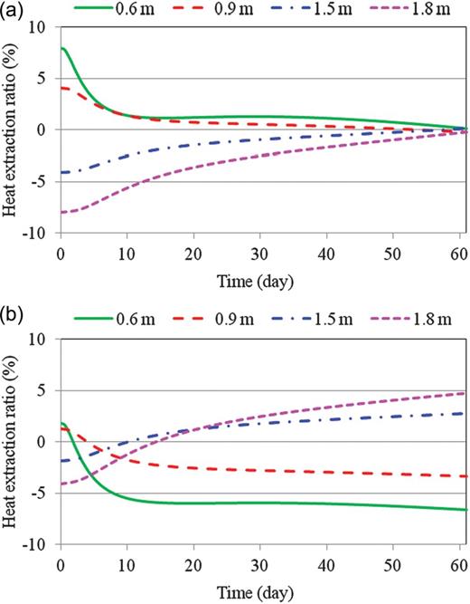
The thermal performance of the heat exchanger would also be influenced by the diurnal ambient temperature variation, but the influence is not obvious from the variation patterns for the specific heat extraction of the heat exchanger installed deeper than 1 m. The influence can however be seen clearly from Figure 13 for the specific heat extraction of the heat exchanger installed 0.6 m below the surface. The specific heat extraction ratio in the figure is the ratio of specific heat extraction for a given installation depth to that for a 1.2 m installation depth. Figure 13a also indicates that the specific heat extraction for the heat exchanger installed at 0.6 m deep is lower than that installed 1.2 m deep from 7 October. Therefore, the larger amount of cumulative heat extraction for the shallower trench results mainly from the higher heat extraction rate in September. This benefit is eroded by the lower heat extraction rate after 7 October and is almost completely negated by the end of the month.

Figure 13.

Effect of installation depth on the specific heat extraction. (a) Switch-on time: 1 September. (b) Switch-on time: 1 October.

Open in new tabDownload slide

3.3 Effect of soil freezing

The temperature of the working fluid increases along the earth heat exchanger of a ground-source heat pump during heat extraction as a result of heat absorption from the soil. The temperature of the exterior surface of the heat exchanger pipe also increases along the fluid flow direction, while the specific heat extraction decreases. Because of the thermal resistance of the pipe, the pipe surface temperature is higher than the fluid temperature in heating operation and so a fluid temperature below 0°C does not necessarily lead to freezing of the soil in contact with the pipe. However, if the fluid temperature is much lower than 0°C, soil close to the pipe could freeze for long-term operation. For example, when the fluid temperature is at −1°C, as mentioned before, the temperature of the external pipe surface would drop to the freezing point after continuous operation over 2 months. If the fluid temperature is reduced further to −3°C, the external pipe surface soil would decrease to the freezing point after continuous operation for 42 h. Such a low fluid temperature could occur even if the system is designed with the operating fluid temperature at the outlet of the heat exchanger above the freezing point of water. For example, when the system is operating with a 3 K temperature increase through the heat exchanger and with an outlet temperature from the heat exchanger approaching 0°C, the fluid near the inlet of the heat exchanger could be −3°C.

When the temperature of soil drops below the freezing point, the freezing model predicts higher soil temperature and heat extraction rate than predicted without the freezing model during and after the freezing process until the heat in the affected soil is ‘depleted’. This results from two sources. One is the release of the heat of fusion from the moisture during freezing. The other is the increased thermal conductivity and diffusivity of soil which are also higher than those of the heat exchanger pipe. For a soil whose thermal conductivity is less than that of ice (=2.2 W/m K), the thermal conductivity increases with the degree of soil freezing [see Equation (4)]. For example, the thermal conductivity increases from 1.2 W/m K for the unfrozen wet soil (26% moisture content) to 1.7 W/m K when it is completely frozen. The extent of soil freezing and its effect on the performance of the heat exchanger depend on the temperature of the fluid, soil properties and duration of heating operation as well as operating regime.

Figure 14a shows that the effect of soil freezing on the pipe surface temperature and heat extraction is not significant when the fluid temperature in the pipe is −1°C, or above. The effect is only observable ∼20 days after the pipe surface temperature reaches the freezing point. The maximum difference is ∼3.4% with the combined effects of heat of fusion and increased conductivity. The effect of the increased conductivity alone is ∼1.7% when freezing of soil in the vicinity of the pipe is complete and the difference between the temperatures predicted with and without the freezing model becomes stable. When the fluid temperature is reduced to −3°C, the influence of soil freezing becomes larger and can be observed sooner in Figure 14b. The temperature of the soil in contact with the pipe would drop below the freezing point after operating for <2 days. The maximum increase in the specific heat extraction resulting from soil freezing reaches 8.6%.

Figure 14.

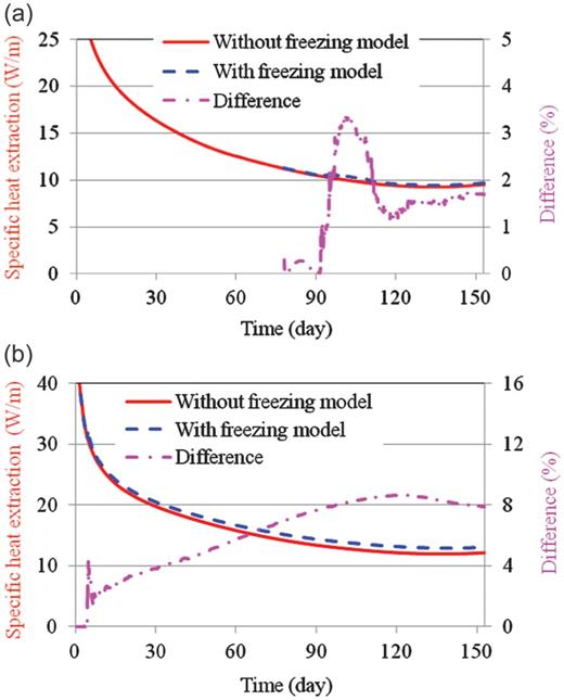
Effect of soil freezing on the specific heat extraction. (a) Fluid temperature of −1°C. (b) Fluid temperature of −3°C.

Open in new tabDownload slide

Whether soil freezing would occur also depends on the soil properties. If the thermal conductivity of soil is higher, the possibility of soil freezing becomes less for a given fluid temperature and velocity. For example, for a soil conductivity of 2 W/mK with the same moisture content (26%), there would be no risk of soil freezing at a pipe depth of 1.2 m with a constant fluid temperature of −1°C during the entire heating period. If, however, the soil thermal conductivity is lower than that of the heat exchanger pipe, the heat extraction rate could become lower soon after soil being frozen. For example, if the thermal conductivity of the wet soil with the same moisture content (26%) was 0.4 W/m K, less than that for the pipe of 0.46 W/m K, the specific heat extraction during freezing would be 2–3% higher, but it would be slightly lower 2h after freezing of the soil in the close vicinity of the pipe. The difference would increase as the heat transfer progresses from the unfrozen soil to the frozen soil (0.55 W/m K conductivity) and then to the pipe because the low soil conductivity become the limiting factor for heat transfer. In practice, only dry soil is likely to have such a low thermal conductivity and hence the effect of freezing would be less than predicted for wet soil.

4 CONCLUSIONS

A computer program has been developed for the simulation of the thermal performance of horizontally coupled heat exchangers for ground-source heat pumps under dynamic climatic, load and soil conditions. The effects of installation depth and operating time of a horizontally coupled heat exchanger have been investigated for heating operation. It has been found that a heat exchanger installed at a shallower depth can provide a larger heat extraction rate at the early stage of heating operation due to the retention of solar heat gains by the soil in summer, whereas the heat exchanger installed at a deeper soil layer is more advantageous after a period of operation, e.g. running continuously for 2 months starting from 1 September. The thermal performance of the heat exchanger is also influenced by the start date of operation. The heat extraction rate for operation with a later start date is lower due to the decreasing soil temperature with increasing time during the heating season but higher at the same heating time because of depletion of heat from the soil during the preceding period. Soil freezing generally enhances heat extraction. This may be beneficial for continuous operation of a heat pump. However, for intermittent operation, frequent freezing and thawing of soil could lead to ‘frost heave’ and this would adversely affect the heat exchanger performance, even though soil is less likely to freeze than under continuous operation for the same soil properties and ambient and working fluid conditions.

The heat extraction/injection capacity of a horizontally coupled heat exchanger decreases with increasing operating time and hence consideration should be given to the design of the horizontal-coupled heat exchanger for heat pumps—a larger/longer heat exchanger is required for longer term and more frequent operation.

The computer program can be used for predicting the dynamic thermal performance of not only horizontal ground source heat pumps but also other types of heating/cooling systems with horizontally buried pipes such as earth–air heat exchangers for ventilation heating/cooling, distribution pipes for district heating/cooling and heat exchangers for heat recovery from wastewater/sewer pipes.

ACKNOWLEDGEMENTS

This research was supported in part by the UK Natural Environment Research Council (Grant NE/F017715/1).

REFERENCES