


Abstract
This study numerically optimizes energy harnessing in vehicle engines using three heat exchanger fin designs: wall to wall, pyramid, and hexagonal. Two thermoelectric generator (TEG) array configurations are compared for electrical power generation. Results show the wall-to-wall fin provides the highest heat transfer, producing 161 W of power from 13 590.53 W of heat. Both TEG configurations generate similar output, with the series offering slightly higher voltage. The flow direction has minimal impact, but increasing the number of heat exchangers boosts efficiency. The total system output reaches 27 763.60 W with a four-parallel exchanger setup and an efficiency of 1.72.
Introduction
The exponential growth of the world population and the rapid progress of industrialization pose a substantial threat to the availability of global energy resources [1–3]. The widespread consumption of energy and the substantial release of carbon dioxide, primarily derived from nonrenewable sources, have led to major global environmental challenges, severely impacting both ecosystems and human society. According to the US Energy Information Administration, global energy consumption is projected to increase by 56% by 2040 compared to 2010 levels [4]. A substantial amount of the energy stored in fossil fuel products is wasted during their production and consumption [5, 6]. It is crucial to find alternative environmentally friendly ways to change the way water and energy resources are used [7–9]. Significant quantities of excess heat generated by industrial facilities and operations are released into the environment, leading to the wastage of energy and the contamination of the surroundings with excessive heat [10]. Hence, the efficient use and retrieval of waste heat holds significant meaning in terms of conserving energy and protecting the environment. Waste heat recovery technologies are widely acknowledged and utilized in various technical applications. Thermoelectric generators (TEGs) are a device that can convert thermal energy into electricity to fulfill the growing demand for electricity from wastage heat sources like automobile emissions, industrial facilities, solar systems, and household heating and cooling systems. The TEG technology is based on many semiconductors that can be utilized to generate electricity [11]. The TEG converts heat, produced by temperature difference, directly into electrical energy by means of the Seebeck effect [12, 13]. TEGs are appropriate for auxiliary generator electrical systems in heavy usage in challenging environments. The use of TEG has many advantages, such as lack of moving parts, maintenance-free operation, small dimensions, the ability to silently generate energy, and the ability to generate electricity in any condition. Different researchers put their efforts to use different wastes or excessive energy in various sources using analytical, numerical, and experimental approaches.
In the field of renewable energy, TEGs are employed in various applications such as thermal management systems, heating and air conditioning, and solar system devices to improve system thermal efficiency and performance by recovering significant thermal losses. He et al. [14] combined experimental and numerical methods to study glass evacuated-tube heat-pipe solar collectors for retrieving waste thermal energy alongside water heating. The prototype consists of a heat-pipe transferring solar heat from the evacuated tube to a thermoelectric module (TEM), which generates electricity from waste heat. The results showed that the thermal and electrical efficiency were about 55% and above 1%, respectively. Karthick et al. [15] suggested a thermal design for a TEG that includes fins connected to a thermal energy storage unit and phase change material (PCM) to store thermal energy. This would allow TEG modules to continuously generate electricity from sunlight, even at night, by using them in both open and closed-circuit states. Results showed power generation during both heating and cooling phases, with net power outputs of 0.39 and 0.31 W, respectively, at a heat flux of 5.5 kW/m2. Cai et al. [16] presented a solar-powered thermoelectric voltage system utilizing a concentrated photovoltaic–TEG (CPV-TEG) and directly using solar power to generate electricity. Their study applied energy balance principles and the first law of thermodynamics to examine the effects of incident solar irradiance, TEGs, and ambient air temperatures on CPV-TEG power generation. Chargui et al. [17] evaluated a novel solar water heating system that incorporates TEGs to convert wasted heat into electricity by utilizing temperature differences in the water. The results showed that the system reduced electricity consumption by 80%, with potential savings up to 90% in warmer climates. Al-Tahaineh and AlEssa [18] conducted numerical analysis to assess the performance of a TEG coupled with a hydronic evacuated tube solar collector heat exchanger for heating in cold regions. TEG is used between hot water circulating through a heat exchanger and the cold surrounding air. The results obtained show that 1.03 W of electricity could be produced when the temperature differences across the TEG and air velocity are 60°C and 0.5 m/s, respectively. Özcan and Deniz [19] investigated the use of TEGs for recovery of waste heat in solar desalination systems to increase water output and efficiency by utilizing condensation latent heat to enhance forced convection evaporation. Energy and exergy analyses have revealed that Conventional Solar Still (CSS)-TEG had higher daily energy (40.34%) and exergy (2.462%) efficiencies compared to CSS (35.55% and 2.403%).
In various sectors such as power generation and manufacturing, where there is significant waste energy, utilizing TEGs for energy conservation is crucial. Pourrahmani et al. [20] simulated the capture of waste heat from proton exchange membrane fuel cells (PEMFCs) by attaching TEGs to the stack walls. Their computational fluid dynamics (CFD) simulation revealed that the PEMFC stack emits 37.7 W of thermal energy, which can be harnessed by TEGs. Zhang et al. [21] introduced a novel combination of a two-stage TEG and a solid oxide fuel cell (SOFC) to capture waste heat from the SOFC for improved performance. The design optimized the number of thermoelectric elements in both stages to maximize power output. Results indicate that this hybrid system (SOFC and TEG) is more efficient than standalone SOFCs. Børset et al. [22] conducted both experimental and mathematical analyses to explore the potential of TEG to recover waste heat from silicon casting. The article implemented a 0.25-m2 TEG utilizing bismuth–tellurium modules in a silicon plant. The results depicted a peak power output of 160 W/m2 with a maximum temperature difference of 100 K across the modules. Ziolkowski et al. [23] employed a finite element model to simulate a TEG positioned between the hot core stream and cool bypass flow at an aircraft turbofan engine’s nozzle, utilizing convection heat transfer to generate electricity for waste heat. The findings demonstrated the TEG could generate 1.65 kW per engine and can reduce operational costs and improve fuel efficiency. Chen et al. [24] developed a new simulation approach that combines CFD with TEGs to recover waste heat from industrial flue gas. Their study evaluated the TEG system’s performance based on factors such as Reynolds number, convection heat transfer coefficient at the cold surface, flue gas inlet temperature, dual TEG, and channel design. Results showed that higher Reynolds numbers, flue gas inlet temperatures, and convection heat transfer coefficients at the cold surface improved TEM performance.
One of other ways that is very globally inclusive between researchers is the waste energy saving achieved by internal combustion engines (ICE). This is because a majority of the energy produced by ICE is transformed into waste thermal energy and released through the exhaust. TEGs are employed to enhance engine efficiency indirectly by utilizing them on the exit of the automobile’s exhaust pipe. Numerous studies have been attempted to investigate the conversion of exhaust heat energy into electricity utilizing various cooling components. Nour Eddine et al. [25] developed a dynamic model in recovering waste heat from automotive engine exhaust, with the electricity generated used to charge a 12 V battery. The model evaluates energy recovery during a specified drive cycle and assesses how system integration impacts TEG performance, including fuel consumption, downstream temperatures, and counter pressure. The results showed maximum power of 42 W generated, with individual modules producing up to 1.5 W. Albatati and Attar [26] introduced an analytical thermal design and validated it experimentally for the TEG system used to recover waste heat from the exhaust of semitruck engines. The settings of the TEG system were tuned in order to attain the highest possible power output. An experiment was performed using a specifically designed setup to confirm the results acquired by analytical methods. The analytical and experimental results were found to have a small deviation, indicating the high accuracy of the effective material properties used in the system. Demir and Dincer [27] presented an innovative way to capture and use passenger vehicle exhaust heat. The exhaust manifold is followed by a heat exchanger. Each heat exchanger pipe has two TEG unit configurations to accommodate exhaust flow rates and temperatures. The intake temperature and exhaust gas mass flow rate directly affect system power capacity. System power output can be increased by 90% by raising exhaust gas mass flow and temperature. Shu et al. [28] presented computational model that simulates a three-dimensional TEG system employed for recovering waste heat from an engine. This study focused on utilizing different factors such as weight increment, backpressure, thinner wall thickness, and moderate inlet dimensions to mitigate these negative impacts in a heat exchanger. There are two configurations of TEMs: a single-TEM segmented structure and a multi-TEM arrangement. The results showed 13.4% increase in maximum output power compared to the original design using single TEM and 78.9 W maximum output power produced by multi-TEM configuration. Ezzitouni et al. [29] focused on the popular engines, which has low energy recovery potential even at high loads. They observed that TEGs can boost engine efficiency without any harm. Despite their low efficiency, thermoelectric materials can improve ICE efficiency globally. Fernández-Yañez et al. [30] examined a light-duty diesel engine (Nissan YD22) numerically and experimentally to use waste heat energy for generating electricity via TEG. The system consists of a diesel oxidation catalyst and a muffler. Pressure and temperature were measured using piezo-resistive pressure sensors and K-type thermocouples. Findings indicated that it is feasible to recover a modest amount of energy during high load and high engine speed conditions, reflecting common driving scenarios. Luo et al. [31] proposed a fluid–thermal–electric multiphysics numerical model to predict TEGs waste heat recovery from automobiles. To accurately simulate operating conditions, the model included geometry, temperature-sensitive material properties, TEM arrangement, and impedance matching. At high vehicle speeds, TEMs on the hot side heat exchanger improve output uniformity. At 120 km/h, the TEG system produces 38.07 W with 1.53% conversion efficiency. Other researchers devoted their efforts mathematically, experimentally, and numerically to work on different aspects of generating electrical power from the waste heat energy of IC engines [32–35].
Some significant works got involved into this work to examine different TEG configurations on the heat recovery. Hsiao et al. [36] focused on optimization of the efficiency of an ICE with TEG system by converting waste heat into electricity. The feasibility of TEG module was investigated in the two areas, the exhaust pipe and radiator. The findings depicted that the module generates a maximum power of 51.13 mW/cm2 at a temperature difference of 290°C. Additionally, the results demonstrate that the TEG module performs better on the exhaust pipe compared to the radiator. Kumar et al. [37] investigated the potential of TEGs to recover waste heat from internal combustion (IC) engines. The study involved detailed experiments on TEG performance under various engine operating conditions, employing a heat exchanger with 18 TEG modules specifically designed for the temperature differential between exhaust gases and engine coolant. Computational simulations were performed to optimize heat exchanger designs, leading to the selection of a rectangular configuration that met spatial and weight constraints. The findings showed that TEG can reduce the size of the alternator or eliminate them in automobiles. Kim et al. [38] carried out a study to evaluate influence of the exhaust gas flow rate of a turbocharged six-cylinder diesel engine under three rotation velocity (1000, 1500, 2000) on the power generated by the TEG. In the study, 40 TEGs were arranged in a 4 |$\times$| 5 pattern, with 20 modules positioned on either the upper and bottom sides of a rectangular exhaust gas channel. The results depicted TEG power output rises with engine load. Luo et al. [39] presented a novel TEG design featuring an inwardly inclined hot-side wall to enhance waste heat recovery from engines. A mathematical model was developed and validated through numerical simulations across five boundary condition scenarios. The findings indicated that increasing the tilt angle improves the Reynolds number and convective heat transfer coefficient, resulting in higher hot-side temperatures. The model showed a maximum temperature error of just 4.24% compared to simulations. The optimal angle for exhaust gas mass flow rates above 37.25 g/s can boosts the TEG’s net power by 5.96%. He et al. [40] conducted a comprehensive mathematical model for evaluation of series-connected thermoelectric components using two different coolant fluids, air and water. In this work, the temperature gradient modeling was utilized to evaluate thermoelectric performance under four cooling strategies to generate electricity from waste heat energy based on direction of flow and the temperature of fluid. Kim et al. [41] worked on experimental exploration for recovery of waste heat with potential of a direct contact TEG (DCTEG) on a diesel engine. The experimental results showed that increasing temperature variations among TEMs, engine loads, and rotation velocities improve DCTEG energy conversion efficiency by 1.0%–2.0%. The DCTEG output power is 12–45 W. Mat Noh et al. [42] used different TEG arrays (series and parallel connections) on an IC engine to test electrical qualities based on the heat absorption and temperature difference between two sides of TEG. The study indicated that sequentially organizing the TEGs increased voltage output, and the series connection produced the most power from ICE waste heat. Raut and Vohra [43] studied a TEG module (TEC1-12715) and waste heat recovery module. One side of the TEG module connected to an aluminum fin and the other is on copper coolant channel. Waste heat recovery module converts and stores energy from Honda GX120 exhaust. The results of this study showed that the pair of TEGs (TEC1–12715) can reach 1.4 V at 3000 rpm. Another device (TEG-27145) outperformed the TEG (TEC1-12715) and generated more voltage. Lan et al. [44] studied a bifunctional TEG for automotive engines that recovers waste heat through the Seebeck effect and heats the engine using the Peltier effect. A four-quadrant operational diagram illustrating cooling, heating, and power generation was developed using a dual-mode TEM model and experimentally validated. The research investigated a 2-L diesel engine and determined that optimal engine oil temperatures (100°C) could solely be attained with the TEG in waste heat recovery and engine warm-up modes.
Some other works considered optimizing approach to improve the efficiency and performance of the exhaust waste heat recovery system. Various geometries of the exhaust channel using fins, ribs, bafflers and other innovative geometries to investigate its effects on heat transfer for the optimization of energy conversion are used. Luo et al. [45] presented a structure-based optimization approach for enhancing the performance of TEGs through the development of a converging heat exchanger design. A multiphysics fluid–thermoelectric coupled field numerical model was employed to conduct comprehensive simulations of the TEG system. The results revealed that the converging design not only generates approximately 5.9% higher output power compared to conventional structures but also reduces backpressure power loss and achieves a more uniform temperature distribution. Additionally, the power increase was found to correlate positively with rising air temperature and negatively with decreasing air mass flow rate. Karana and Sahoo [46] examined the thermohydraulic performance of an exhaust heat exchanger (EHE) with twisted ribs to enhance waste heat recovery in automobiles. Various geometric parameters, including twist ratio (4–8), angle of attack (30°–90°), and pitch ratio (6–10), were experimentally tested over a Reynolds number range of 2300 to 25 000. The results showed a remarkable improvement in heat transfer rate by 164.22% compared to an internally smooth EHE.
A general review of the conducted studies reveals that in all articles, the use of thermoelectric devices as a means to optimize energy utilization has had a significant impact on the performance of the respective systems. Numerous studies have examined various parameters to enhance the performance of power generation systems, such as the number of TEMs, the arrangement of the thermoelectrics, and the positioning of the thermoelectrics on the heat source according to its dimensions and size, among others. According to previous studies, this paper introduces a new numerical approach to harness the properties of TEGs for recovering waste heat energy from exhaust systems, using various array configurations. The study presents innovative models to evaluate how the shape of heat exchangers influences heat transfer optimization and enhances the temperature on the hot side of the TEGs base on the findings of Kim et al. [39]. These insights aim to improve the efficiency of heat transfer between the exhaust and the environment, leading to better electrical generation and utilization. The research investigates three different fin topologies: wall-to-wall fin, pyramid fin, and hexagonal wall-to-wall fin. These designs are analyzed to determine their impact on key performance parameters such as temperature distribution, exhaust flow velocity, and turbulent kinetic energy (TKE). The goal is to identify which design optimizes the thermal conditions for maximum power generation by the TEGs. The study also explores two distinct TEG array configurations, assessing their ability to convert waste heat into electrical energy under varying conditions. Additionally, the effect of exhaust flow direction is examined, comparing counter-flow and co-directional flow setups to determine which yields better performance. For a comprehensive analysis, the system is evaluated with two, three, and four heat exchangers, providing a practical assessment of the best configuration for maximizing heat recovery and electrical output in real-world applications. The objective of this paper is to offer a detailed comparative study of these configurations and heat exchanger designs, ultimately providing guidelines for improving the performance of exhaust waste heat recovery systems.
Methodology
TEG structure
Figure 1 illustrates the schematic of TEG, which converts heat directly into electricity through the Seebeck effect. The module consists of multiple thermocouples made from N-type and P-type semiconductor materials [47]. These thermocouples are electrically connected in series and thermally connected in parallel when paired [48]. When a temperature gradient is applied across the thermocouples, holes in the P-type material and electrons in the N-type material move from the hot side to the cool side, generating a voltage.
Schematic of TEG.
For high-temperature applications, materials such as lead telluride or silicon–germanium are commonly used, while bismuth telluride is preferred for low-temperature environments [49]. The efficiency and performance of TEGs are evaluated based on key factors, including the Seebeck coefficient, electrical conductivity, thermal conductivity, and the dimensionless figure of merit (ZT), which reflects thermoelectric efficiency. A higher ZT value indicates better performance, meaning the material generates a higher voltage per temperature difference, has excellent electrical conductivity, and exhibits low thermal conductivity optimizing overall performance.
Computational model
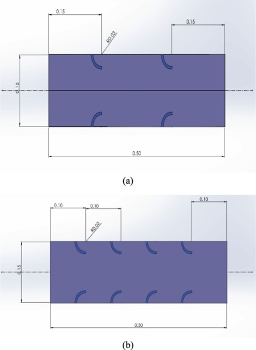
Figures 2 and 3 show different configurations of computational model. In Fig. 2, the system consists of a heat exchanger, coolant channel, and TEG. The models have been designed in SolidWorks 2021 parts and assembly. Figure 2a indicates the model includes a nozzle and diffuser in the inlet and outlet of the heat exchanger in different shapes. The diameter of the inlet nozzle of the heat exchanger is about 60 mm, and the side-to-side length of the hexagonal heat exchanger based on Fig. 2a is around 100 mm. The length of the hexagonal heat exchanger is 20 cm. As illustrated in Fig. 2a, the heat exchanger is hexagonal, with a TEG placed on each side. To study how the structure of the heat exchanger affects TEG performance, three fin-shaped topologies inside the heat exchanger were proposed: (a) wall-to-wall fin, (b) pyramid-shaped fin, and (c) hexagonal wall-to-wall fin. Six rows of TEGs, with three in each row, measuring 56 × 56 × 4.45 mm, are positioned to convert the temperature gradient into electrical energy. The properties of the TEG module are provided in Table 1. For the cooling system, flow is maintained by a pump, with six coolant channels placed on each side of the heat exchanger. The inlet diameter of the cooling channel matches the length and width of the hexagonal heat exchanger. Figure 3 presents a more detailed investigation into the heat energy conversion system, comparing configurations with two, three, and four hexagonal heat exchangers to a single system to find the most efficient design for practical energy conversion applications. Each system in Fig. 3 includes several components: (a) manifolds, (b) muffler, (c) exhaust pipe, and (d) hexagonal heat exchanger. The mass flow rate is divided equally among the heat exchangers, with consistent boundary conditions. Table 2 provides details on the exhaust flow, coolant fluid, and materials used for the cooling channels and heat exchangers.

(a) The heat exchanger. (b) Wall-to-wall fins. (c) Pyramid fin. (d) Hexagonal wall-to-wall fin.
The model with two, three, and four heat exchanger systems.
Governing equations
This study investigates the influence of temperature and exhaust flow rates on the energy generation of TEGs. The researchers employed the Reynolds-averaged Navier–Stokes method along with the realizable |$k-\epsilon$| model, an enhanced version of the classical |$k-\epsilon$| model, chosen for its improved ability to simulate thermal effects with enhanced wall treatment. This model is known for providing a more accurate heat dissipation (|$\epsilon$|) equation and is highly effective in complex flow conditions.
The realizable |$k-\epsilon$| model is known for its superior performance in predicting the behavior of both planar and circular jet flows [50]. The realizable |$k-\epsilon$| model excels at modeling boundary layer behavior, even under challenging conditions such as high adverse pressure gradients, flow separation, rotation, recirculation, and significant streamline curvature [51]. These features make it a powerful tool for optimizing TEG performance across a range of thermal and flow environments. In this study, the flow inside the channel is considered incompressible due to its low velocity, and it is modeled as a three-dimensional, single-phase flow. The exhaust gas flows through the heat exchanger, while a mixture of water and ethylene glycol acts as the coolant in the cooling channel. The flow is transient and highly turbulent, with vortex formations occurring in the EHE.
The continuity, momentum, and energy equations are given in equations (1), (2), and (3):
TEG module
| |$\boldsymbol{\alpha}$| (Seebeck coeffient) | |$\mathbf{478}\ \boldsymbol{\mathrm{\mu}} \mathbf{V}/\mathbf{K}$| |
|---|---|
| Thermal conductivity (W/m K) | 2.18 W/m K |
| Resistance(Ω) | 1.75 Ω |
| Weight (g) | 48 g |
| |$\boldsymbol{\alpha}$| (Seebeck coeffient) | |$\mathbf{478}\ \boldsymbol{\mathrm{\mu}} \mathbf{V}/\mathbf{K}$| |
|---|---|
| Thermal conductivity (W/m K) | 2.18 W/m K |
| Resistance(Ω) | 1.75 Ω |
| Weight (g) | 48 g |
The properties of coolant fluid, exhaust gas, and heat exchanger
| Material | Properties | |
|---|---|---|
| Aluminum | Density (|$\mathrm{k}/{\mathrm{m}}^3$|) | 2719 |
| Specific heat (J/kg K) | 871 | |
| Thermal conductivity (W/m K) | 2.81 | |
| Water–ethylene glycol | Density (|$\mathrm{k}/{\mathrm{m}}^3$|) | 1030.95 |
| Specific heat (J/kg K) | 3551 | |
| Thermal conductivity (W/m K) | 0.414 | |
| Viscosity (|$\mathrm{kg}/\mathrm{ms}$|) | 0.00076 | |
| Exhaust gas | Density (|$\mathrm{k}/{\mathrm{m}}^3$|) | 0.644 |
| Specific heat (J/kg K) | 1043 | |
| Thermal conductivity (W/m K) | 0.044 | |
| Viscosity (|$\mathrm{kg}/\mathrm{ms}$|) | 2.85 |$\times$|10−5 | |
Different parameters are defined in equations (1), (2), and (3), where |$\rho, t,\overrightarrow{v},\mu, c,T$|, and |$\lambda$| represent the density, time, fluid velocity vector, dynamic viscosity, specific heat capacity, temperature, and thermal conductivity of exhaust gas and cooling water, respectively. The governing equation for the realizable |$k-\epsilon$| turbulence model for three-dimensional incompressible turbulence flows can be written as follows:
where
|${x}_j$|: the position vector,
|$\rho$|: the fluid density,
|${u}_j$|: the velocity vector,
|$k$|: the TKE,
ε: the turbulence dissipation,
|${G}_k$|: the generation of turbulence kinetic energy due to mean velocity gradients,
|${G}_b$|: the generation of turbulence kinetic energy due to buoyancy,
|${Y}_m$|: the contribution of fluctuating dilatation in compressible turbulence to the overall dissipation rate,
|${u}_t$|: the turbulent viscosity.
|${C}_2$| and |${C}_{1\epsilon }$|: constants with the value of 1.9 and 1.44.
The values of |${\sigma}_{\epsilon }$| and |${\sigma}_k$| as the turbulent Prandtl number for |$\epsilon$| and |$k$|, respectively, are 1.2 and 1.0. The formula for |${C}_1$| is determined by |$\max \left[0.43,\frac{\eta }{\eta +5}\right],$| where |$\eta$|is defined as |$\frac{k}{\epsilon }$|. The |$S$|is |$\sqrt{2{S}_{ij}{S}_{ij}}$|, showing the rate of strain tensor. The turbulent viscosity |${\mu}_t$| can be defined as |$\rho{C}_{\mu}\frac{k^2}{\epsilon }$|. The eddy viscosity formula is similar to other |$k-\epsilon$| models. However, the difference between this model and the previous two models lies in |${C}_{\mu }$|, which is no longer constant. The |${C}_{\mu }$| is a function of the average strain and rotation rate, which can be defined as follows:
Numerical modeling
Numerical setup
ANSYS Fluent 20 is a computational simulation software that uses the finite volume method to solve equations for continuity, momentum, energy, turbulent dissipation, and TKE. The simulations were run on a system with 10 CPU cores and 32 gigabytes of RAM. The solver’s convergence error for the residuals was set to a minimum of 0.001 for all equations, except for the energy equation, which had a minimum value of 10−6. The SIMPLE algorithm was utilized to couple pressure and velocity using pressure-based correlations. A second-order upwind scheme was selected for calculating momentum, TKE, turbulent dissipation rate, and energy. Table 3 shows the settings used in ANSYS Fluent software to perform this simulation.
Simulation settings of the present study
| parameters | Method | Specification and discretization |
|---|---|---|
| General settings | Pressure based | Transient |
| Turbulence model | |$\mathrm{k}-\mathrm{\varepsilon}$| | Realizable |
| Flow behavior near the wall | Enhanced wall treatment | Thermal effects |
| SIMPLE | ||
| Pressure | PRESTO | |
| Momentum | Second-order upwind | |
| Solution method | TKE | Second-order upwind |
Mesh generation and mesh independent
The computational cost of the research is critical, as it relies on the process of creating a mesh for the model. In order to evaluate the accuracy of the flow simulation of a hexagonal heat exchanger with cooling channels, it is essential to solve the governing equations for several small regions during the mesh construction process. For the meshing part, utilization of structured hexahedral and unstructured tetrahedral meshes for computational purposes was implemented, which were generated using ANSYS meshing. To establish the optimal mesh density for correct results, mesh independence studies gradually improve the mesh and examine the solution changes. The number of meshes and the interval of aspect ratio for each model are listed as follows: (a) for the wall-to-wall fin, the number of meshes is set to 800 000, with an aspect ratio between 1.17 and 18.86; (b) for the pyramid-shaped fin, meshes are 600 000, with an aspect ratio of 1.25 to 16.13; and (c) for the hexagonal wall-to-wall fin, the number of meshes was set to 800 000, with an aspect ratio of 1.25 to 17.79 (Fig. 4).
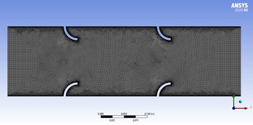
The mesh distribution for each model case.

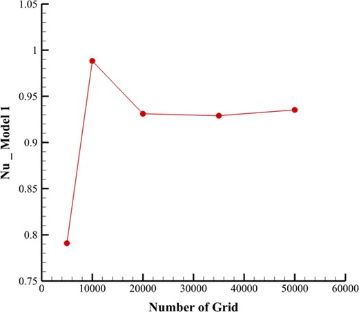
The mesh independent for simulation.
Mesh independence was achieved in the simulation to ensure accurate results. The temperature results for the first row of TEG at the maximum mass flow rate were presented for the wall-to-wall fin model. Eventually, the mesh generation remained consistent, confirming the independence of the mesh from further refinement (Fig. 5).
Numerical initial conditions
For implementing the simulation of the EHE, six cooling channels, and three TEGs on each side of the hexagonal shape of the EHE, as the initial condition for solving the equation of each node were considered. Based on it, determining the domain of the solver for co-flow/counter-flow and the system of the heat exchanger are considered. Table 4 depicts the mass flow rate and temperature of the inlet exhaust of the heat exchanger in four various situations based on Ref [39]. The simulation uses the velocity inlet and pressure outlet to determine the boundary condition of the numerical model. Table 5 determines the initial condition of each cooling channel. The number of cooling channels is 6, with a constant mass flow rate for all the various cases.
The initial condition of different models
| Model name | Air manifold area (m2) | Inlet air mass flow rate (kg/s) | Inlet air velocity (m/s) | Inlet air temperature (°C) |
|---|---|---|---|---|
| Model 1—wall-to-wall fin | 0.002827 | 0.0223 | 12.24878 | 174.75 |
| Model 2—pyramid fin | ||||
| Model 3—hexagonal fin | ||||
| Model 1—wall-to-wall fin | 0.0263 | 14.44588 | 236.64 | |
| Model 2—pyramid fin | ||||
| Model 3—hexagonal fin | ||||
| Model 1—wall-to-wall fin | 0.0301 | 16.53312 | 289.35 | |
| Model 2—pyramid fin | ||||
| Model 3—hexagonal fin | ||||
| Model 1—wall-to-wall fin | 0.0344 | 18.89499 | 334.85 | |
| Model 2—pyramid fin | ||||
| Model 3—hexagonal fin |
The initial condition of cooling channels for different models
| Number of cooling channel | Area of each water channel (m2) | Inlet water mass flow rate in each channel (kg/s) | Inlet water velocity in each channel (m/s) | Inlet water temperature (°C) |
|---|---|---|---|---|
| 6 | 0.00138 | 0.02222 | 16.10144928 | 20 |
| Number of cooling channel | Area of each water channel (m2) | Inlet water mass flow rate in each channel (kg/s) | Inlet water velocity in each channel (m/s) | Inlet water temperature (°C) |
|---|---|---|---|---|
| 6 | 0.00138 | 0.02222 | 16.10144928 | 20 |
The initial conditions for TEG systems for two, three, and four parallel EHEs and the counterflow system are determined in Tables 6 and 7.
The initial conditions for system of TEGs
| The best model | Air manifold area (m2) | Inlet air mass flow rate (kg/s) | Inlet air velocity (m/s) | Inlet air temperature (°C) |
|---|---|---|---|---|
| Two parallel EHEs | 0.00282 | 0.0172 | 9.44749 | 334.85 |
| Three parallel EHEs | 0.00282 | 0.0115 | 6.31664 | 334.85 |
| Four parallel EHEs | 0.00282 | 0.0086 | 4.72374 | 334.85 |
The initial conditions for different cooling channels for systems of TEGs
| The models | Number of cooling channel | Water channel area (m2) | Inlet water mass flow rate in each channel (kg/s) | Inlet water velocity in each channel (m/s) | Inlet water temperature (°C) |
|---|---|---|---|---|---|
| Counter-flow system | 6 | 0.00138 | 0.02222 | 16.10144928 | 20 |
| Two parallel EHEs | 12 | 0.00138 | 0.01111 | 8.050724638 | 20 |
| Three parallel EHEs | 18 | 0.00138 | 0.007407 | 5.367391304 | 20 |
| Four parallel EHEs | 24 | 0.00138 | 0.005556 | 4.026086957 | 20 |
Validation and analysis
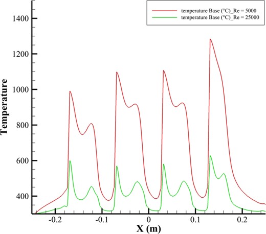
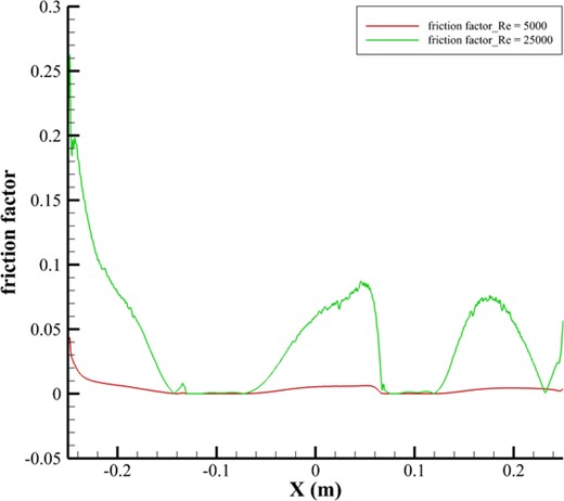
To ensure accuracy and select the most reliable method for precise results, a validation test was conducted based on the reference article [26]. This test examined how changes in fin thickness affected the overall heat transfer rate within the system. Three different turbulence models were tested for validation: the SST |$k-\omega$|, realizable |$k-\epsilon$|, and RNG |$k-\epsilon$| models. In Fig. 6, results showed that the realizable |$k-\epsilon$| model provided the most accurate representation of heat transfer characteristics and system geometry, with a relative error of only about 2% in most cases. This demonstrated its superior reliability compared to the other models. Based on these findings, the realizable |$k-\epsilon$| model was chosen for all subsequent simulations in this study, ensuring consistent and highly accurate results in line with the reference article’s data.
Energy calculation procedure
An investigation has been conducted based on the first law of thermodynamics states that an ICE converts some of its fuel combustion energy into mechanical power and the most of them transfers as heat to the coolant and releases the rest through exhaust gases. As exhaust gas enters the atmosphere through the exhaust pipe, some energy is lost through the pipe walls. Using a TEG may recover some of this lost energy and enhance the supply of more efficient electricity. Transformation of thermal energy into electrical energy was conducted by studying different configurations of arrays of TEG connectors. Two system of arrays is proposed that are shown in Fig. 7a. The TEGs are positioned in a series array configuration surrounding the heat exchanger, that are subsequently grouped into three parallel rows. Figure 7b illustrates the configuration of TEMs, with a series connection on each surface of the heat exchanger and a parallel connection of rows on each side. The method for calculating series and parallel configurations of TEGs follows the same principles as calculating resistances in electrical circuits. In a series configuration, the individual voltages generated by each TEG module are summed, resulting in a higher total voltage. At the same time, the total resistance is calculated by adding the resistances of all the modules and the load linearly. In a parallel configuration, the currents produced by each module are combined, just like how currents sum in a parallel resistance circuit. However, the calculation for total resistance is different: the reciprocal of the total resistance is the sum of the reciprocals of the individual module resistances and the load.
Validation of heat transfer rate according to fin thickness.
The schematic of two configurations of a group of TEGs around the heat exchanger. (a) The series configuration. (b) The parallel configuration.
For calculating the power output from the TEG modules, the temperature of two sides of the TEG is important. Energy conversion is based on various electrical parameters, such as load electrical resistance, electrical current, and the generation of potential difference. According to the following formula, |${Q}_h$| and |${Q}_c$| can be calculated:
In equations (7) and (8), |$I,T,\alpha, \sigma$|, and |$k$| are current, temperature, seebeck coefficient, electrical conductivity, and thermal conductivity, respectively. The current of the TEG can be derived as follows:
|$ {R}_L $| is related to load resistance and |$ {R}_T $| is the internal resistance. The output power can be derived by calculating the difference between |$ {Q}_h $| and |$ {Q}_c $|:
Attaining the maximum output power can be calculated when the load resistance (|${R}_L$|) is equivalent to the actual TEG resistance (|${R}_L={R}_T=R$|). The maximum electric output power can be found as follows:
The voltage can be derived by the following equation:
Results and discussion
Based on Fig. 8, the temperature variations of three rows of the TEGs module around the heat exchanger are compared. Temperature changes are based on exhaust flow changes. According to increases in the flow rate and speed of exhaust movement, the transferred heat increases, and as a result, the surface temperature of the heat exchanger increases. It can be seen that the wall-to-wall model has almost the same temperature changes as the hexagonal wall-to-wall fin model, and the addition of hexagonal fins to the wall-to-wall model has significant changes in the amount of heat transfer and has not caused an increase in surface temperature. By comparing Fig. 8a with Fig. 8b and c, it can be understood that the temperature of the exhaust at the beginning of the channel is high and the heat transfer rate is also higher, as a result of the increase in the surface temperature around the heat exchanger. The lowest temperature in mass flow rate is 0.022 |${\mathrm{m}}^3/\mathrm{s}$| (Fig. 8c). The highest temperature corresponding to the maximum mass flow rate (0.0344 |${\mathrm{m}}^3/\mathrm{s}$|), the highest temperature is related to (Fig. 8a).
The temperature on the heat exchanger is measured at the following points: (a) first row of TEGs at the inlet, (b) second row of TEGs in the middle, and (c) third row of TEGs at the outlet.
Investigating the load resistance of different configurations of TEGs
Figure 9 illustrates that the electrical resistance of the TEM circuit increases as the flow of hot exhaust gas intensifies. This trend can be attributed to enhanced heat transfer, elevated temperatures on the TEG’s hot side, and alterations in the thermoelectric materials’ electrical properties. Comparing Fig. 9a and b reveals that shifting the module arrangement from series to parallel configuration results in a reduction of the system’s electrical resistance. The range of electrical resistance variations in series and parallel modes spans approximately 3.45 to 4.05 Ω and 0.86 to 1.02 Ω, respectively. In the wall-to-wall model, the resistance due to loading is marginally higher than in the hexagonal wall-to-wall case, with only slight differences between their values. The pyramidal fin configuration, however, generates a lower temperature on the TEG’s hot side due to its structural characteristics, consequently diminishing the electrical resistance.
The load resistance of two TEG configurations. (a) The series configuration. (b) The parallel configuration.
Investigation of the current of different configurations of TEGs
According to equation (9), the current in the TEGs array is dependent on the temperature changes and the value of the internal resistance of each TEM and the load resistance of the circuit. According to Fig. 10, the TEGs are placed in the form of series configuration. The current changes in the entire circuit for the wall-to-wall fin model and the hexagonal model are almost the same, but for the pyramid fin model, it has lower current than the other ones because of lower temperature changes. As it is known, the current depends on the temperature changes: the higher the temperature, the more current produced in the circuit. By comparing Fig. 10a and b, it can be understood that in the state of Fig. 10a, less current is produced than Fig. 10b because the overall resistance is higher in series configuration than the parallel configuration.
The current of two TEG configurations. (a) The series configuration. (b) The parallel configuration.
Investigation of the voltage of different configurations of TEGs
In Fig. 11, variations in voltage are depicted as a function of changes in the mass flow rate of hot exhaust gas in both series and parallel system modes. These variations are influenced by the generated current and the load resistance in the circuit. As shown in previous figures, both the current and resistance increase as the temperature of the hot surface of the modules rises. Figure 11a, which represents the series mode, generates a higher voltage compared to Fig. 11b, which represents the parallel mode. This is because the load resistance in the series mode circuit is higher, having a more significant impact than the current on the voltage generation. In series mode, voltage variations range from 8.5 to 26 V, while in parallel mode, they range from 4.5 to 13 V.
The voltage output of two TEG configurations: (a) The series configuration. (b) The parallel configuration.
Investigation of the generation power of different configurations of TEGs
According to equation 10, Fig. 12 illustrates the system’s output power generation in both series and parallel modes based on the mass flow rate of hot gas flow. The output power of the system is enhanced by increasing the mass flow rate of the exhaust gas, which raises the temperature of the modules’ hot surface, as observed with other components studied. Both wall-to-wall fin and hexagonal wall-to-wall fin exhibit similar trends in Fig. 12a and b. Overall, comparing Figs. 12a and b indicates that the output power in series and parallel modes is nearly identical. The highest output power is associated with the wall-to-wall vanes model at the maximum mass flow rate (0.0344 m3/s), with both Fig. 12a and b showing identical values of 161 W.
The system output power generation of two TEG configurations: (a) The series configuration. (b) The parallel configuration.
Velocity contours
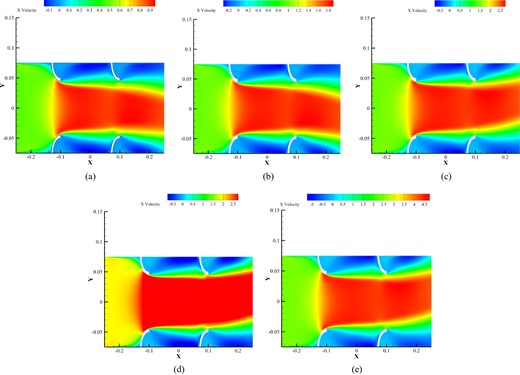
Based on the velocity contour shown in Fig. 13, which takes into account the channel’s geometry, the exhaust’s mass flow rate passes through the edges and makes more contact with the hexagonal side surface. Because of this, the velocity increases in the side areas, resulting in more efficient heat transfer to the surrounding surfaces and a higher temperature on the TEG modules. The EHE’s front view clearly demonstrates this. Additionally, the inlet diameter and geometry of the cooling channels increase the flow velocity in the middle area, facilitating effective heat transfer to the cold surface of the TEG module. Also, the backflow and eddies created in the space around these channels will increase the turbulence of the flow, and this will increase the heat transfer rate. According to the contours in Fig. 13a to d, an increase in the mass flow rate of exhaust in the channel from 0.0223 to 0.0344 kg/s results in a maximum fluid flow velocity of 20 to 27 m/s and a minimum velocity of approximately −10 to −8 m/s. These backflows have decreased in velocity due to increased fluid momentum. The maximum backflow at the end of the heat exchanger makes the pressure decrease severely. The contours reveal that the shape of the nozzle at the heat exchanger’s inlet causes a separation of flow and backflow, which intensifies as the inlet mass flow rate increases. This issue can be seen in the side view of the velocity contour for all geometries.

Velocity contours at different mass flow rates: (a) 0.0223, (b) 0.0263, (c) 0.0301, and (d) 0.0344 for the wall-to-wall fin model.
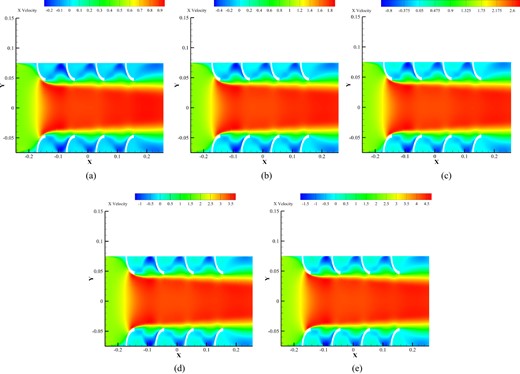
Figure 14 presents the velocity contour of the exhaust flow at the maximum mass flow rate for the second and third geometries. As can be seen, the maximum and minimum velocity of the exhaust flow are approximately equal to 30 and −5 m/s, respectively. This shows that these two geometries have a higher velocity than the first geometry. However, this maximum velocity did not occur at the surrounding or heat exchanger and near the hot surfaces of the TEG module; it mainly happens at the center of the heat exchanger, which has a negative effect on the heat transfer to the TEGs located on each side of the heat exchanger. The majority of the fluid passes through the channel and exits without any heat transfer. That being said, the first geometry has better performance and efficiency than the third geometry, and the third geometry has better heat transfer than the second geometry.
Velocity contours of different models: (a) wall-to-wall fin, (b) pyramid fin, and (c) hexagonal wall-to-wall fin.
Turbulent kinetic contours
Figure 15 shows the side view turbulence kinetic energy profile of combustion products flowing inside the wall-to-wall fin heat exchanger at different mass flow rates. Increasing the fluid velocity causes flow disruption and increases turbulence maximum kinetic energy from 10 to 25 m2/s2 from a to c. Figure 15 shows that flow turbulence and kinetic energy have increased in the boundary layer generated by fluid contact with the solid wall. Because the flow separates from the wall as the fluid enters the diffuser, the vorticity increases and turbulence grows, resulting in a TKE value of roughly 10 m2/s2 at the maximum flow rate.
TKE contours at different mass flow rates: (a) 0.0223, (b) 0.0263, (c) 0.0301, and (d) 0.0344 of wall-to-wall fin model.
Figures 16 shows a comparison between wall-to-wall fin and two other geometries. As in the previous study, contours show that flow separation in the diffuser area increases turbulence kinetic energy. Figure 16b and c has maximum TKE of 19.5 and 18 m2/s2. This factor demonstrates that the first geometry had more maximum turbulence than the other two, which explains its better performance. As mentioned, flow turbulence increases heat transmission between heat exchanger wall s and fluid.
TKE contours of different models: (a) wall-to-wall fin, (b) pyramid fin, and (c) hexagonal wall-to-wall fin.
Temperature contours
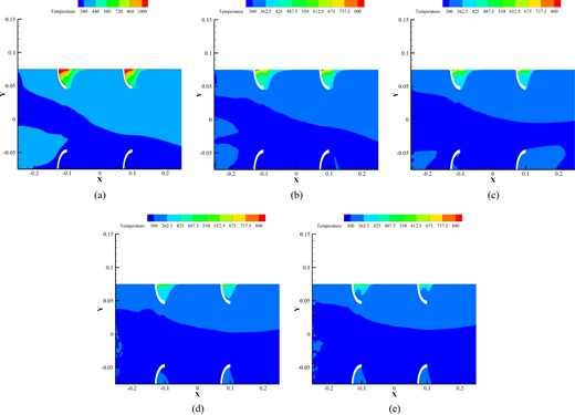
Based on the temperature contours shown in Fig. 17a to d, an increase in the flow rate of the exhaust entering the heat exchanger is correlated with a rise in its temperature. This is because a higher mass flow rate of exhaust signifies increased fuel consumption and a higher rotation speed of the combustion engine, which in turn elevates the combustion temperature. Consequently, this rise in temperature, combined with the increased velocity of the exhaust flow, enhances the heat transfer rate to the fins inside the channel. These fins then transfer the heat to the TEGs located around the heat exchanger. As a result, the temperature on the hot side of the TEG module increases. Because of TEGs’ physical characteristics, the temperature increase on the hot side of the module is significantly higher than on the cold side. This leads to a greater temperature difference between the two sides of the TEG module, thereby boosting power generation due to the temperature gradient.
Temperature contours at different mass flow rates: (a) 0.0223, (b) 0.0263, (c) 0.0301, and (d) 0.0344 of wall-to-wall fin model.
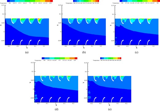
Figure 18 illustrates the temperature contour of the second and third geometries at the maximum flow rate and inlet temperature. According to Fig. 18a to c, the maximum and minimum temperatures in the first, second, and third geometries are roughly equivalent. In the geometries related to the second and third models, more high-temperature exhaust flows through the middle of the channel. This causes most of the exhaust to exit the channel with minimal heat transfer to the base of the fins and TEG. Conversely, in the first geometry, most of the hot exhaust mass flow passes by the base of the fins, effectively transferring heat to the wall. Additionally, the contours indicate that the highest temperature on the hot surface of the TEG modules in all geometries occurs in the first six rows around the heat exchanger inlet. As the flow progresses through the channel and the exhaust temperature decreases, transferring heat to the fins inside the heat exchanger, the heat transfer rate of the fluid diminishes, and the temperature of the hot side of the pyramid fin and hexagonal wall-to-wall configurations decreases accordingly.
Temperature contours of different models: (a) wall-to-wall fin, (b) pyramid fin, and (c) hexagonal wall-to-wall fin.
Comparison of counter-flow and co-flow
According to the results, the wall-to-wall fin geometry has better thermal performance than the other two models. Other investigations have been implemented based on the efficiency of this model at maximum mass flow rate. Figure 19 shows the exhaust temperature contour, TEG, at the maximum mass flow rate for the counter-flow of the exhaust and the coolant. Investigations show that the amount of heat flux transferred from TEG modules is approximately the same amount in both co-flow and counter-flow, which proves that these two states do not represent a significant difference in the performance of the heat exchanger system.
Temperature contour of counter-flow at maximum mass flow rate.
Comparison of different systems of heat exchanger
According to Fig. 20, the temperature contours for each of the two, three, and four EHEs for the wall-to-wall fin model are shown. As it is known, by dividing the exhaust input into several channels, the flow velocity in each channel is reduced. The amount of heat transfer in each channel is lower than the single heat exchanger because the momentum of the exhaust is reduced, and as a result of the reduction of the velocity of the exhaust near the side wall of the heat exchanger, the heat transfer between the exhaust and the wall-to-wall fin is reduced. However, in general, the use of several parallel systems has advantages over one system. Table 8 shows the efficiency of different TEG array configurations at the maximum exhaust inlet mass flow rate for all the investigated models in this research. According to Table 8, wall-to-wall fin geometry has better thermal performance than the other two geometries. For an accurate comparison between the number of systems for a practical usage, the overall thermal performance of the setup is improving by increasing the number of heat exchanger systems, and the model includes four parallel systems. The wall-to-wall fin geometry has the better efficiency for recovery of exhaust waste heat energy.
The schematic of two, three, and four heat exchanger system and the temperature contours.
Practical applications and limitations
The discussed system of using TEGs to recover heat from hot exhaust gases offers several promising real-world applications. In the automotive industry, TEGs can be integrated into vehicles to convert waste heat from exhaust gases into electrical power, which can power auxiliary systems, reduce alternator loads, and improve fuel efficiency. This is especially beneficial for hybrid and electric vehicles, where TEGs could enhance battery charging, extend driving range, and reduce fuel consumption. In industrial settings, many processes generate significant waste heat, and TEG systems can capture and convert this heat into electricity, improving energy efficiency and reducing operational costs. This application is particularly valuable in industries such as steel, cement, and chemical manufacturing, which release large amounts of high-temperature exhaust gases. Additionally, in aerospace and marine industries, where energy efficiency and weight are critical, TEGs can improve overall energy utilization by converting waste heat from engines into useful electrical energy, thereby reducing fuel consumption and enhancing system efficiency.
Despite these advantages, the hot exhaust gas heat recovery system using TEGs faces several limitations and challenges. One primary limitation is the relatively low conversion efficiency of TEGs, typically around 5%–10%, which restricts the amount of electrical power generated from waste heat. This makes TEGs less attractive for large-scale applications unless the waste heat source is abundant and continuous. Additionally, high-performance thermoelectric materials, such as bismuth telluride, are often expensive and may have limited availability, posing a barrier to widespread adoption, particularly in cost-sensitive industries. Effective thermal management is crucial for optimal TEG system performance, as maintaining the temperature gradient between the hot and cold sides requires efficient heat dissipation on the cold side. Without proper thermal management, system performance may degrade over time. Furthermore, TEGs exposed to high temperatures and harsh environments, such as in exhaust systems, may experience degradation, affecting their longevity and reliability, leading to increased maintenance costs and reduced system performance. Integration challenges also exist, as incorporating TEG systems into existing exhaust systems, especially in automotive and industrial applications, can be complex. The design must accommodate both the TEG and necessary heat exchangers without significantly altering the exhaust system’s functionality or introducing excessive backpressure, which could negatively impact engine performance.
Future prospects
To overcome these limitations and enhance the practical applications of TEG-based heat recovery systems, several future research areas should be explored:
Development of High-Efficiency Materials: Advancements in thermoelectric materials are essential to improve the efficiency of TEGs. Research into new materials with higher thermoelectric conversion efficiencies, such as nanostructured materials or materials with optimized band gaps, could significantly boost the performance of TEG systems.
Cost Reduction Strategies: Finding ways to reduce the cost of TEG systems, through the use of either alternative materials or improved manufacturing processes, could make them more economically viable for widespread adoption in industrial and automotive sectors.
Improved Thermal Management: Future research should focus on optimizing heat exchanger designs and developing advanced cooling techniques to maintain optimal temperature gradients across the TEG. This could help improve long-term performance and reliability.
Hybrid Systems: Combining TEGs with other heat recovery technologies, such as Organic Rankine Cycle (ORC) or PCM, could lead to more efficient and versatile systems that can recover a larger share of waste heat and convert it into useful energy.
System Integration and Optimization: Research into the optimal integration of TEGs into existing systems, particularly in automotive and industrial applications, is crucial. This includes minimizing backpressure in exhaust systems, optimizing the placement of TEG modules, and ensuring that the system remains compact and lightweight.
Durability and Reliability Testing: More research is needed to investigate the long-term reliability and durability of TEGs in harsh environments. This could include testing new materials that are more resistant to thermal cycling, oxidation, and corrosion, which are common in high-temperature exhaust systems.
Heat transfer in each model through all 18 TEGs at the maximum exhaust mass flow rate for two different TEG array configurations
| Model name | |${\boldsymbol{Q}}_{\boldsymbol{h}}$| | Efficiency (|$\frac{{\boldsymbol{P}}_{\boldsymbol{output}}}{{\boldsymbol{Q}}_{\boldsymbol{h}}}$|) | |
|---|---|---|---|
| Series configuration | Parallel configuration | ||
| Model 1—wall-to-wall fin co-directional flow | 13 590.53076 | 1.18610 | 1.18904 |
| Model 2—pyramid fin co-directional flow | 12 276.52971 | 1.04467 | 1.05132 |
| Model 3—hexagonal wall-to-wall fin co-directional flow | 13 470.77991 | 1.16489 | 1.16781 |
| Model 1—wall-to-wall fin counter-flow | 13 590.11818 | 1.18503 | 1.18739 |
| Model 1—wall-to-wall fin co-directional flow 2 system | 20 443.27715 | 1.25724 | 1.26693 |
| Model 1—wall-to-wall fin co-directional flow 3 system | 24 903.13591 | 1.47858 | 1.48263 |
| Model 1—wall-to-wall fin co-directional flow 4 system | 27 763.60588 | 1.70491 | 1.72235 |
Conclusion
This article attempts to use the heat exchanger system as an electrical generator, converting thermal waste energy into electrical power using a TEG module. The heat exchanger system is located after the muffler to measure the amount of heat transfer from the exhaust of the manifold connected to the engine. Considering different numerical models, the input and boundary conditions for numerical simulation have been implemented based on Ref [39]. Two TEG array configurations (series array configuration and parallel array configuration) are defined to compare the load resistance, circuit current, output voltage, and output power. In these investigations, the heat exchanger model with wall-to-wall fin shows better efficiency compared to other geometries like pyramid fin and hexagonal wall-to-wall fin. The sidewalls of this model have a higher temperature than those of the other two geometries. The average temperature is 199.81°C at the inlet, 180.36°C in the middle of the heat exchanger, and 167.46°C at the outlet. The high velocity and turbulence near the walls demonstrate effective heat transfer. The maximum output power for the first numerical model is 161. Both TEG configurations have very similar output power, but the series configuration has a higher output voltage. The output voltage for the series configuration ranges between 8 and 26 V, while the parallel configuration output voltage is between 4 and 13 V. Further comparison between the numerical models shows no significant difference between counter-flow and co-flow, with the output power being approximately the same. The results of the exhaust waste heat recovery system show a power output of 27 763.60 and an efficiency of 1.72235 for four parallel heat exchangers.
Acknowledgements
The Science Committee of the Republic of Kazakhstan, which is part of the Ministry of Science and Higher Education, provided funding for this research (No. AP23490700).
Author contributions
Marzhan M. Kubenova (Conceptualization [equal], Data curation [equal], Resources [equal], Software [equal], Validation [equal]), Kairat A. Kuterbekov (Conceptualization [equal], Formal analysis [equal], Funding acquisition [equal], Methodology [equal], Supervision [equal], Writing—review & editing [equal]), Kenzhebatyr Zh. Bekmyrza (Investigation [equal], Resources [equal], Software [equal], Visualization [equal], Writing—original draft [equal]), Asset M. Kabyshev (Data curation [equal], Formal analysis [equal], Investigation [equal], Validation [equal], Writing—original draft [equal]), Gaukhar Kabdrakhimova (Investigation [equal], Methodology [equal], Resources [equal], Software [equal], Writing—review & editing [equal]), Farruh Atamurotov (Data curation [equal], Formal analysis [equal], Methodology [equal], Visualization [equal]), and Wubshet Ibrahim (Data curation [equal], Formal analysis [equal], Resources [equal], Software [equal], Supervision [equal], Validation [equal]).
