


Abstract
Bayesian Network Relative Risk Models (BN-RRM) were developed to assess recent (2005–2020) risk of mercury (Hg) exposure to the freshwater ecosystems of Great Slave Lake (GSL) and the Mackenzie River Basin (MRB) in the Canadian Northwest Territories. Risk is defined as the probability of a specified adverse outcome; here the adverse outcome was the probability of environmental Hg concentrations exceeding the Hg regulatory guidelines (thresholds values) established to protect the health of humans and aquatic biota. Environmental models and Hg monitoring studies were organized into a probabilistic (Bayesian network) model which considered six Hg input pathways, including atmospheric Hg deposition, Hg release from permafrost thaw, terrestrial to aquatic Hg transfer via soil erosion, and the proximity to mining, fossil fuel developments, and retrogressive permafrost thaw slumps (RPTS). Sensitivity analysis was used to assess spatial trends in influence of the sources to Hg concentrations in freshwater and in the tissue of five keystone fish species (lake whitefish, lake trout, northern pike, walleye, and burbot) which are essential for the health and food security of the people in the MRB. The risk to the health of keystone fish species, defined by toxicological dose-response curves, was generally low but greatest in GSL where fish size, mine proximity, and soil erosion were identified to be important explanatory variables. These BN-RRMs provide a probabilistic framework to integrate advances in Hg cycling modeling, identify gaps in Hg monitoring efforts, and calculate risk to environmental endpoints under alternative scenarios of mitigation measures. For example, the models predicted that the successful implementation of the Minamata Treaty, corresponding to 35%–60% reduction in atmospheric Hg deposition, would translate to a ∼1.2-fold reduction in fish Hg concentrations. In this way, these models can form the basis for a decision-support tool for comparing and ranking risk-reduction initiatives.
Introduction
Effective ecosystem management adopts a holistic approach that enables natural resilience and preserves valuable ecosystem services while considering the socioeconomic and cultural needs of communities (DeFries & Nagendra, 2017). The management of natural resources is complicated by the competing interests of land rights-holder and stakeholder groups, the temporal and spatial variation in environment characteristics, and a lack of sufficient long-term monitoring and understanding of the causal relationships within (Cooke et al., 2016; DeFries & Nagendra, 2017). In the past 12 years, the Canadian provincial, territorial, and federal governments have cumulatively invested over 330 billion CAD into environmental protection projects (Statistics Canada, 2022). However, ecosystem management projects would benefit from the implementation of a framework that integrates many stakeholder endpoints, combines various knowledge types, and encourages communication between multidisciplinary departments (Cooke et al., 2016).
Bayesian networks (BNs) are graphical models which use probabilities to describe and compute relationships between components (nodes) of a system. One general approach for the use of BNs in environmental risk assessment (ERA) is the Bayesian network relative risk model (BN-RRM) (Kaikkonen et al., 2021; Landis, 2021). Bayesian network relative risk models integrate a relative risk model (RRM) framework, where causal relationships between environmental stressors and impacts (or endpoints) are mapped and calculated as a scored ranking (i.e., none, low, medium, high), which can be compared across regions and endpoints (Landis, 2021). Relative risk models are used within ERAs for predicting and comparing the probability and consequences of an adverse effect posed to humans or ecosystems through exposure assessments and risk quantification (Kaikkonen et al., 2021). Bayesian network relative risk models have been successfully applied in ecological management to predict risk to ecosystems (Ayre & Landis, 2012; Harris et al., 2017), develop and compare policy decisions (Ayre et al., 2014; Herring et al., 2015; Johns et al., 2016), and perform retrospective ERAs of multistressor systems (Bruen et al., 2022; Peeters et al., 2022). Bayesian network models have also be used to perform counterfactual analysis of the outcome of events under a novel situation, such as a potential management decision or climate projection (Carriger et al., 2021).
The development of a BN-RRM is conducive to participatory modeling, a collaborative learning approach where stakeholders are engaged in the problem-formulation and decision-making process (Düspohl et al., 2012; Kaikkonen et al., 2021). Bayesian network relative risk models are visual models which can facilitate communication with stakeholders and policymakers and can integrate a variety of knowledge including primary data, environmental models, and expert opinion. The capability to integrate expert opinion is especially relevant for ERAs conducted in Canada. In 2019, Canada passed Bill C-69, which requires that ERAs involve land rights-holders throughout the assessment process, promoting the application of Indigenous ecological knowledge (IEK) in parallel with western science approaches (Bill C-69, 2019; Houde et al., 2022). Expert knowledge like IEK can be integrated and still expressed transparently throughout the model, including the conceptualization of the causal models, the selection of study regions and endpoints, and later when parameterizing the relationships (Pollino et al., 2007).
In this research, a BN-RRM inspired framework was used to organize and integrate information on a global pollutant of major concern, mercury (Hg), for a large circumpolar watershed, the Mackenzie River Basin (MRB), and subsequently to assess environmental risk from Hg exposure. Mercury data from monitoring, environmental modeling and community reports were included and the resulting models were used to address three key questions: (1) What is the probability of exceeding environmental and human thresholds, and how does this probability vary spatially? (2) Which Hg sources are present in the lower MRB and to what extent are they causing elevated Hg concentrations in fish and freshwater? and (3) To what extent will risk-mitigation strategies reduce Hg concentrations in the environment and the risk of exceeding Hg thresholds?
This model incorporates risk characterization for assessment endpoints relevant to the standard of living for people residing along the Mackenzie River. This includes the risk to fish health, defined as the Hg-induced health impacts on five important socioecological freshwater fish species and the risk to commercial fisheries of fish catch exceeding the regulations for commercial sale (0.5 μg Hg/g tissue; Health Canada, 2007). A human Hg exposure measure was also incorporated and defined as the probability that a weekly dietary Hg intake, based on hypothetical diet scenarios, will surpass Hg ingestion thresholds. This endpoint was included to demonstrate how current internationally accepted human health guidelines can be applied to address Indigenous concerns about contaminants in country foods and to present a holistic modeling approach that integrates environmental, animal, and human health endpoints relevant to all stakeholders. However, this model is not a human health risk assessment, as it does not attempt to quantify the nutritional, economic, or social benefits of country foods. The benefits of country foods can be explored in future iterations of the model (to be developed in collaboration with Indigenous communities and human health risk assessment experts) to create a more holistic human health risk assessment.
Additionally, the impact of two risk-mitigation scenarios on Hg exposure to fish and humans were considered: (1) the reduction in global atmospheric Hg concentrations assuming the successful implementation of the Minamata Treaty (UNEP, 2021) and (2) advice to restrict the consumption of large (> 600 mm) sized fish (GNWT Health and Social Services, 2016). The Minamata Treaty counterfactual is particularly relevant as the first Minamata effectiveness evaluation is underway (beginning no later than 6 years after the date of entry into force of the Convention) and there is a pressing need for methods that can quantitatively track the success of these international policies (Evers et al., 2016). The BN-RRM framework presented in this study could be used with the global Hg monitoring network recently compiled for the treaty effectiveness evaluation (Evers et al., 2024) to evaluate whether Hg levels in biota are responding to changing atmospheric Hg concentrations.
Methods
Hg cycling and sources in the MRB
Draining an area of 1.8 million km2, the MRB is the largest watershed in Canada (Figure 1). The Mackenzie River is in the Northwest Territories (NWT) and begins at the outlet of Great Slave Lake (GSL), which is a major tributary (∼35% total flow) to the river (MRBB, 2021; Palmer et al., 2008). Globally, the Mackenzie River is the largest source of sediment and organic matter to the Arctic Ocean, contributing ∼10% of the freshwater flow and an average of 2 tons of Hg annually (Leitch et al., 2007; Rachold et al., 2000; Rood et al., 2016; Vonk et al., 2015). There are approximately 40,000 individuals residing in the study area (Figure 1); 60%–95% of the communities identify as Indigenous, with lower percentages in administrative centers (Statistics Canada, 2017).
![The study area and mercury (Hg) monitoring data for the Great Bear Subbasin (GBS) and Great Slave Lake (GSL), outlined in a thick grey border, of the Mackenzie Basin. The eight different modeled study regions are shown. The point layer represents locations of fish tissue Hg (μg Hg/g tissue, wet weight [ww]) and freshwater total Hg (THg; ng/L) sampled between 2005 and 2020. Fish monitoring includes data from five fish species: lake trout, lake whitefish, northern pike, walleye, and burbot.](https://oup.silverchair-cdn.com/oup/backfile/Content_public/Journal/ieam/21/2/10.1093_inteam_vjae011/1/m_vjae011f1.jpeg?Expires=1750181456&Signature=kDCzraK5qJmYt7UrA8rK94MpTlwpKJjS2uMN21EdipxHtKXZW3bPnnIXIXULjfJyMxyadsMSr8l1X3ybwiVAII62elkLDj5~MWCWG54olH70WaXUbIbI4PiX4DfvfoVsQOpcAv~RQBHVXj8QJO3RTiD7-UP-zikSUK7qdJU8ILCu0fAfoGyGWD18l1HfIB4la9Jn4tQdpsyCBGjjJTTpXpH-29cQXBThL3tas8HKEYoyEDub~B7yzzxLyrvPoZclINiLXwMyq6HniQ83Z0Hhm~ZPTxlVAfGskW8FrHbNDJSeyPL60c13APCGvLExnmi4-n~B~ond5seMpCi0AUYYmQ__&Key-Pair-Id=APKAIE5G5CRDK6RD3PGA)
The study area and mercury (Hg) monitoring data for the Great Bear Subbasin (GBS) and Great Slave Lake (GSL), outlined in a thick grey border, of the Mackenzie Basin. The eight different modeled study regions are shown. The point layer represents locations of fish tissue Hg (μg Hg/g tissue, wet weight [ww]) and freshwater total Hg (THg; ng/L) sampled between 2005 and 2020. Fish monitoring includes data from five fish species: lake trout, lake whitefish, northern pike, walleye, and burbot.
The primary route of Hg exposure to humans in the MRB is through the consumption of foods containing methylmercury (MeHg), the organometallic form of Hg, which bioaccumulates and biomagnifies in the food chain (Health Canada, 2007; USEPA, 2000). The highest concentrations of MeHg are found in freshwater fish, marine mammals, and the organs of some terrestrial animals, which are staples of local Indigenous diets (Ratelle et al. 2019, 2020a, 2020b). Recent human Hg monitoring studies of the Dehcho and Sahtu Dene Indigenous communities, who occupy the southern and eastern regions of the study area (Native-land, 2023), found that approximately 2% of individuals exceeded the strictest regulatory blood Hg guidelines (Ratelle et al., 2019).
Mercury is a ubiquitous element and is released by both anthropogenic and natural processes. Particulate-bound Hg comprises most of the total flux in the Mackenzie River, originating from the weathering of natural coal deposits (10%) or sulfide-enriched bedrock (78%) of the western mountain ranges (Carrie et al., 2012). Previous research in the region and across Canada’s north suggests that Hg inputs are dominated by nonpoint sources, including atmospheric Hg deposition (Fraser et al., 2018) driven by Hg uptake by vegetation (Obrist et al., 2017), and terrestrial Hg release from thawing permafrost (Schaefer et al., 2020) or riverbank erosion (Carrie et al., 2012; Parlee & Maloney, 2016). Mercury inputs from these three nonpoint sources are expected to further increase with climate change (Chételat et al., 2022). Very high or increasing Hg concentrations have also been detected in water and fish collected in near proximity to point sources such as historic and ongoing mining operations in GSL (Houben et al., 2016), oil and natural gas exploration (Carrie et al., 2010), and expanding retrogressive permafrost thaw slumps (RPTSs) (St Pierre et al., 2018), which are mass-wasting erosive events caused by permafrost degradation. There is a need for holistic approaches to risk assessments in the MRB to improve understanding of the cumulative impacts of climate change and industrial activities on aquatic ecosystems. Online supplementary material Figures S1–S3 represent the location of Hg point sources and the rates of Hg release from the nonpoint sources.
Bayesian network relative risk models were designed collaboratively between mercury, environmental risk assessment, and environmental modeling experts. Two models with differing study areas and distinct Hg sources were developed, as this improved model parsimony by limiting the number of explanatory Hg source variables in each model (Marcot et al., 2006). The first model was for the Great Bear Subbasin (GBS) of the MRB, as this subbasin fully envelops the Mackenzie River (Figure 1). The second model was for a 50 km buffer around Great Slave Lake (GSL) as some Hg contamination associated with gold mining (Cott et al., 2016; Houben et al., 2016; Thienpont et al., 2016) has been observed near the lake, making GSL a potential Hg source for the Mackenzie River (Campeau et al., 2022; Cott et al., 2016). The study areas were further divided into four study regions each (Figure 1) to assess the spatial variations in influential Hg sources and the risk of Hg exposure (Landis, 2021). An overview of the eight study regions is offered in Table 1, and comprehensive environmental descriptions are defined by the probability distributions of the stressor variables in the parameterized models (online supplementary material Figures S4–S11).
Summary of the environmental and source proximity characteristics for the eight study regions across the Great Bear Subbasin (GBS) and the Great Slave Lake (GSL) models for which the Bayesian network relative risk models (BN-RRM) were developed.
| Category | Parameter | GBS model | GSL model | ||||||
|---|---|---|---|---|---|---|---|---|---|
| North | West | East | South | East Arm | North Arm | Middle | Outlet | ||
| Environment description | Ecozone | Taiga Plains | Taiga Cordillera | Taiga Plains/Taiga Shield | Taiga Plains | Taiga Shield | Taiga Plains/Taiga Shield | Taiga Plains | Taiga Plains |
| Precipitation | Low/Moderate | Moderate | Low | High | High | High | High | High | |
| Soil organic carbon | High, mixture | Lowest | Highest | Moderate, mixture | Low | Low | High | High | |
| Permafrost | Continuous | Continuous/extensive discontinuous | Continuous/extensive discontinuous | Sporadic discontinuous | Extensive discontinuous | Extensive discontinuous | Sporadic discontinuous | Sporadic discontinuous | |
| Total area (km2) | 131879.7 | 133753.6 | 160522.0 | 101865.9 | 41303.2 | 25469.7 | 25131.7 | 21623.3 | |
| Potential Hg sources | Oil/Gas exploration | Yes | Yes | None | Not operational | None | None | None | None |
| Mining | None | None | No active mining. Some historic mines | None, but near the GSL outlet | No active mining. Some historic mines | Dense mining region | No active mining. Some historic mines | None | |
| Wildfire frequency | Low frequency | Moderate frequency | Moderate frequency | High frequency | High frequency | High frequency | High frequency | High frequency | |
| Soil erosion | High, based on reports from Indigenous locals | High, based on presence of Mackenzie Mountain Range | Unknown. Little variation in slope suggests low erosion rates | Unknown. Little variation in slope suggests low erosion rates | Unknown. Little variation in slope suggests low erosion rates | Unknown. Urban center and mining developments may impact erosion. | Unknown. Little variation in slope suggests low erosion rates | Unknown. Little variation in slope suggests low erosion rates | |
| Permafrost thaw slumps | Present | Present | Present | None | None | None | None | None | |
| Atmospheric Hg deposition | Moderate | Low | Low | High | Low | Moderate | Moderate/high | High | |
| Permafrost thaw Hg release | Moderate | Low/moderate | Moderate | None/moderate/high | Moderate/high | Moderate/high | None | None | |
Data sources
Model variables were grouped into four categories: sources, stressors, effects, and endpoints, with a unidirectional flow of information from sources to endpoints (Figure 2). Sources were comprised of three discrete (point) sources and three diffuse (nonpoint) sources. Stressors were variables that affected abiotic Hg transfer processes (i.e., values of riverine flow and variables that influence soil erosion such as rainfall intensity, vegetation density, soil type, and slope) or biotic processes like Hg accumulation in biota and exposure to humans (i.e., fish size and hypothetical fish consumption rates for humans). Effect variables were those for which there were Hg monitoring data available (freshwater and five fish species), whereas endpoints were the entities for which risk was calculated (see Risk analysis section).
![A simplified display of the parameterized Great Slave Lake (GSL) North Arm region of the GSL model (full model in online supplementary material Figure S5). Nodes in the Bayesian network relative risk model (BN-RRM) are organized into categories, with a unidirectional flow of information between scenario (yellow), source (blue), stressor (brown), effect (green), and endpoint (pink). The models were simplified such that select nodes are described by probability distributions (black bars) across the various node attributes, whereas others are listed by name only. Scenario nodes are interactive; in this model configuration, the endpoint risk probabilities represent an adult male (body weight [bw], 60 kg is assumed, provisional tolerable weekly intake [pTWI] of 3.3 μg Hg/kg bw) consuming one portion (portion size is 150 g, or 2.5 g fish/kg bw weekly) of lake whitefish and one portion of lake trout (Light diet 2, Table 3), in a region of the GSL North Arm which has not experienced recent wildfires (Wildfire Event? = No). An adult male consuming this fish diet is predicted to have a 19.4% chance of surpassing his Hg pTWI guideline, as determined by the probability of exceedance in the Exceedance of pTWI endpoint.](https://oup.silverchair-cdn.com/oup/backfile/Content_public/Journal/ieam/21/2/10.1093_inteam_vjae011/1/m_vjae011f2.jpeg?Expires=1750181456&Signature=w~5EdNp1wBQJCX5uJJXOzwzZCR2A7QxID44Biwf~BVZxuRtU-815n1pkFp9EGd0Uplu0v~4Up0eGdcr3MmZnOzTf32YwD4JOdqpMvjDkDDieOgAx6lHz0W3CHVvRgnTii7GwEzoHo0o5TlOGZe~4BQf5SGk4taGy4p1LVnUjAqsLmeKwiZeOX~hTNyzHjXyIwFmns8DjN4laHf-woMrvtginOP9AIiJHtMsnGlraaDLUQWGgM5x5N6OslEBSE4PG4OJoi1uFOebjQtW9T2VRKTjeSKdkdQOHZ3Pdp~oXipkhaZOuCw70wHXUTD9mMu~3210ZOWP~M6BY0kkcSIBlIg__&Key-Pair-Id=APKAIE5G5CRDK6RD3PGA)
A simplified display of the parameterized Great Slave Lake (GSL) North Arm region of the GSL model (full model in online supplementary material Figure S5). Nodes in the Bayesian network relative risk model (BN-RRM) are organized into categories, with a unidirectional flow of information between scenario (yellow), source (blue), stressor (brown), effect (green), and endpoint (pink). The models were simplified such that select nodes are described by probability distributions (black bars) across the various node attributes, whereas others are listed by name only. Scenario nodes are interactive; in this model configuration, the endpoint risk probabilities represent an adult male (body weight [bw], 60 kg is assumed, provisional tolerable weekly intake [pTWI] of 3.3 μg Hg/kg bw) consuming one portion (portion size is 150 g, or 2.5 g fish/kg bw weekly) of lake whitefish and one portion of lake trout (Light diet 2, Table 3), in a region of the GSL North Arm which has not experienced recent wildfires (Wildfire Event? = No). An adult male consuming this fish diet is predicted to have a 19.4% chance of surpassing his Hg pTWI guideline, as determined by the probability of exceedance in the Exceedance of pTWI endpoint.
Twenty-one publicly available datasets of recent (2005–2020) Hg monitoring studies reporting nonaggregated data were compiled (online supplementary material Tables S1–S3) and used to select and parameterize the effect variables of the BN-RRMs. Effect variables included freshwater total Hg (THg, which is all the forms of Hg in a sample including both dissolved and particulate-bound Hg), and Hg in five regularly sampled food fish species: lake whitefish (Coregonus clupeaformis), lake trout (Salvelinus namaycush), northern pike (Esox lucius, also called jackfish), walleye (Sander vitreus, also called pickerel), and burbot (Lota lota). These five fish species are important socioecological species because they are a traditional food source to the local people of the Mackenzie Basin and are important to the continued use of the environment as a resource for humans. Lake whitefish is a particularly prized food species and is the major catch for the commercial fishing industry at GSL (Fisheries Act, 2020; GNWT Industry Tourism and Investment, 2017). Additionally, lake whitefish occupy a relatively low trophic position and there are no consumption advisories for this fish in the study area, unlike the remaining species (GNWT Health and Social Services, 2016).
Geographic information system (GIS) datasets were used to populate variables that describe environment characteristics, proximity to point sources, and nonpoint Hg release (online supplementary material Table S3). Point sources and stressors include historic mining, active mine claims, active oil or natural gas claims, wildfires, and waterbodies affected by RPTSs (Kokelj et al., 2021). Nonpoint sources were the outputs of environmental models for atmospheric Hg deposition (GEM-MACH-Hg model, Dastoor et al., 2015), permafrost-thaw Hg release to waterbodies (SiBCASA model, Schaefer et al., 2020), and soil erosion. The revised universal soil loss equation (RUSLE) was used to model rainfall-induced soil erosion using rainfall intensity, soil texture, vegetation density, and slope (Wall et al., 2002). Online supplementary material Table S4 describes the preparation of these layers (online supplementary material Figure S12). However, the RUSLE equation was developed for agricultural areas in Italy (Oliveira et al., 2015; Van der Knijff et al., 1999) and likely needs to be adjusted for studies in Arctic and permafrost regions (Schmidt et al., 2019). Frozen soil is less prone to erosion, but no studies have modeled how permafrost depth and continuity will affect the RUSLE calculation (GNWT Transportation, 2013). Thus, the Hg release due to soil erosion may be overestimated in this study.
Discretization and parameterization of nodes
The BN-RRM is visualized as a diagram linking variables (nodes) along an exposure pathway from sources to endpoints (Landis, 2021). In the BN-RRM, the relationships between upstream “parent” nodes and the downstream variables on which they have a documented or assumed effect (“child” nodes) are quantified in conditional probability tables (CPTs). In this study, the links between parent and child nodes signify causal relationships.
The models were developed in the BN software Netica (NORSYS, 2009) which requires that model variables are either categorical or intervals (Marcot et al., 2006; Pollino & Hart, 2008). For BN models incorporating ERA, the boundary values for the variable states should signify their quality or effects on an endpoint, and regulatory thresholds or toxicological values should be applied where possible (Landis & Wiegers, 2005; Marcot et al., 2006). Expert opinion based on best-available knowledge from peer-reviewed published literature was used to discretize the Hg source variables for which there was no available regulatory threshold or toxicity data. A detailed description of the discretization decisions can be found in online supplementary material Table S4.
Parameterization of a BN is the process of populating the priors of the variable states and the CPTs with probabilities. Probabilities of populated variables are visualized as histograms across the variable’s attributes, or possible values, also known as the variable’s states. In the Netica software, when there are no data available to generate a distribution, a uniform distribution is used to represent uncertainty because this indicates that there is equal probability of all states. A variety of methods can be used to describe the causal relationships between parent and child nodes, including equations, linear regression models, and case file learning. In this study, the method which best described the known causal relationships was selected.
For the effect nodes, the prior distributions were parameterized using linear mixed effect models, with the parent nodes as the explanatory variables (Table 2), to generate prior probabilities for cases with no observations in the monitoring data (see online supplementary material Figure S14 for dataset completeness). Linear mixed effect models were developed with the lme() function from the nlme R package (Pinheiro et al., 2024) and then used to compute a dataset of predicted Hg concentrations for all possible configurations of parent node states using the predictSE.lme() function from the AICcmodavg R package (Mazerolle, 2023). For the fish Hg effect nodes, the Hg monitoring data from all species were used to improve the statistical power when developing the regression models which defined the relationships between sources and effects while including a fish species co-variable to account for differences in Hg concentrations amongst species. The equations and probability distributions used to populate the CPTs are available in Table 2 and online supplementary material Table S4, and the R code is provided in the online supplementary materials.
A ranking of the strength of dependency shared between the Bayesian network relative risk model source and effect nodes.
| Dependent variables | Explanatory variables | ||||||||
|---|---|---|---|---|---|---|---|---|---|
| GSL model (rank and [value]) | GBS model (rank and [value]) | ||||||||
| Effect variable | Statistic | Total Hg input | Proximity to mining | Proximity to historic mining | Fish length | Total Hg input | Proximity to fossil fuel | Proximity to RPTS | Fish length |
| Fish Hg | Slope coefficient |
|
|
|
|
|
|
|
|
| t-value |
|
|
|
|
|
|
|
| |
| Sensitivity |
|
|
|
|
|
|
|
| |
| Water THg | Slope coefficient |
|
|
|
|
|
| ||
| t-value |
|
|
|
|
|
| |||
| Sensitivity |
|
|
|
|
|
| |||
| Linear mixed models (lme) | Fish tissue Hg |
|
| ||||||
| Freshwater THg | Water_THg ∼ NearMine_15km + NearHistoricMine_15km + Total_Hg_input, random = ∼ 1|Sample_WaterID | Water_THg ∼ NearOil_50km + NearSlump_10km + Total_Hg_input, random = ∼ 1|Sample_WaterID | |||||||
Note: The mercury (Hg) point sources in the Great Slave Lake (GSL) model are proximity to historic and active mining, while point sources of the Great Bear Subbasin (GBS) are the proximity to fossil fuel exploration and retrogressive permafrost thaw slumps (RPTS). The influence of the model explanatory (Hg source) variables on Hg concentrations in freshwater and fish was ranked using both the linear mixed effect model slope coefficients and t-values, and the Bayesian network relative risk model sensitivity values. Ranked values are displayed in bold text, with the explanatory variables for the fish Hg nodes ranked on a scale of 1–4, and the variables for the freshwater total Hg (THg) ranked on a scale of 1–3, where lower values indicate a higher degree of influence.
Risk analysis
Endpoints can be thought of as a combination of an entity (the part of the system being protected) and the attributes (the characteristics that form the specifications for the desired state of the entity). This BN-RRM incorporates three endpoints for which risk was predicted:
Fish catch having Hg levels exceeding the guidelines for commercial sale
Fish-catch having Hg-induced injury to fish
The exceedance of dietary Hg thresholds by subsistence fish consumers
The attributes for these endpoints respectively are the success of commercial fisheries, the health of valued fish species, and human Hg exposure. Endpoint 1 is the direct Hg-induced loss to commercial fisheries because it represents the proportion of fish that will not meet the Canadian guidelines for commercial sale. Endpoint 2 is based on the health (defined as a lack of injury) of five important socioecological fish species, where injury represents the combined impact of mortality, developmental abnormalities, and spawning success (Dillon et al., 2010). Finally, endpoint 3 is a human health endpoint, because it is evaluating whether a particular fish diet will cause the consumer to exceed their weekly Hg ingestion limit. Endpoints 1 and 3 are Boolean variables, where the Hg exposure either does or does not exceed regulatory thresholds, whereas endpoint 2 has four node states ranging from low-degree injury (< 25% injury) to extreme degree of injury (> 75% injury) for each species. The joint risk of injury to all fish was calculated with an “or” expression, which implicitly assumed independence between the risk to any of the species.
The probability of exceeding human dietary Hg thresholds (endpoint 3) depends on the diet and age category of the fish consumer. There are several thresholds for Hg ingestion based on population demographics of the consumer, such as the age and the sex. The least-restrictive guidelines are meant for adult males (provisional tolerable weekly intake “pTWI” values of 3.3 μg Hg/kg body weight (bw); Health Canada, 2007), followed by women of child-bearing age (pTWI of 1.4 μg Hg/kg bw; WHO, 1990), and the strictest thresholds for children (pTWI of 0.7 μg Hg/kg bw; USEPA, 2000). We assessed the impact of seven hypothetical diets (Table 3), ranging from light (two fish portions per week) to heavy (six portions/week), and assumed an average bw of 60 kg and a fish portion size of 150 g (a ratio of 0.4 kg bw:g fish consumed) as reported in the Health Canada Hg risk assessment (Health Canada, 2007).
Seven hypothetical diets for human fish-consumers. For the purposes of this model, a portion is equivalent to 150 g (Health Canada, 2007).
| Diet | Portions and weight of fish consumed per week. | ||||
|---|---|---|---|---|---|
| Lake whitefish | Lake trout | Northern pike | Walleye | Burbot | |
| Light diet 1 | 2 portions | ||||
| Light diet 2 | 1 portion | 1 portion | |||
| Moderate diet 1 | 2 portions | 0.5 portion | 0.5 portion | 0.5 portion | 0.5 portion |
| Moderate diet 2 | 2 portions | 2 portions | |||
| Moderate diet 3 | 4 portions | ||||
| Heavy diet 1 | 2 portions | 1 portion | 1 portion | 1 portion | 1 portion |
| Heavy diet 2 | 3 portions | 3 portions | |||
Note: The risk associated with a diet of six weekly fish portions (heavy diet) was explored only for the adult male risk group.
Using these thresholds to estimate human risk is problematic for the following reasons: (1) the thresholds are derived from no-observed-effect level (NOEL) and lowest-observed effect level (LOEL) values that do not adequately capture dose-response relationships (Landis & Chapman, 2011) and (2) they require the unlikely assumption that a person maintains a specific diet every week of their lives. For these reasons, the probability of human Hg exposure is likely being overestimated in these models and the results must be interpreted by a health expert before any statements of risk can be made. Nonetheless, we include it here as a starting point to highlight a path forward, where the nutritional, spiritual, and economic benefits of fish consumption would also be included.
Sensitivity analysis
Following the model parameterization, the most influential explanatory variables were identified with an entropy-based sensitivity analysis (Pollino & Hart, 2008; Razavi et al., 2021) conducted using the built-in function in Netica (NORSYS, 2009). The influential Hg sources were those that appear to have the greatest impact on observed environmental Hg levels. The sensitivity analysis quantifies both the strength and uncertainty of dependencies, also known as mutual information, between two linked variables (Razavi et al., 2021). Lower sensitivity values can indicate high uncertainty in the dependency, a weaker effect, or a greater degree of separation among the linked variables (Razavi et al., 2021). The product of the sensitivity analysis was a list of nodes ranked on the strength of the mutual information shared with the dependent variable, where mutual information quantifies the change in a variable based on a finding at another linked variable. Management nodes can later be inserted into the BN-RRM to target the sources most influential to the effect and endpoint nodes, and the optimal management strategy can be selected with consideration to uncertainties (Kaikkonen et al., 2021; Landis, 2021; Pollino & Hart, 2008).
Uncertainty analysis
In the BN-RRMs, uncertainty is quantified as probability distributions for all variables and their dependencies. The uncertainty can therefore be propagated throughout the model in any direction (Kaikkonen et al., 2021; Moe et al., 2021; Uusitalo, 2007). Quantifying uncertainty is imperative to the assessment of risk and the selection of a successful risk management strategy but is also useful for identifying knowledge gaps when developing future monitoring programs (Marcot et al., 2006).
Uncertainty comes in two main forms: epistemic uncertainty arising from lack of knowledge and aleatory uncertainty associated with the inherent and irreducible randomness of the physical world (Sahlin et al., 2021). Bayesian network models in ERA are often used to summarize outputs of several complex process-based models, and their outputs are a form of predictive distributions that combine aleatory and epistemic uncertainty in unknown ratios, making them difficult to separate and quantify (Sahlin et al., 2021). A general shortcoming of BN models is that there is no assessment of the epistemic uncertainty for a variable’s state probabilities, for example, the uncertainty associated with the environmental model outputs for the nonpoint Hg release.
Epistemic uncertainty is direct when it is associated with the assessment predictions or indirect when it is describing the confidence in the knowledge that is supporting the assessment. Sahlin et al. (2021) provides several recommendations for treating epistemic uncertainty in BN for ERAs, including the integration of credal networks (BNs that enable use of imprecise or partial probabilities) or development of alternate models and uncertainty scenarios. These methods were not applied in this initial version of these BN models but can be considered in future developments of the models. Assumptions made during the node discretization and parameterization are listed in online supplementary material Table S4 to explicitly communicate sources of indirect uncertainty. Aleatory uncertainty in these models includes the temporal and spatial variations in the data, which could be respectfully addressed using study region and seasonal nodes or by the development of spatially and temporally explicit models (Stritih et al., 2020). Temporal uncertainty was not addressed in this study due to the lack of seasonal variation in the monitoring datasets.
Counterfactual analysis
Counterfactual queries are the imagination of alternate scenarios and events that are contrary to reality. Counterfactuals can be defined as “when the counterfactual antecedent A specifies an event that is contrary to one’s real-world observations, and C, the counterfactual consequent, specifies a result that is expected to hold in the alternate world where the antecedent is true” (Balke and Pearl, 1994, p. 46). An example of a counterfactual query might go along the lines of “If governments had implemented stricter regulations on carbon emissions in the past, would we be experiencing such rapid climate warming?” Because BN models can be updated as new knowledge or data become available, they can also be used to test unrealized scenarios by performing an intervention, where values are inserted for one or more nodes. These BN models were used to evaluate two counterfactual queries: (1) whether Hg levels in fish can be reduced through the successful implementation of the Minamata Convention, a global treaty to minimize anthropogenic Hg emissions (UNEP, 2021); and (2) whether the consumption of only small sized predatory fish (< 600 mm), as is recommended for some polluted waterbodies in the Northwest Territories (GNWT Health and Social Services, 2016), will reduce the likelihood of exceeding the Hg ingestion thresholds for humans.
The ability to perform counterfactual analysis makes BNs uniquely qualified to examine various management scenarios or predict how further stress will affect the downstream variables (Pearl and Mackenzie, 2018).
Results and discussion
The BN models presented here were developed to (i) classify the current state (2005–2020) of Hg levels in the MRB and subsequent risk to endpoints, (ii) identify trends between higher risk regions and potential Hg sources, and (iii) predict the impact of two risk-mitigation strategies. The results pertaining to these three objectives are separately discussed as risk characterization, sensitivity analysis, and counterfactual analysis, respectively.
Objective 1: Risk characterization
The risk associated with Hg exposure, defined as the probability distribution of exceeding a Hg regulatory threshold value, is summarized in Figure 3. A detailed description of the risk to the endpoint entities is offered in the following.
![Risk to the commercial fishing, health of key fish species, and human health endpoints. Risk, defined as the probability distribution of exceeding a threshold, is plotted on the y axis, with the BN-RRM endpoints listed on the x axis. The colored columns represent the eight study regions, which are ordered by decreasing Hg concentrations in one important socioecological fish species, the lake whitefish. The “Degree of injury to fish” is a stacked graph because it has multiple levels of risk (with %injury values from 0% to 25% being a low risk of injury [lightest shade]; 25%–50% being moderate; 50%–75% being high; and above 75% being extreme [darkest shade]), unlike the other endpoints that have only one level of risk (“exceeds” the threshold). Human health endpoints are separated by two life-stages with separate provisional tolerable weekly intake (pTWI) dietary thresholds for females of child-bearing age (body weight [bw], pTWI 1.4 μg Hg/kg bw) and adult males (pTWI 3.3 μg Hg/kg bw). The risk associated with hypothetical diets (light = two fish servings/week; moderate = four fish servings/week; heavy = six fish servings/week) is also explored for humans who consume fish.](https://oup.silverchair-cdn.com/oup/backfile/Content_public/Journal/ieam/21/2/10.1093_inteam_vjae011/1/m_vjae011f3.jpeg?Expires=1750181456&Signature=gakGG3VtEzdV4i9SSVX0H-enj5uC0SAY7sAJaNoM31cWJ~Goa8WV7rpzvGEJ4CqWCy3aBCv6LMyRNVyjktmLcR~iPOfbWCdUVLy43Jbt4~NanCxWUEty4Sm~1sK1WJtXp5WQqhwsM1Tzurs3U4fMgFwXRXxk-JHjxBBULCLqkP3l10GxTL0z~41gDuLd54w64qD4I6b3kGPXZ5WWPRwrykSURHAhaTfJVEdJIVAC5X~0OgBzyULVK0HPMvVTNvLtn4qIEzXrTrqay-uODUtFjkfPqdaKcsBO3Tb~uJkrTnuRpsMNmWGM1rXFeKyagZJR9d9XJZrza2AOhtL5aQqdNA__&Key-Pair-Id=APKAIE5G5CRDK6RD3PGA)
Risk to the commercial fishing, health of key fish species, and human health endpoints. Risk, defined as the probability distribution of exceeding a threshold, is plotted on the y axis, with the BN-RRM endpoints listed on the x axis. The colored columns represent the eight study regions, which are ordered by decreasing Hg concentrations in one important socioecological fish species, the lake whitefish. The “Degree of injury to fish” is a stacked graph because it has multiple levels of risk (with %injury values from 0% to 25% being a low risk of injury [lightest shade]; 25%–50% being moderate; 50%–75% being high; and above 75% being extreme [darkest shade]), unlike the other endpoints that have only one level of risk (“exceeds” the threshold). Human health endpoints are separated by two life-stages with separate provisional tolerable weekly intake (pTWI) dietary thresholds for females of child-bearing age (body weight [bw], pTWI 1.4 μg Hg/kg bw) and adult males (pTWI 3.3 μg Hg/kg bw). The risk associated with hypothetical diets (light = two fish servings/week; moderate = four fish servings/week; heavy = six fish servings/week) is also explored for humans who consume fish.
Commercial fisheries
The “eligible commercial catch” endpoint represents the probability that a commercially viable fish (either lake whitefish or lake trout) will have Hg concentrations that surpass the Canadian threshold for the commercial sale of fish. Lake whitefish have comprised 70%–95% of the commercial catch in GSL (DFO, 2015) since the collapse of the lake trout population in the 1970s. In the models presented here, lake whitefish are assumed to comprise 80% of the annual commercial fish harvest in all study areas (online supplementary material Table S4). The risk to the eligible commercial catch endpoint was highest in the GSL North Arm study region (Figure 2), where there was a 30% probability that a commercially viable fish would not be eligible for sale due to tissue Hg concentrations over the Canadian commercial sale guideline for fish. The risk was lowest in the GSL Middle study region, where there was only a 17% probability that the harvested fish will surpass the commercial sale guideline (Figure 3; online supplementary material Figure S6). In the GBS model, the risk was greatest to commercial fisheries in the GBS South (28% surpassing commercial sale guidelines) and lowest (19%) in the GBS North (Figure 3; online supplementary material Figures S8, S11).
Health of key fish species
The second endpoint “degree of injury to all fish species” is the Hg-induced injury attribute of a fish species health entity. This endpoint is defined by dose-response curves that describe the extent to which lethal abnormalities in fish are attributed to the level of Hg in their tissues (Dillon et al., 2010). This endpoint has four effect states that correspond to the Hg concentration at which there is a 25%, 50%, 75%, and 95% degree of injury, also known as the lethal concentrations (LCs). Injury to fish was categorized as low if tissue Hg levels fell below 0.51 μg/g (25% degree of injury); moderate if between 0.51 μg/g and 2.43 μg/g (50% degree of injury); and high if between 2.43 μg/g and 11.72 μg/g (75% degree of injury); and extreme above this Hg concentration.
The risk to the socioecologically important fish species was higher in the GBS study regions than the GSL regions and greatest in the GBS South study region, with a 36% probability that a harvested fish will exceed the median lethal effect (LC50) level (Figure 3). Of the GBS model, fish in the GBS North region were at the lowest risk for fish injury, with 23% predicted to exceed the LC50 tissue Hg concentration. In the GBS North, the greatest risk of injury was predicted to be for walleye and northern pike, with 73% and 71% of fish falling into the moderate effect level respectively (online supplementary material Figure S11). In the GSL model, fish from the North Arm had the highest probability of having Hg levels that exceeded the LC50 concentrations (19%), followed by those in the East Arm (14%), Middle (11%) and Outlet (8%). Of the five fish species sampled in GSL, burbot had the greatest probability of exceeding the LC50 level, with 61% probability in the GSL Outlet and 75% in the GSL North Arm (online supplementary material Figures S4–S7). Northern pike were also at a high risk of Hg-induced injury, with 53% probability of exceeding the LC50 level in the Outlet and 73% in the GSL North Arm.
Overall, the degree of injury to all fish is driven by higher Hg concentrations in three species, northern pike, walleye, and burbot, which are not fished commercially (Figure 2, online supplementary material Figures S4–S11). Nonetheless, these three species occupy high trophic levels and are potential keystone species to the freshwater ecosystems in the study area (Harvey, 2009; Janjua & Tallman, 2015) and an important traditional food source to many local Indigenous groups. Changes in fish population dynamics resulting from Hg-related impacts to reproductive success and fish mortality can result in food web restructuring and potential shifts in average Hg concentrations of the commercially viable species (Taylor et al., 2020). The direction and degree to which this will affect Hg concentrations in the aquatic ecosystem is difficult to predict; the removal of high trophic level species can lead to increased growth rates in the other fish species and subsequent Hg biodilution, or dietary shifts to higher-trophic level prey and increased Hg concentrations though biomagnification (Taylor et al., 2020).
Human health
As mentioned previously, the current iteration of the model does not include the nutritional, mental, or cultural benefits of fish consumption and cannot accurately capture human health risks. The risk to human health in this model is therefore only the likelihood that weekly Hg ingestion from the consumption of five freshwater fish species would cause a consumer to exceed the internationally established guidelines for tolerable Hg intake, where guideline values represent a very low probability of Hg-induced health impacts. This endpoint is an example of how current Hg guidelines can be applied in combination with different hypothetical diet scenarios. The probability distribution of dietary Hg exceedance associated with seven hypothetical diets (Table 3) is shown in Figure 3, although users of the models can input diets other than those reported in Table 3. Indigenous communities local to the Mackenzie River have reported higher consumption rates of lake whitefish and lake trout than the other three species (Ratelle et al., 2019), and this preference is accounted for in the hypothetical diets (Table 3). Note that the application of these probable tolerable weekly intake (pTWI) thresholds assumes that an individual consumes the same diet for every week of their lives, which is not realistic for the Indigenous people that engage in seasonal harvesting of country foods.
Because Hg presents a greater risk to pregnant women and youth, the regulatory guidelines for these age groups are more protective than those for adult men. As such, pregnant women and youth were also more likely to exceed their respective pTWI guidelines across all hypothetical diets (Figure 3). Consumption of only lake trout and lake whitefish, the two major commercially fished species, resulted in lower risk of Hg exposure (light diet 2 and moderate diet 2), and a diet of only lake whitefish (light diet 1 and moderate diet 3) had the lowest risk for all population groups (Figure 3). Across all eight study regions, adult males who consumed two fish portions weekly (light diet 1 and 2) were unlikely to exceed the Hg ingestion threshold, with the probability of exceedance ranging from 7% (GSL Outlet) to 22% (GBS South). Additionally, those consuming a moderate diet of four fish portions weekly were also not likely (≤ 50% probability) to exceed the Hg ingestion threshold in most study regions, except the GSL North Arm, the GBS South, and the GBS West regions. The type of hypothetical diet and consumption of predatory fish species like northern pike, burbot, and walleye (moderate diet 1 and heavy diet 1) had a greater influence on the likelihood of pTWI exceedance than the spatial variations amongst study regions.
Spatial variation in Hg exposure
The spatial variation in risk to the endpoint nodes is evident in our models, driven by differences in fish tissue Hg concentrations between the study regions. The highest Hg concentrations in freshwater fish were observed in the GSL North Arm (Figure 2, online supplementary material Figure S5) and GBS South study regions (online supplementary material Figure S8). Visual analysis of the probability distributions in the Hg source nodes (Figure 2, online supplementary material Figures S4–S11) can provide some explanation for which sources are responsible for the higher Hg concentrations in fish.
Compared with the other GSL study regions (Figure 2 vs online supplementary material Figures S4, S6, and S7), the GSL North Arm has the greatest density of active mining explorations. Additionally, this region has a history of Hg contamination associated with gold mining (Cott et al., 2016; Houben et al., 2016; Thienpont et al., 2016). In contrast, the nonpoint THg inputs were higher in the East Arm, Middle, and Outlet regions (Figure 2). For example, the GSL Outlet had a higher rate of atmospheric Hg deposition (mean 11 ± 3.1 μg THg/m2), the GSL Middle a greater rate of soil erosion (mean 8.8 ± 9.0 μg THg/m2), and greater rates of Hg release from permafrost thawing in the GSL East Arm (mean 2.7 ± 1.2 μg DHg/m2) (online supplementary material Figures S4–S7).
This trend is the opposite for the GBS South, which had the greatest total THg inputs of the four GBS model study regions and the lowest density of point sources, such as oil and gas explorations, and RPTSs (online supplementary material Figure S1). The higher total THg inputs in the GBS South are driven by high rates of atmospheric deposition, with ∼54% of the region experiencing annual deposition rates greater than 12 μg Hg/m2 (online supplementary material Figure S8). In comparison, 15% of the GBS North exceeded these deposition rates, 0.14% in the GBS West, and 2.4% in the GBS East. However, in the global and Arctic context, an atmospheric Hg deposition rate of 12 μg Hg/m2 is low to moderate. In comparison, the GEM-MACH Hg model estimates annual Hg atmospheric deposition to Hudson Bay is ∼12–26 μg Hg/m2 (Roberts et al., 2021), whereas global atmospheric Hg models predict the greatest deposition rates (≥ 60 μg Hg/m2 annually) in East China (UN Environment, 2019).
Additionally, although the majority (∼52%) of the GBS South region is permafrost-free, the locations where permafrost is present are also those with some of the greatest rates of thaw induced Hg release (online supplementary material Figures S2, S8–S11), with 1.77% of the region experiencing rates ≥ 10 μg Hg/m2. In comparison, only 0.21% of the GBS East and nowhere in the GBS North or GBS West is experiencing this rate of Hg input from thawing permafrost. The predicted rates of Hg release from thawing permafrost are similar to rates observed in other Arctic regions (which on average range from 0.005 to 14.5 μg/m2) and are slightly lower than rates observed in rivers of the nearby Yukon territory (Schaefer et al., 2020). Retrogressive permafrost thaw slumps are not present in the GBS South and therefore are not contributing to freshwater Hg inputs. Finally, as there was no fish monitoring data collected near regions of fossil fuel exploration in the GBS South, the influence of this point source on fish Hg levels remains unknown.
Objective 2: Influential Hg sources to water and fish Hg levels
Linear models are used to quantify the strength of dependency between a response variable (i.e., Hg concentration) and an explanatory variable (i.e., age/size of fish). Fitted linear mixed effect models were used to generate probability distributions for the predicted concentrations of freshwater Hg and of tissue Hg for each of the five fish species, and these predicted distributions were set as the prior distributions for the effect nodes. The slopes of the linear mixed effect models are suggestive of the relative influence that a Hg source has on the effect nodes (Luke, 2017). When relative influence of Hg sources is ranked, the proximity to mining had the highest impact on the freshwater THg and fish Hg effect nodes in the GSL regions (Table 2). In the GBS model, the proximity to RPTSs is suggested to be most influential to freshwater THg and fish Hg (Table 2). The impact of the fossil fuel point-source on fish Hg was difficult to approximate given the lack of sampling data (< 1% of samples) from waterbodies near active oil and natural gas exploration. Fish data from aquatic monitoring programs in the vicinity of fossil fuel developments are needed to improve predictions of the impact of fossil fuel exploration on fish tissue Hg concentrations.
The presence of RPTSs had a positive relationship to THg concentrations in freshwater but a negative relationship to fish tissue Hg concentrations (Table 2). This was the only Hg source to display a negative influence on the effect nodes. Similar trends have been observed in Lake Hazen, Nunavut, where significant negative relationships were found between glacial runoff of Hg and Hg levels in arctic char (Hudelson et al., 2023). One explanation is that the Hg released into waterbodies from these Arctic mass–wasting events is primarily increasing the concentration of particulate-bound Hg in water (St Pierre et al., 2018), which is not readily bioavailable for the microbial production of methylmercury. Additionally, there were only two waterbodies from the fish monitoring dataset (8.8% of datapoints) in proximity to permafrost thaw slumps. There may be other factors, such as water chemistry or physical lake factors (Gantner et al., 2010; Moslemi-Aqdam et al., 2022) not included in the BN models that would explain the low fish Hg concentrations in these waterbodies.
The relative influence of the Hg sources on the effect nodes can change when uncertainty and spatial relationships are considered. Test statistics that can combine signal strength and uncertainty, such as t-values from classical statistics and mutual information values from sensitivity analysis of BNs, can be used to further evaluate these relationships of influence by accounting for uncertainty. t-values and mutual information scores have been used as complementary methods to identify informative predictor variables in studies of information technology, data mining, bioinformatics, and linguistics (Dernoncourt et al., 2014; Gablasova et al., 2017; Li et al., 2017; NORSYS, 2009). Low slope values and/or high standard error result in smaller t-values and lower sensitivity scores. The composite sensitivity values in Table 2 represent the mean mutual information values between predictor and effect variables for the five fish species and four study regions in each BN model. The ranking of influence generated from the composite sensitivity values suggests that fish size and total Hg input are the most influential predictors of freshwater Hg and fish Hg in both the GSL and GBS regions. In both models, the ranking from the sensitivity analysis differs from the slope ranking (Table 2). Differences in ranking between the t-value method and the sensitivity analysis are also observed, particularly when the regression model influential explanatory variable is a Hg point source. This discrepancy occurs because the regression models do not account for spatial relationships, unlike BN models which incorporate the probability of exposure (i.e., whether a Hg source is present in a study region).
New relationships of influence emerge when the sensitivity analysis results are separated by study region and effect variable (Figure 4). For example, in the GBS North and GBS West regions, the freshwater THg concentrations appear to be most sensitive to the presence of RPTSs followed by soil erosion. Similarly, in the GSL North Arm region, the presence of active mining is now more influential to fish Hg concentrations than the nonpoint Hg input rates. In these regions where the influential point-source is present, the sensitivity analysis results are now in agreement with those from the regression model t-value rankings (Table 2).
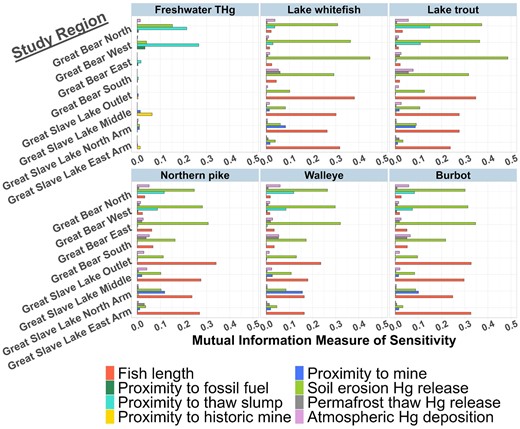
Barplots illustrating results of sensitivity analysis used to identify the Hg sources that are most influential on Hg concentrations in freshwater and fish. The mutual information measure of sensitivity is plotted on the x axis, and the eight different model study regions on the y axis. The plots are separated by the six Hg effect variables: the THg concentrations in freshwater and the tissue Hg concentrations in the five fish species. The colored bars represent the eight Hg sources across the Great Bear Subbasin (GBS) and Great Slave Lake (GSL) models. Variables with negligible mutual information values are not adequately described by any of the Hg pathways considered in the model frameworks.
The sensitivity analysis results further support the earlier discussion regarding which Hg sources are causing the elevated risk in the GBS South and GSL North Arm study regions. As predicted from the source node probability distributions, the high fish Hg concentrations in the GBS South were attributed to the three nonpoint Hg sources (Figure 4), and particularly, the greater influence of the atmospheric deposition and permafrost thaw Hg sources relative to the other GBS study regions. Similarly, the sensitivity analysis indicates that the GSL North Arm is unique in that it is the only region in the GSL model where mining proximity is highly influential to fish Hg concentrations (Figure 4). This corroborates the prediction that the high fish Hg concentrations are related to the greater active mining effort in the GSL North Arm compared with other areas of GSL, which is further supported by the slope coefficients and t-values of the regression models developed using fish Hg monitoring datasets (Table 2).
Objective 3: Counterfactual analysis
Counterfactual 1: Impact of Minamata Treaty
The Minamata Convention is a multilateral agreement to reduce the anthropogenic inputs of Hg into the environment; it was signed in 2013 by 128 countries that pledged to reduce Hg use across manufacturing, energy, and gold mining industries by 2030 (UNEP, 2019, 2021). Atmospheric Hg deposition is the dominant Hg source to the Arctic (Dastoor et al., 2022) and industrial activity in southern regions has resulted in the build-up of legacy Hg in permafrost, lake sediments, and Arctic soils. In Canada, where over 95% of the deposited anthropogenic Hg originates from other countries (Fraser et al., 2018), global management initiatives such as the Minamata Treaty are necessary to reduce Hg inputs.
A study by the Global Mercury Observation System project assessed three future Hg emission scenarios: a current (as of 2010) policy scenario, a new policies scenario, and the ambitious 450 [ppm] scenario. The 450 [ppm] climate-policy scenario corresponds to an ambitious goal for stabilized CO2 concentration of 450 parts per million and limiting global temperature increase to 2°C. In this idealistic 450 [ppm] scenario where all countries achieve the highest feasible reductions in Hg emissions, Hg deposition has been predicted to decrease by 35%–60% across the Mackenzie basin (Pacyna et al., 2016).
The GBS South region was selected for the counterfactual analysis aimed at examining the impact of the Minamata Treaty because of the high fish Hg concentrations there and the influence of atmospheric Hg deposition on fish Hg levels, as shown by sensitivity analysis (Figure 4). Over the past 20 years, the GEM-MACH-Hg model suggests that the GBS South region had moderate atmospheric Hg deposition rates, with approximately 90% of the atmospheric deposition values above 9 μg Hg m−2 yr−1, and 10% falling between 3 and 9 μg Hg m−2 yr−1 (Dastoor et al., 2015; online supplementary material Figure S8). Assuming the successful implementation of the Minamata Treaty and the 450 [ppm] climate scenario reductions in atmospheric Hg deposition rates, the future mean Hg deposition rates in the GBS South will be ∼4.8–7.7 μg Hg m−2 yr−1. A hypothetical scenario of an atmospheric deposition value between 3 and 9 μg Hg m−2 yr−1 was input into the model, affecting the distribution of downstream nodes (online supplementary material Figure S45a), including the fish Hg effect variables. Prior to the intervention, the average Hg concentrations in lake whitefish are 0.332 ± 0.32 μg/g and in northern pike was 0.938 ± 0.61 μg/g (online supplementary material Figure S8) but shift downwards to 0.231 ± 0.28 μg/g and 0.72 ± 0.54 μg/g, respectively, in the 450 [ppm] scenario (online supplementary material Figure S15). When the scenario is applied across all study regions and fish species, the average reduction in fish Hg concentrations was 1.2-fold under the 450 [ppm] climate scenario.
Contrary to the objective of the Minamata Treaty, global atmospheric Hg emissions increased by ∼20% between 2010 and 2015, driven by industrial growth in South America and Asia (Dastoor et al., 2022). To explore a scenario where atmospheric Hg emissions continue rising exponentially, a higher annual atmospheric Hg deposition rate of ≥ 15 μg/m2 was input into the model. In this scenario, the fish Hg concentrations increased to a mean of 0.489 ± 0.33 μg/g for lake whitefish and 1.20 ± 0.72 μg/g for northern pike (online supplementary material Figure S15). Across the eight study regions and five fish species, the increased atmospheric Hg deposition resulted in a 1.6-fold increase in fish Hg concentrations. The prediction that fish Hg concentrations will decrease with decreased Hg input from the atmospheric deposition pathway is compatible with our causal understanding of the Hg cycle (AMAP, 2011; AMAP/UNEP, 2015). If the BN modeling approach presented here, which connects abiotic Hg fate and transport to biotic Hg concentrations, is extended to other geographical regions with environmental Hg data (Evers et al., 2024) the resulting models could be valuable tools for future Minamata effectiveness evaluations.
Counterfactual 2: Impact of consuming smaller fish
In the NWT, site-specific fish consumption advice often includes a size restriction, with piscivorous fish over 600 mm being considered higher-risk food sources (GNWT Health and Social Services, 2016). This counterfactual query compared the probability that an adult male will exceed their Hg dietary threshold given that they consume one weekly portion (150 g fish) of either small (< 600 mm) or large (≥ 600 mm) northern pike. Because the fish Hg levels vary spatially, this counterfactual was performed for both the GSL Outlet (lower fish Hg concentrations) and the GSL North Arm (higher fish Hg concentrations). In both locations, the average fish Hg concentration was ∼two- to threefold higher for a large-sized northern pike (0.74 ± 0.39 μg/g in the Outlet; 0.93 ± 0.54 μg/g in the North Arm) than a small-sized pike (0.30 ± 0.28 μg/g in the GSL Outlet; 0.50 ± 0.37 μg/g in the GSL North Arm). The resulting probability of exceeding the Hg ingestion guidelines for adult males consuming a large fish (6.0% [Outlet] and 14.4% [North Arm] probability of exceedance) was three- to fivefold greater than for adult males who consume small fish (1.8% [Outlet] and 3.7% [North Arm] probability of exceedance; online supplementary material Figures S16 and S17). A diet of small-sized fish resulted in a 1.5- to fivefold reduction in risk for all five fish species and across all eight study regions. The model confirms that individuals who follow site-specific consumption advice issued by the NWT government are less likely to exceed the Hg dietary thresholds compared with individuals who continue to consume larger fish.
Evaluation of uncertainty and the Hg dataset completeness
Monitoring fish for Hg (Figure 1) was more prominent in the GSL study area than in the GBS (768 vs. 276 datapoints), resulting in greater uncertainty in the GBS model output for the fish Hg nodes. In contrast, fewer freshwater THg samples were collected in the GSL study regions (855 datapoints vs. the 1,271 in the GBS). In the GBS model, the locations of fish sampling sites were sparse and therefore not representative of the study region. For example, fish sampling in the GBS West and East study regions was limited to only a few southern-most waterbodies (Figure 1), resulting in a knowledge gap of the Hg concentrations in much of the study regions. Additionally, fish monitoring was practically nonexistent in the vicinity of RPTSs (8.8%) and fossil fuel developments (< 1%) located in the GBS North and West regions (online supplementary material Figure S1). The impact of the presence of these two point-sources on fish Hg concentrations was highly uncertain due to this gap in monitoring data.
The calculation of the degree of Hg-induced fish injury is another source of uncertainty in the model predictions, because the dose-response curves were developed based on toxicological experiments on juvenile fathead minnows. As fathead minnows are believed to be less sensitive to metal toxicity than other fish species (particularly salmonid species like lake trout and lake whitefish), the model dose-response curves are likely resulting in an underestimation of the degree of injury to the five fish species in the BN-RRMs (Dillon et al., 2010).
The use of environmental models to inform the Hg nonpoint source nodes is a source of epistemic uncertainty in the BN-RRM output. The predictions from the atmospheric Hg deposition (Dastoor et al., 2015) and permafrost thaw Hg release (Schaefer et al., 2020) environmental models are themselves highly uncertain, as illustrated by their low resolution (raster resolution of ∼1874 km2, online supplementary material Table S3 and Figure S2). Much of this uncertainty is caused by gaps in monitoring data and a lack of knowledge of the processes that govern Hg transport and transformation between its numerous forms. Additionally, the soil erosion (RUSLE) calculation used equations that were developed for temperate climates and European vegetation, which are very different from the boreal forests and tundra ecosystems of the Mackenzie River watershed. Furthermore, there are currently no studies that have quantified how permafrost depth and continuity affect the RUSLE calculation. The development of an Arctic-specific RUSLE calculation would reduce the uncertainty and assumptions associated with the estimation of soil erosion as a Hg source.
Future research recommendations
Several future research recommendations were developed from data gaps identified during the development of the BN-RRM (Figure 5), including compiling and mapping sampling locations and available datatypes (categorized as monitoring research gaps; see online supplementary material Figure S14, which illustrates data completeness), and through reviewing literature that describes gaps in Hg transfer dynamics (categorized as process-driven research).
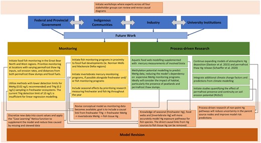
Future research recommendations developed from data gaps identified by a Bayesian network model of Hg exposure in the Mackenzie watershed. The chart is organized into long-term monitoring and shorter-term process-based research. The additional data resulting from implementation of these recommendations will allow for revisions to the model and reduce the uncertainty from sampling bias and lack of knowledge of causal pathways.
Monitoring recommendations include the adoption of freshwater THg analysis methods with a lower detection limit (0.2 ng/L), the inclusion of invertebrate monitoring in freshwater and fish monitoring programs (Moslemi-Aqdam et al., 2022), and the development of a fish monitoring program in Norman Wells to better understand how fossil fuel exploration is affecting fish health and Hg levels (Imperial Oil Resources Ltd, 2022). Process-driven research recommendations focused on expansions of modeling efforts to improve understanding of methylation potential, quantify the extent to which permafrost presence and continuity stabilizes against soil erosion, and integrate climate projections or future socioeconomic scenarios into future BN models (Figure 5).
We also recommend that alternate BN models are developed in collaboration with rights-holders and stakeholders, as this is one method of reducing epistemic uncertainty and validating BN-RRMs (Sahlin et al., 2021). Developing multiple conceptual diagrams ensures that the model structure and discretization agrees with available knowledge and that the model endpoints illustrate the needs of the end users, creating increased trust in the model output (Kaikkonen et al., 2021). The development of hybrid BN models, which combine continuous and discrete variables (Kaikkonen et al., 2021), may also reduce epistemic uncertainty arising from discretization (Nojavan et al., 2017). Although justification for discretization based on MRB-specific scientific knowledge was applied when available, some variables (i.e., nonpoint sources) may be better represented as continuous nodes, given a lack of studies to inform class boundary selection (online supplementary material Table 4).
Finally, there is epistemic uncertainty associated with the discretization of the study area into eight study regions, which describe relatively large and heterogeneous landforms (∼21,000 km2–160,000 km2, Table 1) spanning several subcatchments. There are tools that enable the development of spatially and temporally explicit BN models (Stritih et al., 2020) where the model is run on a smaller and more homogeneous scale, such as individual pixels of a raster. Linking the static BN models with spatial software would yield results on scales that are more relevant for ecosystem management projects, whereas the visual component aids stakeholders and policymakers in accessing and interpreting the output (Glendell et al., 2022; Stritih et al., 2020).
Conclusion
The BN-RRMs developed during this research showcase the strength of BN models as powerful probabilistic models capable of consolidating different types of data and information from a variety of scientific disciplines and ecosystem management projects. For the first time, the outputs of several contemporary Hg modeling studies were integrated into a single model framework, including environmental models for atmospheric Hg deposition, permafrost thaw, and soil organic content. Furthermore, high-resolution satellite imagery of vegetation density and elevation were used in a novel calculation of Hg released due to rainfall-induced soil erosion (online supplementary material Figures S3, S12, and S18). The Hg sources, described by proximity nodes and the environmental models’ outputs, were connected to observed Hg concentrations in freshwater and biota obtained from 21 monitoring projects. Finally, environmental Hg concentrations were used to quantify risk to endpoints that are relevant for community members (i.e., probability of exceeding dietary Hg intake guidelines) and small commercial fishing operations present throughout the MRB (i.e., probability of Hg-induced fish injury and probability of fish catch exceeding Hg commercial sale thresholds).
The BN-RRMs were also used to compare the impact of two risk-mitigation strategies: the Minamata Treaty to reduce atmospheric Hg release and advice to limit the intake of larger and more-predatory fish. The models predicted that successful implementation of the Minamata Treaty and an ambitious 450 [ppm] greenhouse gas emissions scenario, corresponding to 35%–60% reduction in atmospheric Hg deposition across the MRB, would translate to a ∼1.2-fold reduction in fish Hg concentrations. However, in the scenario where Hg and greenhouse gas emissions continue to increase such that the MRB begins to experience annual Hg deposition rates ≥ 15 μg Hg/m2, the fish Hg concentrations are expected to increase by ∼1.6-fold.
With the first Minamata Effectiveness Evaluation currently underway and several future evaluations expected, there is a need for models that can inform policymakers on the impact and progress of the Minamata Treaty. Models such as this one, which link atmospheric Hg deposition to Hg levels in the environment, are valuable tools for comparing current and future effectiveness evaluations while accounting for inputs from other Hg sources. These BN-RRMs are visual models that explicitly communicate the current knowledge of environmental Hg in the Mackenzie River and GSL. These models can empower individuals in the Canadian Northwest Territories by raising awareness about how Hg inputs from a variety of nonpoint and point sources can affect Hg levels in country foods.
Supplementary material
Supplementary material is available online at Integrated Environmental Assessment and Management.
Data availability
All data (including metadata and R script) are publicly available in the supplemental information and the Federation Research Data Repository (Doi: 10.20383/103.0957).
Author contributions
Una Jermilova (Data curation, Formal analysis, Investigation, Visualization, Writing—original draft), Jane Kirk (Conceptualization, Funding acquisition, Supervision, Writing—review & editing), S. Jannicke Moe (Methodology, Resources, Software, Supervision, Validation, Writing—review & editing), Wayne Landis (Methodology, Resources, Supervision, Validation, Writing—review & editing), Emma Sharpe (Methodology, Writing—review & editing), Maeve McGovern (Formal analysis), Hans Fredrik Braaten (Funding acquisition, Project administration, Resources), Cathrine Gundersen (Funding acquisition, Project administration, Resources), Ashu Dastoor (Data curation, Resources, Writing—review & editing), Kevin Schaefer (Data curation, Resources), Holger Hintelmann (Project administration, Supervision, Writing—review & editing)
Funding
Initial funding for the ARCRISK project (project number 190204) was funded by the Arctic Contaminants Action Program (ACAP) and the Arctic Council Project Support Instrument (PSI) and is co-sponsored by the Norwegian Ministry of Climate and Environment (KLD). The Nordic Environment Finance Corporation (NEFCO) is the fund manager. Subsequent funding was provided by Global Affairs Canada (project number P-013920).
Conflicts of interest
The authors declare no conflict of interest.
Disclaimer
The peer review for this article was managed by the Editorial Board without the involvement of S. Jannicke Moe.
Acknowledgments
Environmental models were graciously shared by Camile Sothe (McMaster University and World Wildlife Fund Canada), Kevin Schaeffer (National Snow and Ice Data Center, University of Colorado Boulder), and Ashu Dastoor (Environment Climate Change Canada) through private correspondence. Publicly available mercury monitoring data were obtained from the Mackenzie DataStream (https://mackenziedatastream.ca/), and the following individuals: Mary Gamberg (Northern Contaminants Program funded projects), David Depew (Canadian Fish Mercury Database), and Aimee Guile (Wek’èezhìı Renewable Resources Board).
