


Abstract
Common sole (Solea solea) is a key commercial flatfish species in Europe, yet its stock identity in the southern Celtic Sea and southwest of Ireland (ICES area 7h and 7j) is uncertain, resulting in a precautionary approach to fisheries management and declining quota. Here, the structure of sole populations and their connectivity patterns were investigated from the southern North Sea to the Bay of Biscay spanning 10 ICES areas using 55 706 single nucleotide polymorphisms and five biological variables (sex, maturity, age, length, and weight). Our results confirmed the large-scale genetic differentiation between sole in the southern North Sea (ICES area 4c) and Bay of Biscay (8a, 8b). Sole from area 7h was genetically similar to sole from the Celtic Sea (7f and 7g) (both neutral and outlier loci), Western English Channel (7e, only neutral loci), and Irish Sea (7a, only neutral loci). Sole from area 7j showed significant neutral differentiation with sole from areas 7h and 7g, the Western English Channel (7e), and the Irish Sea (7a). These novel insights suggest a current mismatch between the biological populations and stock units of 7h and 7j, currently managed as a single stock, and provide a crucial basis for the re-evaluation of the current stock status, enabling more informed and effective fisheries management.
Introduction
Stock assessments require high-quality, reliable, and sufficient data to facilitate optimal estimations of the stock status (Carvalho and Hauser 1995, Begg et al. 1999). Overexploitation results in loss of productivity as documented across a wide range of marine fishes and might even destabilize local and regional stock dynamics (Pinsky and Palumbi 2014, Kerr et al. 2017). In addition, declining population sizes and reduced genetic diversity in exploited commercial species could hamper the potential of natural populations to adapt to changing environments (Markert et al. 2010, Pearse 2016, Gandra et al. 2021). Therefore, the correct identification of the population structure and connectivity among populations is imperative for the long-term conservation and sustainable management of commercial fisheries (Andersson et al. 2024). For many marine fishes, however, populations are delineated as stocks based on management criteria. Consequently, for several fisheries, these populations (biological units) are often and roughly mismatched by management units (stocks), which impacts assessments and predictive modelling (Reiss et al. 2009, Casey et al. 2016).
Several factors influence genetic isolation among marine fish populations, including geographic and oceanic distance, environmental gradients (e.g. temperature, salinity), bathymetric boundaries, life-history variants (e.g. ecotypes), and historical factors (e.g. the last ice age, overfishing) (Bossart and Prowell 1998, Salmenkova 2011). Marine fish populations are typically large, which limits the effects of genetic drift and reduces divergence at neutral markers (Hellberg et al. 2002, Cano et al. 2008). The use of single nucleotide polymorphisms (SNPs) revealed previously hidden levels of genetic diversity among marine flatfish populations, as demonstrated in plaice Pleuronectes platessa (Le Moan et al. 2021, Weist et al. 2022) and flounder Platichthys flesus (Kuciński et al. 2023).
One of the most important commercial demersal marine fish species in Europe is the common sole, Solea solea (Linnaeus 1758, Pleuronectiformes, hereafter referred to as sole) (Millner et al. 2005, Bjørndal et al. 2016, Jayasinghe et al. 2017). Sole has a broad geographical distribution in the Eastern Atlantic Ocean from the northwest coast of Africa to Senegal (15°N), in almost all of the Mediterranean Sea to southern Norway (60°N), Kattegat, and the Western Baltic Sea. This flatfish is often semi-immersed in the muddy or sandy seabed (Whitehead et al. 1984, Quéro et al. 1986) and spawns in shallow (<30 m depth) areas from early February to June, largely triggered by sea surface temperature (Russell 1976, Borremans 1987). The onset of spawning usually occurs at temperatures ranging from 8°C to 10°C (Devauchelle et al. 1987). The large number of pelagic eggs (estimates ranging from 200 000 to 440 000 per female) and settling of pelagic larvae ∼3 weeks after hatching in nursery areas may prevent strong population structuring (Witthames et al. 1995). In contrast, some studies argue that larval connectivity is weak as spawning areas are restricted to estuarine and coastal nursery grounds (Rochette et al. 2012). Furthermore, movement of juveniles at their nursery grounds is limited (<10 km) resulting in little connectivity from juvenile movement (Coggan and Dando 1988, Le Pape and Cognez 2016). Adult movement could be a potentially important driver of gene flow between populations (Frisk et al. 2014). Yet, homing behaviour might favour reproductive isolation and thus divergence between populations (Exadactylos et al. 2003).
Several studies have investigated the population structure of sole using a variety of genetic markers: allozymes (Kotoulas et al. 1995, Exadactylos et al. 1998), isozymes (Cabral et al. 2003), Random Amplified Polymorphic DNA (Exadactylos et al. 2003), mitochondrial DNA (Guarnieo et al. 2002, Rolland et al. 2007), microsatellites (Cuveliers et al. 2012), and more recently SNPs (Diopere et al. 2018, Corti et al. 2024). Based on neutral microsatellites and mitochondrial markers, genetic differences along a latitudinal gradient in the North-East Atlantic were documented with at least three distinct populations: Kattegat/Skagerrak, North Sea, and Bay of Biscay, with indications of a fourth population in the Irish/Celtic Sea (Cuveliers et al. 2012). Genome-wide SNP fingerprinting confirmed the previously found population structure and the existence of an Irish/Celtic Sea group and showed additional sub-structuring between the North Sea and English Channel (Diopere et al. 2018). In addition, tagging revealed limited adult movement between the Western English Channel, Eastern English Channel (split into three discrete sub-areas) and the North Sea (Lecomte et al. 2020). The population structure of sole in the southern Celtic Sea and southwest of Ireland (ICES area 7hjk), however, remains unknown despite its large economical potential for the sole fishing industry. The lack of information on the stock identity of sole in this region contributes to the implementation of the precautionary principle by the International Council for the Exploration of the Sea (ICES) (ICES 2012, ICES 2022). As a result, ICES catch advice is reduced by 20% every three years in the region, causing a detrimental socio-economic impact on the commercial fishing fleet.
In this study, we investigated the genetic population structure and connectivity patterns of adult sole in the North-East Atlantic over a gradient from 45.25°N to 53.75°N spanning 10 ICES areas from the southern North Sea to Bay of Biscay using 55 706 high-quality SNP markers. These results were complemented with biological data obtained from the genetically analysed fish (sex, maturity, age, length, weight) to investigate if underlying biological patterns could affect the detected population genetic structure. Specific focus was on unravelling the genetic structure of sole in the data poor areas in the southern Celtic Sea (7h) and southwest of Ireland (7j) to evaluate whether the precautionary principle in current stock management is warranted.
Materials and methods
Sample collection
A total of 541 sole were collected during the first and second quarters (January to June) of 2022 on board Belgian commercial fishing vessels in the framework of the Belgian National Data Gathering Program (NDGP) using beam trawls (80 mm mesh size). The target number of sole per ICES statistical rectangle was 20 individuals. Four rectangles were sampled in 7d, three rectangles in 4c, 7h, 7f, 7g, and 7a, and the combined areas of 8a and 8b, two rectangles in 7e and one rectangle in 7j (Fig. 1, Table 1). Although sole are currently managed under stock 7hjk, no samples were included from ICES area 7k due to the region’s bathymetry, which makes it a largely unsuitable habitat for sole. Consequently, fisheries targeting sole are absent in this area. Fish were morphologically identified by experts on board. Every fish was stored in a separate plastic bag to avoid contamination of DNA between fish, labelled, and transported to the laboratory on ice. Length, weight, sex, and maturity of each fish were recorded, and otoliths were extracted for age determination using the sectioned and stained method (Table 1) (Easey and Millner 2008). The age of 16 collected sole could not be determined, resulting in a total of 525 sole with five complete biological parameters (i.e. length, weight, sex, maturity, and age). Of those 525 individuals, a subset of 361 samples was used for genetic analyses.
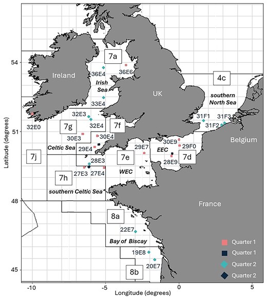
Map with sampling locations of sole in quarter one (square shape) and quarter two (diamond shape) of 2022 with ICES areas (black lines) and statistical rectangles (grey lines). The colours of the sampling points represent the type of data used in this study: biological and genetic data (pink and light blue) and only biological data (dark blue).
Sampling information includes location, abbreviation (Code), ICES area and rectangle (Rec), coordinates in latitude (Lat), and longitude (Lon) and date (day/month in 2022), number of individuals genotyped (N), mean weight of genotyped fish (g) with minimum and maximum (min–max), mean length (cm) with min–max, and mean age (year) with min and max.
| Location | Code | ICES area | Rec | Lat | Lon | Date | N | Mean weight (min–max) | Mean length (min–max) | Mean age (min–max) | HO | HE | FIS |
|---|---|---|---|---|---|---|---|---|---|---|---|---|---|
| Southern North Sea | 4c | 31F1 | 51.48 | 1.68 | 02/05 | 14 | 114.1 (17.6–289.8) | 239.1 (140–326) | 4.2 (1–8) | 0.26 | 0.27 | 0.04 | |
| NOS | 31F2 | 51.27 | 2.96 | 29/06 | 18 | 103.5 (60.0–167.7) | 227.9 (190–264) | 2.4 (1–5) | 0.26 | 0.27 | 0.04 | ||
| 31F3 | 51.34 | 3.13 | 29/06 | 15 | 110.9 (43.3–207.8) | 230 (177–285) | 2.3 (1–4) | 0.26 | 0.27 | 0.03 | |||
| Eastern English Channel | 7d | 28E9 | 49.95 | −0.50 | 05/01 | 15 | 196.9 (96–340) | 276.7 (226–347) | 5.1 (2–14) | 0.26 | 0.27 | 0.03 | |
| EEC | 29F0 | 50.40 | 0.15 | 02/02 | 6 | 166.7 (117.8–227.0) | 277.7 (256–305) | 5.4 (4–6) | 0.26 | 0.27 | 0.03 | ||
| 30E9 | 50.65 | 0.00 | 14/03 | 16 | 81.1 (42.6–144.4) | 219.7 (186–255) | 2.9 (2–5) | 0.26 | 0.27 | 0.04 | |||
| Western English Channel | WEC | 7e | 28E3 | 49.58 | −6.12 | 23/04 | 8 | 237.3 (111.5–436.2) | 303.6 (255–375) | 5 (3–9) | 0.26 | 0.27 | 0.03 |
| 29E7 | 50.07 | −2.37 | 08/03 | 15 | 535.4 (307–943.5) | 386.1 (323–459) | 7.8 (4–11) | 0.25 | 0.27 | 0.04 | |||
| Irish Sea | 7a | 33E4 | 52.47 | −5.07 | 30/04 | 17 | 249.7 (74.6–704.6) | 289.3 (205–426) | 4.6 (2–16) | 0.26 | 0.27 | 0.04 | |
| IRE | 36E4 | 53.77 | −5.13 | 01/05 | 12 | 132.5 (52.4–478.5) | 246.9 (201–359) | 4.3 (2–6) | 0.26 | 0.27 | 0.04 | ||
| 36E6 | 53.89 | −3.62 | 30/03 | 14 | 156.5 (49.9–508.4) | 249.4 (188–357) | 4.1 (2–8) | 0.26 | 0.27 | 0.04 | |||
| Celtic Seas | 7g | 30E3 | 50.90 | −6.55 | 23/01 | 11 | 243.7 (153.7–391.2) | 293 (264–332) | 5.7 (4–7) | 0.26 | 0.27 | 0.03 | |
| 32E3 | 51.65 | −6.15 | 26/05 | 17 | 166.8 (67.2–505.6) | 265.8 (201–375) | 3.3 (2–6) | 0.26 | 0.27 | 0.04 | |||
| 32E4 | 51.57 | −5.93 | 28/05 | 12 | 165.5 (79.6–526.5) | 257.0 (217–396) | 3 (2–8) | 0.26 | 0.27 | 0.04 | |||
| CEL | 7f | 29E4 | 50.33 | −5.73 | 11/03 | 20 | 352.3 (141.5–1423) | 330 (259–501) | 6.4 (4–18) | 0.26 | 0.27 | 0.04 | |
| 30E4 | 50.80 | −5.55 | 21/01 | 6 | 172.4 (121.7–241.5) | 273.7 (256–295) | 5.6 (4–8) | 0.26 | 0.27 | 0.02 | |||
| 7h | 27E3 | 49.45 | −6.52 | 09/02 | 17 | 298.4 (140.8–598.1) | 317.1 (263–393) | 5.5 (3–9) | 0.25 | 0.27 | 0.04 | ||
| 27E4 | 49.43 | −5.07 | 08/02 | 7 | 357.7 (223.4–518.8) | 343.1 (307–376) | 6 (5–9) | 0.26 | 0.27 | 0.03 | |||
| Southwest Ireland | SWI | 7j | 32E0 | 51.80 | −9.84 | 25/01 | 33 | 341.3 (70–722) | 302 (200–400) | 5.8 (2–11) | 0.26 | 0.27 | 0.03 |
| Bay of Biscay | 8a | 22E7 | 46.65 | −2.97 | 30/05 | 19 | 159.5 (76.9–388.9) | 267.5 (223–365) | 4.5 (2–15) | 0.26 | 0.27 | 0.04 | |
| BISC | 8b | 19E8 | 45.27 | −1.63 | 28/06 | 16 | 188.2 (59.9–353.3) | 277.2 (214–350) | 4.9 (2–13) | 0.26 | 0.27 | 0.04 | |
| 20E7 | 45.68 | −2.03 | 2/06 | 16 | 183.2 (66.9–456.9) | 281.5 (221–381) | 5.8 (3–11) | 0.26 | 0.27 | 0.04 |
Following genetic diversity measures are provided per ICES rectangle: observed and expected heterozygosity (HO and HE, respectively) and inbreeding coefficient FIS. Genetic diversity measures per ICES area can be consulted in Table S1.
DNA extraction and GBS library preparation
Individual genomic DNA was extracted from muscle tissue (after removal of skin) with the spin-column protocol for purification of total DNA from animal tissues using the DNeasy Blood & Tissue Kit (Qiagen, Germany). DNA concentrations were estimated using the Quantus Fluorometer dsDNA System (Promega, USA). First, DNA samples were diluted to 10 ng/µl (although samples with a concentration >7 ng/µl were retained for further analyses as well). The GBS libraries were prepared following a modified version of the genotyping-by-sequencing protocol by Poland and Rife (2012) using restriction enzymes PstI and MspI. The master mix for one sample for the restriction digestion consisted of 2 µl rCutSmart Buffer (NEB), 7 µl Sigma H2O, 10 units of PstI (NEB), 10 units of MspI (NEB), and 10 µl template DNA. Samples were incubated for 2 h at 37°C. No heat inactivation step was performed during incubation in contrast with the original protocol. For the ligation step, the master mix for one sample was composed of 200 units of T4 DNA ligase (NEB), 2 µl T4 DNA ligase buffer (NEB), 7 µl H2O, and 1.5 µl of Y-shaped common adapter (10 µM). Per sample, 20 µl restriction digest and 4 µl barcoded adapters (0.25 µM) were added. Samples were incubated at 22°C for 2 h, followed by 65°C for 20 min. The first purification step was repeated to remove all primer dimers with CleanNGS (CleanNA) using a volume ratio of 1.6 beads: 1 DNA. Next, each PCR reaction consisted of 12.5 µl Taq 2x Master Mix (NEB), 5.5 µl H2O, 3 µl purified digested DNA, 2 µl unique P5 primer (10 µM), and 2 µl unique I7 primer (10 µM). The following PCR conditions were used: 30 s at 95°C, followed by 18 cycles of 30 s at 95°C, 20 s at 65°C, and 30 s at 68°C. For the purification of the PCR amplicons, 10 µl H2O was added to each amplicon, followed by a purification identical to the first purification step. Next, samples were quantified using the Quantus Fluorometer dsDNA System, and the quality of a random subset of samples was checked with the Bioanalyzer 2100. To account for potential sequencing bias, replicate samples were included on all separate sequencing runs. After final quantification and quality checking, samples were pooled with equal volume (5 µl) for the first run on the HiSeqX 2 × 150 bp platform (128 samples, including 8 replicates in pool 1) and Novaseq 6000 (283 samples, including 20 replicates in pool 2 and 64 samples, including 20 replicates in pool 3). For the second run, all samples with <3 million reads and more than 30 000 clusters were re-sequenced on the HiSeq X 2 × 150 bp platform (pools 1, 2, and 3) after pooling with modified volume. More details on the calculation of the modified volume can be consulted in Appendix 1.
Bioinformatics, SNP calling, and filtering
Initial processing of reads (i.e., demultiplexing, trimming and merging of forward and reverse reads) was done using GBprocesS v4.0.0 (see https://gbprocess.readthedocs.io/). Reads were mapped against the Solea solea reference genome (GenBank: GCA_958295425.1) using BWA (Li et al. 2009). Variant calling was done using the mpileup command in BCFtools (Danecek et al. 2021). SNPs were filtered using VCFtools (Danecek et al. 2011) with the following parameters: (1) Minor Allele Frequency (MAF) 0.05; (2) only SNPs with two alleles and (3) minimum depth 15. Individuals and loci with more than 10% missing data were filtered from the dataset using the R package poppr v2.9.3 (Kamvar et al. 2014). Loci with observed heterozygosity >0.50 were excluded from the dataset as they might be derived from collapsed paralogous loci in the reference sequence (Hohenlohe et al. 2011). Loci deviating from Hardy-Weinberg proportions (p < 0.05) calculated for each population separately (i.e., ICES level) were removed. Replicate samples included on separate sequencing runs were used to detect potential library or sequencing bias based on PCA clustering and removed from the dataset to avoid redundancy.
Outlier detection
Outlier SNPs (SNPs potentially under selection) were identified using two outlier detection methods: R package pcadapt v4.3.3 for outlier detection based on Principal Component Analysis (PCA) (Luu et al. 2017) and OutFLANK for outlier detection based on FST that were more divergent than expected under neutrality using R package dartR v2.0.4 (Gruber et al. 2018). For pcadapt, the optimal K (ranging from 1 to 20) was assessed, followed by two outlier detection methods with several cutoffs: (1) outliers detected with threshold 0.05 and 0.1 after Bonferroni correction; (2) outliers detected after calculation of false discovery rate (FDR) of the obtained P-values with threshold 0.05 and 0.1 using the q-value function with R package q-value v2.30.0. OutFLANK was run with default options (LeftTrimFraction and RightTrimFraction = 0.05, Hmin = 0.1) and q-value thresholds for statistical significance set at 0.05 and 0.1. For each outlier detection method, a Manhattan plot visualizing outlier SNPs exceeding the FDR with threshold q = 0.05 was obtained. Outlier detection methods were compared to obtain the shared outlier SNPs.
Genetic data analysis
Population diversity measures and patterns were investigated on two levels: (1) 10 ICES areas 7d, 7f, 7g, 7h, 7e, 7a, 4c, 8a, 8b, and 7j, and (2) statistical rectangles within and between each ICES area. Mean observed (HO) and expected (HE) heterozygosity and inbreeding coefficient (FIS) per ICES area were calculated using R package hierfstat v0.5.11 (Goudet 2005). Pairwise FST values with 99% confidence intervals and P-values were estimated with R package StAMPP v1.6.3 using 10 000 bootstraps (Pembleton et al. 2013) for both the neutral and outlier SNPs dataset. P-values were adjusted for multiple testing by applying Bonferroni correction. To investigate patterns of population structure, three methods were used for grouping sole individuals using the neutral and outlier SNPs dataset: PCA, discriminant analysis of principal components (DAPC), and admixture analysis. DAPCs were created using R package adegenet with a priori defined groups (i.e. management units; ICES areas and rectangles).To avoid inaccurate interpretations of the observed population structure caused by sex-linked markers, structuring based on sex (male, female), maturity (immature, maturing, spawning, and spent) and age (ranging from 1 to 18 years), was investigated for both the neutral and outlier datasets using PCA. Admixture proportions per clusters based on statistical rectangles were calculated in R package LEA v3.10.0 (Frichot and François 2015) with the sparse non-negative matrix factorization algorithm at individual and population level for the neutral and outlier SNPs dataset. Admixture proportions were visualized as pie charts using R package Mapmixture v1.0.4 (Jenkins 2024).
Isolation-by-distance
A Mantel test was performed to investigate the presence of isolation-by-distance (IBD) by testing for correlations between genetic distance (neutral pairwise FST) and oceanic distance (km) between populations. Pairwise oceanic distances (marine least-cost distances via coast) between sampling locations were calculated using function lc.dist in R package marmap v1.0.10 (Pante and Simon-Bouhet 2013). The Mantel test was conducted using the mantel function in R package vegan v2.6.4 (Oksanen et al. 2022).
Identification of candidate genes
The physical position of the shared outlier SNPs (identified by both outlier detection methods pcadapt, and OutFLANK) was used to identify the potential candidate genes under selection on the annotated Solea solea reference genome (assembly fSolSol10.0 with 37 228 genes) using the Genome Data Viewer on NCBI (Rangwala et al. 2021). For each gene with at least one outlier SNP in its coding region, the gene name, gene ID, brief description of its function, and location on the genome were documented. Outlier SNPs shared between the two outlier methods were visualized on a Manhattan plot using the function manhattan in R package qqman v0.1.8 (Turner 2018).
Variation in biological variables
The biological metadata obtained from 525 sole specimens were analysed, and length, weight, and age for sole collected in each of the 10 ICES areas were visualized. Linear mixed-effects regression models were employed to examine length and weight, incorporating both fixed (ICES areas) and random effects (sex and age) using the R package lme4 v1.1-35.3 (Bates et al. 2016). The fixed effect allowed to estimate how average length and weight vary across these areas. The random effects accounted for variability in length and weight related to sex and age.
The bootMer function from the R package boot v1.3-30 (Canty 2002) was used to obtain robust estimates of uncertainty for the model parameters, an approach that relaxes assumptions of normality and independence that parametric methods rely on (Davison and Hinkley 1997, Morris 2002). Post-hoc pairwise comparisons (Tukey’s test) were conducted using the R multcomp package v1.4-25 (Hothorn et al. 2008) to evaluate differences in length and weight across ICES areas.
Results
Bioinformatics and filtering
Filtering with VCFtools kept 60 484 SNPs with sufficient read depth. 41 replicate samples were removed after confirming that no library or sequencing bias occurred (Fig. S1). 983 SNP loci and 37 individuals contained missing values >10% and were removed from the dataset. 63 and 2328 SNP loci with, respectively, expected and observed heterozygosity above 50%, as well as 1404 SNP loci out of Hardy–Weinberg equilibrium, were removed from the dataset. The final dataset contained 55 706 SNP genotype calls in 324 individuals.
Outlier detection
An overview of the number of obtained candidate outlier SNPs detected by the two different outlier detection methods with different threshold is provided in Table S2. For pcadapt, K = 2 was retained after assessment using a scree plot of the proportion of variance explained by each PC. A total of 76 outlier SNPs obtained in both methods following FDR-adjusted q-values with threshold 0.05 were used for subsequent analyses. The Manhattan plots with outlier SNPs obtained through the chosen threshold in pcadapt and Outflank are provided in Fig. S2. The final neutral and outlier SNPs dataset contained 324 individuals with 55 630 and 76 SNP loci, respectively.
Genetic diversity and population differentiation
Observed and expected heterozygosity, with mean values of 0.25 and 0.27, respectively (t = 107.0, P < .001), were similar across all sampling sites. The inbreeding coefficient FIS was low with values ranging from 0.02 to 0.04 (Table 1). There was no evidence of population structuring based on sex, maturity, or age based on the neutral (Fig. S3) and outlier SNP dataset (Fig. S4).
Large scale population patterns: ICES areas
Neutral SNPs dataset
Pairwise FST values between ICES regions were low and varied from 0 to 0.0024 (Table 2). Sole sampled in the Bay of Biscay (8a and 8b) and southern North Sea (4c) were significantly differentiated from all other locations. No significant genetic differentiation was found for sole sampled in the Celtic Sea (7f, 7g, and 7h), nor was there significant differentiation between sole in the Western English Channel (7e), and the Eastern English Channel (7d), and sole from the Western English Channel (7e), Celtic Sea (7f, 7g, and 7h), and Irish Sea (7a). Sole from the southwest of Ireland (7j) was significantly differentiated with all other ICES areas, except for 7f in the Celtic Sea. When applying a less stringent threshold (P < .05), however, sole from area 7f was also significantly differentiated with area 7j (P = .02). The highest level of significant genetic differentiation was found between the southern North Sea (4c) and Bay of Biscay (8b, FST = 0.0024). Similarly, the PCA and DAPC showed the largest differentiation between sole from the Bay of Biscay and the southern North Sea along the first discriminant axis (Fig. 2a and b).
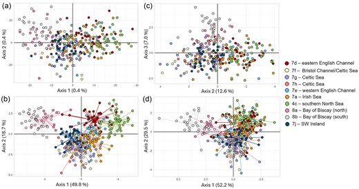
Population genetic structure based on (a and c) PCA and (b and d) DAPC of putative sole groups based on ICES areas after retaining the first (a and c) 50 PCs, (b) 100 PCs, and (d) 20 PCs, respectively, using the (a and b) neutral SNPs and (c and d) outlier SNPs dataset. Each dot represents an individual. The colours refer to ICES areas in which sole were collected. The PCA for the outlier dataset with PC axes 1 and 2 can be found in Fig. S4A.
Pairwise fixation index (FST) values (lower diagonal) for putative sole groups based on ICES areas and neutral SNP markers after 10 000 bootstraps and Bonferroni correction.
| EEC | CEL | CEL | CEL | WEC | IRE | NOS | BISC | BISC | |
|---|---|---|---|---|---|---|---|---|---|
| 7d | 7f | 7g | 7h | 7e | 7a | 4c | 8a | 8b | |
| 7f | 0.0008* | ||||||||
| 7g | 0.0006* | 0 | |||||||
| 7h | 0.0009* | 0 | 0.0001 | ||||||
| 7e | 0 | 0.0004 | 0.0002 | 0.0004 | |||||
| 7a | 0.0004* | 0.0002 | 0.0003* | 0.0005* | 0.0002 | ||||
| 4c | 0.0004* | 0.0011* | 0.0011* | 0.0013* | 0.0006* | 0.0007* | |||
| 8a | 0.0013* | 0.0013* | 0.0011* | 0.0011* | 0.0012* | 0.0014* | 0.0022* | ||
| 8b | 0.0015* | 0.0010* | 0.0013* | 0.0011* | 0.0014* | 0.0016* | 0.0024* | 0.0004 | |
| 7j | 0.0008* | 0.0005 | 0.0004* | 0.0006* | 0.0006* | 0.0007* | 0.0014* | 0.0012* | 0.0012* |
P-values < .01 are indicated with an asterisk (*).
Outlier SNPs dataset
Pairwise FST values estimated with outlier SNPs ranged from 0 to 0.0856, with the highest level of adaptive genetic differentiation between sole in the Bay of Biscay (8b) and southern North Sea (4c) (Table 3). Sole from the Bay of Biscay (8a and 8b) showed significant differentiation from all other ICES areas. Similar to the neutral FST values, no adaptive differentiation was observed between sole from the Celtic Sea (7f, 7g, and 7h), the Western English Channel (7e), and Eastern English Channel (7d), and between the Celtic Sea (7f, 7g, and 7h) and the Irish Sea (7a). Moreover, no adaptive genetic differentiation was detected in the greater Celtic Seas region (7f, 7g, 7h, 7a, 7e) and the southwest of Ireland (7j). The PCA with axes 1 and 2 based on outlier SNPs revealed no clear geographic structuring (Fig. S4); however, the PCA with axes 2 and 3 revealed a more similar pattern to the PCA based on neutral SNPs with the subtle grouping of the Bay of Biscay samples (8a, 8b) and Celtic Sea and southwest of Ireland samples (7h, 7f, 7g, and 7j). The Eastern English Channel (7d), Western English Channel (7e), Irish Sea (7a), and to some extent southern North Sea (4c) sole were separated along the x-axis (Fig. 2c). The DAPC based on outlier SNPs showed a clear separation of most sole sampled in the Bay of Biscay, particularly the southern part (8b), and all other locations (Fig. 2d). Furthermore, the DAPC based on outlier SNPs revealed similar patterns as the DAPC based on neutral SNPs, although the clustering of sole from the southern North Sea (4a), Eastern English Channel (7d), Western English Channel (7e), and Irish Sea (7a) was more pronounced in the DAPC with outlier SNPs.
Pairwise fixation index (FST) values (lower diagonal) for putative sole groups based on ICES areas and outlier SNP markers after 10 000 bootstraps and Bonferroni correction.
| EEC | CEL | CEL | CEL | WEC | IRE | NOS | BISC | BISC | |
|---|---|---|---|---|---|---|---|---|---|
| 7d | 7f | 7g | 7h | 7e | 7a | 4c | 8a | 8b | |
| 7f | 0.0635* | ||||||||
| 7g | 0.0417* | 0.0020 | |||||||
| 7h | 0.0352* | 0.0026 | 0 | ||||||
| 7e | 0.0027 | 0.0293 | 0.0140 | 0.0102 | |||||
| 7a | 0.0034 | 0.0271 | 0.0134 | 0.0087 | 0 | ||||
| 4c | 0.0029 | 0.0679* | 0.0579* | 0.0481* | 0.0133 | 0.0132* | |||
| 8a | 0.0534* | 0.0454* | 0.0481* | 0.0424* | 0.0308* | 0.0376* | 0.0506* | ||
| 8b | 0.0851* | 0.0722* | 0.0774* | 0.0771* | 0.0582* | 0.0715* | 0.0856* | 0.0101 | |
| 7j | 0.0309* | 0.0270 | 0.0116 | 0.0121 | 0.0067 | 0.0101 | 0.0500* | 0.0471* | 0.0752* |
P-values < .01 are indicated with an asterisk (*).
Fine-scale population structuring: ICES statistical rectangles
Neutral SNPs dataset
Neutral FST values were low and varied from 0 to 0.0029, with maximum significant genetic differentiation between sole sampled in the Bay of Biscay (statistical rectangle 20E7 in 8b) and near the coast of the UK in the southern North Sea (statistical rectangle 31F1 in 4c) (Table 4). No significant substructuring between statistical rectangles within any of the ICES areas was observed. Only one statistical rectangle was sampled in southwest Ireland (7j) and the northern part of the Bay of Biscay (8a). Within the Celtic Sea (7h, 7f, and 7g), no significant sub-structuring was detected, indicating that sole forms one genetically homogenous population. A significant, positive correlation was detected between pairwise FST and oceanic distance (r = 0.63, P = .01) across the individuals from all 22 sampled statistical rectangles, indicating IBD (Fig. 3). Admixture analysis (K = 2 and K = 3) supported the findings from the FST and IBD analyses by predominantly assigning sole from the Bay of Biscay (8a, 8b) to one cluster, while those from other sampling locations to different cluster(s) (Fig. 4a and b). All clusters were present in every sampling location for both K = 2 and K = 3. For K = 3, a subtle gradient could be observed with sole predominantly assigned to cluster 3 in the southern North Sea (4c) transitioning to cluster 2 in the English Channel (7d, 7e) (Fig. 4b). Sole from the Celtic Sea (7h, 7f, 7g), Irish Sea (7a), and southwest of Ireland (7j) exhibited a mixture of all three clusters.
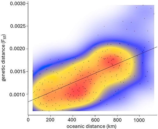
IBD based on pairwise comparisons of FST (estimated with neutral SNPs) and oceanic distances between all sampled statistical rectangles.
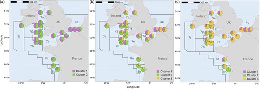
Pie charts based on admixture coefficient of individual sole as inferred by R package LEA at (a) K = 2 and (b) K = 3 using the neutral SNP dataset and (c) K = 3 using the outlier SNP dataset.
Pairwise fixation index (FST) values for putative sole groups based on ICES statistical rectangles and neutral SNPs after 10 000 bootstraps.
| NOS | EEC | WEC | CEL | IRE | BISC | |||||||||||||||||
|---|---|---|---|---|---|---|---|---|---|---|---|---|---|---|---|---|---|---|---|---|---|---|
| 4c | 4c | 4c | 7d | 7d | 7d | 7e | 7e | 7h | 7h | 7g | 7g | 7g | 7f | 7f | 7a | 7a | 7a | 8a | 8b | 8b | ||
| 31F1 | 31F2 | 31F3 | 29F0 | 30E9 | 28E9 | 29E7 | 28E3 | 27E3 | 27E4 | 32E3 | 32E4 | 30E3 | 29E4 | 30E4 | 36E6 | 36E4 | 33E4 | 22E7 | 19E8 | 20E7 | ||
| 4c | 31F2 | 0.0007 | ||||||||||||||||||||
| 4c | 31F3 | 0.0003 | 0.0002 | |||||||||||||||||||
| 7d | 29F0 | 0 | 0 | 0 | ||||||||||||||||||
| 7d | 30E9 | 0.0003 | 0.0006 | 0.0004 | 0 | |||||||||||||||||
| 7d | 28E9 | 0.0009* | 0.0009* | 0.0003 | 0 | 0 | ||||||||||||||||
| 7e | 29E7 | 0.0007 | 0.0006 | 0.0003 | 0 | 0 | 0 | |||||||||||||||
| 7e | 28E3 | 0.0016* | 0.0016* | 0.0017* | 0 | 0.0010 | 0.0006 | 0.0010 | ||||||||||||||
| 7h | 27E3 | 0.0014* | 0.0014* | 0.0009* | 0 | 0.0012* | 0.0007 | 0.0006 | 0 | |||||||||||||
| 7h | 27E4 | 0.0017 | 0.0024* | 0.0020* | 0 | 0.0010 | 0.0010 | 0.0010 | 0.0013 | 0 | ||||||||||||
| 7g | 32E3 | 0.0011* | 0.0012* | 0.0008 | 0 | 0.0010* | 0.0004 | 0.0007 | 0.0002 | 0 | 0 | |||||||||||
| 7g | 32E4 | 0.0015* | 0.0016* | 0.0010 | 0 | 0.0008 | 0.0010 | 0.0006 | 0.0003 | 0 | 0.0007 | 0 | ||||||||||
| 7g | 30E3 | 0.0017* | 0.0015* | 0.0013 | 0 | 0.0010 | 0.0003 | 0.0004 | 0 | 0 | 0.0008 | 0 | 0.0003 | |||||||||
| 7f | 29E4 | 0.0015* | 0.0014* | 0.0008* | 0 | 0.0014* | 0.0006 | 0.0009 | 0.0005 | 0 | 0.0011 | 0.0002 | 0.0003 | 0 | ||||||||
| 7f | 30E4 | 0.0015 | 0.0011 | 0.0017 | 0 | 0.0016 | 0.0003 | 0.0008 | 0.0009 | 0 | 0.0011 | 0 | 0 | 0 | 0.0004 | |||||||
| 7a | 36E6 | 0.0005 | 0.0006 | 0.0002 | 0 | 0 | 0.0008 | 0.0005 | 0.0005 | 0.0007 | 0.0011 | 0.0006 | 0.0004 | 0.0005 | 0.0005 | 0.0004 | ||||||
| 7a | 36E4 | 0.0009 | 0.0014* | 0.0007 | 0 | 0.0005 | 0.0007 | 0.0005 | 0.0003 | 0.0003 | 0.0002 | 0.0005 | 0.0002 | 0.0002 | 0.0004 | 0.0002 | 0 | |||||
| 7a | 33E4 | 0.0013* | 0.0015* | 0.0011* | 0 | 0.0009 | 0.0009 | 0.0007 | 0.0004 | 0.0004 | 0.0010 | 0.0007 | 0.0005 | 0 | 0.0004 | 0.0003 | 0.0004 | 0.0003 | ||||
| 8a | 22E7 | 0.0024* | 0.0025* | 0.0022* | 0 | 0.0017* | 0.0012* | 0.0014* | 0.0016* | 0.0009* | 0.0016 | 0.0013* | 0.0012* | 0.0012* | 0.0015* | 0.0008 | 0.0013* | 0.0017* | 0.0017* | |||
| 8b | 19E8 | 0.0028* | 0.0027* | 0.0027* | 0.0006 | 0.0022* | 0.0016* | 0.0018* | 0.0023* | 0.0015* | 0.0018* | 0.0019* | 0.0016* | 0.0015* | 0.0015* | 0.0012 | 0.0020* | 0.0017* | 0.0020* | 0.0008 | ||
| 8b | 20E7 | 0.0029* | 0.0025* | 0.0020* | 0 | 0.0016* | 0.0011* | 0.0013* | 0.0018* | 0.0006 | 0.0013 | 0.0010* | 0.0015* | 0.0004 | 0.0010* | 0.0004 | 0.0016* | 0.0016* | 0.0015* | 0.0001 | 0.0002 | |
| 7J | 32E0 | 0.0018* | 0.0019* | 0.0013* | 0.0001 | 0.0013* | 0.0007 | 0.0008* | 0.0014* | 0.0005 | 0.0015* | 0.0003 | 0.0008 | 0.0009* | 0.0005 | 0.0012 | 0.0011* | 0.0010* | 0.0010* | 0.0012* | 0.0015* | 0.0011* |
P-values < .01 are indicated with an asterisk (*)
Outlier SNPs dataset
Pairwise FST values estimated with outlier SNPs ranged from 0 to 0.1607, with the highest level of adaptive genetic differentiation between sole from the Bay of Biscay (8b) and the southern Celtic Sea (7h, statistical rectangle 27E4) (Table 5). Sole from the Bay of Biscay (8b, statistical rectangle 19E8) was significantly differentiated from all other statistical rectangles, including those within the Bay of Biscay (20E7 in 8b and 22E7 in 8a). Two ICES areas showed distinct adaptive divergence: the southern North Sea (4c, continental versus UK coast) and the Bay of Biscay (8b). Admixture analysis revealed three distinct clusters (K = 3) (Fig. 4c). Sole from the southernmost sampling location in the Bay of Biscay were predominantly assigned to cluster 2, while those collected near the Belgian coast in the southern North Sea were predominantly assigned to cluster 1. The population sub-structuring detected in the southern North Sea based on outlier SNPs could also be observed in the admixture analysis with the population near the UK mostly being assigned to cluster 3, while the populations near the Belgian coast were predominantly assigned to cluster 1. Sole from the English Channel and Celtic Seas were predominantly assigned to cluster 3.
Pairwise fixation index (FST) values for putative sole groups based on ICES statistical rectangles and outlier SNPs after 10 000 bootstraps.
| NOS | EEC | WEC | CEL | IRE | BISC | |||||||||||||||||
|---|---|---|---|---|---|---|---|---|---|---|---|---|---|---|---|---|---|---|---|---|---|---|
| 4c | 4c | 4c | 7d | 7d | 7d | 7e | 7e | 7h | 7h | 7g | 7g | 7g | 7f | 7f | 7a | 7a | 7a | 8a | 8b | 8b | ||
| 31F1 | 31F2 | 31F3 | 29F0 | 30E9 | 28E9 | 29E7 | 28E3 | 27E3 | 27E4 | 32E3 | 32E4 | 30E3 | 29E4 | 30E4 | 36E6 | 36E4 | 33E4 | 22E7 | 19E8 | 20E7 | ||
| 4c | 31F2 | 0.0350 | ||||||||||||||||||||
| 4c | 31F3 | 0.0235* | 0 | |||||||||||||||||||
| 7d | 29F0 | 0 | 0.0107 | 0.0011 | ||||||||||||||||||
| 7d | 30E9 | 0.0050 | 0 | 0 | 0 | |||||||||||||||||
| 7d | 28E9 | 0.0067 | 0.0246* | 0.0185 | 0 | 0.0059 | ||||||||||||||||
| 7e | 29E7 | 0.0059 | 0.0135 | 0.0036 | 0 | 0 | 0.0012 | |||||||||||||||
| 7e | 28E3 | 0.1107* | 0.0652* | 0.0543* | 0.0511 | 0.0726* | 0.0420 | 0.0598 | ||||||||||||||
| 7h | 27E3 | 0.0700* | 0.0424* | 0.0321* | 0.0299 | 0.0393 | 0.0202 | 0.0332 | 0 | |||||||||||||
| 7h | 27E4 | 0.0930* | 0.0789* | 0.0762* | 0.0371 | 0.0728* | 0.0411 | 0.0678 | 0.0419 | 0.0192 | ||||||||||||
| 7g | 32E3 | 0.0861* | 0.0854* | 0.0724* | 0.0407 | 0.0667* | 0.0326 | 0.0600* | 0.0121 | 0.0047 | 0.0071 | |||||||||||
| 7g | 32E4 | 0.0802* | 0.0514 | 0.0353* | 0.0264 | 0.0442 | 0.0299 | 0.0366 | 0 | 0 | 0.0238 | 0.0014 | ||||||||||
| 7g | 30E3 | 0.0827* | 0.0459 | 0.0364 | 0.0383 | 0.0509* | 0.0248 | 0.0428 | 0 | 0 | 0.0392 | 0.0132 | 0 | |||||||||
| 7f | 29E4 | 0.1080* | 0.0731* | 0.0624* | 0.0671 | 0.0836* | 0.0469* | 0.0750* | 0 | 0.0031 | 0.0229 | 0.0080 | 0.0038 | 0.0041 | ||||||||
| 7f | 30E4 | 0.0802 | 0.0437 | 0.0294 | 0.0424 | 0.0469 | 0.0345 | 0.0436 | 0 | 0 | 0.0220 | 0.0014 | 0 | 0 | 0 | |||||||
| 7a | 36E6 | 0.0155 | 0 | 0 | 0 | 0 | 0.0019 | 0 | 0.0381 | 0.0222 | 0.0627* | 0.0549* | 0.0258 | 0.0263 | 0.0550* | 0.0159 | ||||||
| 7a | 36E4 | 0.0331 | 0.0264 | 0.0149 | 0 | 0.0162 | 0.0028 | 0.0061 | 0.0171 | 0.0025 | 0.0445 | 0.0268 | 0.0121 | 0.0155 | 0.0292 | 0.0067 | 0.0088 | |||||
| 7a | 33E4 | 0.0437* | 0.0530* | 0.0447* | 0.0071 | 0.0290 | 0.0092 | 0.0271 | 0.0329 | 0.0088 | 0.0082 | 0 | 0.0088 | 0.0165 | 0.0281* | 0.0130 | 0.0279 | 0.0155 | ||||
| 8a | 22E7 | 0.0841* | 0.0469 | 0.0436* | 0.0408 | 0.0605* | 0.0442* | 0.0489* | 0.0361 | 0.0315 | 0.0761* | 0.0689* | 0.0346 | 0.0318 | 0.0467* | 0.0323 | 0.0393 | 0.0366 | 0.0516* | |||
| 8b | 19E8 | 0.1543* | 0.0944* | 0.1040* | 0.1105* | 0.1128* | 0.1103* | 0.1029* | 0.0853* | 0.0942* | 0.1607* | 0.1405* | 0.0933* | 0.0908* | 0.1075* | 0.0795* | 0.0984* | 0.0964* | 0.1255* | 0.0410* | ||
| 8b | 20E7 | 0.1046* | 0.0764* | 0.0760* | 0.0624 | 0.0842* | 0.0675* | 0.0682 | 0.0558 | 0.0551 | 0.0942* | 0.0866* | 0.0523 | 0.0466 | 0.0629* | 0.0501 | 0.0693 | 0.0609 | 0.0649* | 0 | 0.0379* | |
| 7J | 32E0 | 0.0708* | 0.0606* | 0.0466* | 0.0237 | 0.0458* | 0.0182 | 0.0303* | 0.0127 | 0.0034 | 0.0510* | 0.0168 | 0.0096 | 0.0152 | 0.0273 | 0.0230 | 0.0394 | 0 | 0.0154* | 0.0471 | 0.1023* | 0.0706 |
P-values < .01 are indicated with an asterisk (*).
Identification of candidate genes under selection
A Manhattan plot showed the physical distribution of the 76 outlier SNPs across chromosomes 1 to 21 on the sole reference genome (Fig. 5), indicating a genome-wide pattern of SNP distribution. A total of 59 out of 76 outlier SNPs were located in the coding region of a gene, and a total of 35 unique potential candidate genes were identified (Table S3). In several cases, multiple SNPs were detected in the coding region of the same candidate gene with a maximum of 5 SNPs detected in the lamb21 gene on chromosome 11, which is an immune-related gene.
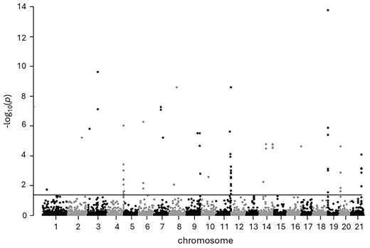
Manhattan plot of neutral and outlier SNPs (above threshold) and their respective positions on chromosomes 1 to 21 of the sole genome. The horizontal line indicates the genome-wide significance threshold (q-value = 0.05).
Variation in length and weight across areas
Sole showed variability in length across the different areas, with specimens caught in the Western English Channel (7e) and Celtic Seas area (7f and 7h) significantly larger than sole from other areas (P < .05), with the exception of 7f compared to Bay of Biscay (8a and 8b) and 7e compared to 8a (Fig. 6; Fig. S5; Table S4). Significant differences in weight were found between 7h and all other areas except for 7e, 7f, and southwest of Ireland (7j) (P < .05), for 7e and 7j with areas 4c, 7d, 7g, and 8b (P < .05), and between 7f and 7g (P < .05) (Fig. 6; Fig. S5; Table S4).
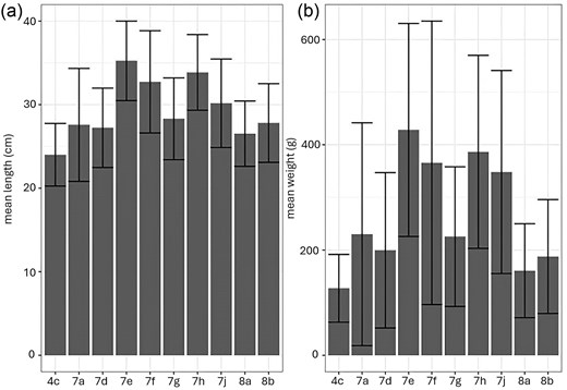
Barplot (± standard deviation) showing (a) mean length (cm) and (b) mean weight (g) of sampled sole per ICES area. Significant differences are indicated in the text and Table S4.
Discussion
Identifying the population structure and adaptive diversity of commercial fish species is crucial for effective and sustainable fisheries management (Pearse 2016). We revealed novel insights in the population structure of data-poor sole stocks in the southern Celtic Sea (7h) and southwest of Ireland (7j). We found no significant genetic differentiation between sole populations within the Celtic Sea (7f, 7g, and 7h) using both neutral and putative outlier loci. However, subtle population structuring of sole in the southwest of Ireland (7j) with several subpopulations in areas 7h (both neutral and outlier loci) and 7f (neutral loci) was observed. In addition, we did not detect significant genetic neutral differentiation between sole from the Celtic Sea (7f, 7g, and 7h) and the Irish Sea (7a), which provides evidence for the suggested Irish/Celtic Sea population in previous studies (Cuveliers et al. 2012, Diopere et al. 2018), and the Western English Channel (7e). The lack of genetic structure within these regions is corroborated by length and weight analyses obtained from the sampled sole, which showed no significant differences between the southern Celtic Sea (7h), Western English Channel (7e), and Celtic Sea (7f). These new findings are imperative information for sustainable fisheries management in these currently data-poor, yet commercially important fishing areas.
Sole in the Celtic Sea are genetically homogeneous
Our results reveal the presence of one genetically homogeneous sole population in the Celtic Sea (7f, 7g, and 7h). Furthermore, no neutral genetic differentiation was observed between sole from the Celtic Sea and sole from the Western English Channel (7e). Previous tagging experiments have suggested a counter-clockwise flux of plaice around the southern UK (Dunn and Pawson 2002), and similar pathways for sole could explain the connectivity between sole in the Western English Channel (7e) and Celtic Sea (7f, 7g, and 7h). In addition, no genetic differentiation was found between sole from the Western and Eastern English Channel (7e and 7d), providing additional evidence for the connectivity along the UK coasts. Moreover, sole from the Celtic Sea (7f, 7g, 7h) showed no significant differentiation with sole from the Irish Sea (7a). In the Irish Sea, eggs and larvae have been documented to disperse up to 300 km (van der Molen et al. 2007), yet prevailing winds and regional currents largely hamper the transport from east to west (Fox et al. 2009). In the case of another flatfish species, plaice, the majority of larvae originating from spawning grounds in the Eastern Irish Sea settled on nursery grounds along the Welsh, English, and Scottish coasts (Fox et al. 2009). Similar mechanisms can be expected for sole and could explain the lack of genetic differentiation observed in the Celtic Sea (7f, 7g, and 7h) and Irish Sea (7a). At the same time, the limited larval connectivity from those areas to the coast of Ireland could explain the observed genetic differentiation with the southern Ireland sole (7j). The connectivity between sole in the southwest of Ireland (7j) to the Irish Sea (7a) and, to some extent, other areas in the Celtic Sea appears to be limited. Simulations of current-mediated larval dispersal in cockles have shown that larvae released from coastal locations in southern Ireland are predominantly entrained in westward currents around southern Ireland, restricting the potential of larval connectivity from southern Ireland to other areas (Coscia et al. 2020). Moreover, there is no documented evidence of spawning or feeding migrations of sole from southern Ireland to areas in the Celtic Sea or Irish Sea.
Genetic differentiation between sole populations in the North-East Atlantic is low
Overall, sole showed low levels of genetic differentiation between putative populations within the North-East Atlantic with the highest level of genetic differentiation between sole from the Bay of Biscay (ICES areas 8a, 8b) and southern North Sea (4c), which is in agreement with previous studies (Exadactylos et al. 1998, Cuveliers et al. 2012, Diopere et al. 2018). These low levels of genetic differentiation could be explained by extensive larval dispersal between spawning and nursery grounds. Pelagic larval stages increase the opportunity for long-distance dispersal and are often associated with low levels of genetic differentiation over larger geographical distances (Riginos and Victor 2001). The dispersal distance of sole larvae shows the ability to link spawning and nursery grounds and is directly related to the time spent in the water column and hydro-dynamical conditions (Barbut et al. 2019). Larval exchanges between the southern North Sea (4c) and Eastern English Channel (7d) can occur in both directions, whereas the Western English Channel (7e) also receives larvae from the Eastern English Channel (7d), but usually not the other way around (Savina et al. 2016). This larval connectivity might explain the absence of neutral genetic differentiation between sole populations in the southern North Sea (4c) and Eastern English Channel (7d) and eastern English Channel (7d) and Western English Channel (7e). The Bay of Biscay does not generally receive larvae from other areas, and the proportion of larvae from the Bay of Biscay settling in the Western English Channel is low (± 2%) (Savina et al. 2016). Overall, while eggs and planktonic larval stages can clearly contribute to long-distance connectivity, oceanographic conditions and larval behaviour can favour certain pathways contributing to population structuring (Champalbert and Koutsikopoulos 1995, Riginos et al. 2011).
A second potential explanation for the low degree of genetic differentiation observed between populations is the migratory behaviour of juvenile and adult sole between feeding and spawning grounds. Selective tidal transport, a dispersal mechanism from feeding to spawning grounds (and the other way around) using tidal currents, likely plays an important role (Walker et al. 1980). Here, we list three well-documented migratory routes of adult flatfish using tidal transport to highlight the connectivity between several areas, which might explain the absence of genetic differentiation between the regions: (1) sole and plaice from feeding grounds in the Southern Bight of the North Sea (4c) to spawning grounds in the Eastern English Channel (7d) and vice versa (Walker and Emerson 1990, Metcalfe et al. 2006); (2) plaice from feeding grounds in the south-east Irish Sea (7a) to spawning grounds in the Bristol Channel (7f) and off south-east Ireland (7g) (Dunn and Pawson 2002); (3) plaice from feeding grounds in the Bristol Channel (7f) to spawning grounds in the Western English Channel (7e) (Dunn and Pawson 2002). Migratory routes undertaken by plaice are expected to be similar for sole. The connectivity of sole between the Bay of Biscay and other areas is rather limited, but movement into the Western English Channel has been observed (Koutsikopoulos et al. 1995). Here, significant differentiation between sole sampled in the Bay of Biscay (8a, 8b) and Western English Channel (7e) was observed. Interestingly, no genetic differentiation was found between sole from the Bay of Biscay and those from several sampling locations in the Celtic Sea (7f, 7g, and 7h) indicating some level of connectivity between the regions. Regardless, a pattern of IBD was observed, especially between the southern North Sea (4c) and Bay of Biscay (8a, 8b), highlighting the limits to overcome large-scale geographic distances. A similar pattern of IBD along the continental shoreline has also been observed for sole by Cuveliers et al. (2012) and Diopere et al. (2018).
The combination of high gene flow among populations in the North-East Atlantic, large effective population sizes, and the relatively young age of the marine habitat might explain the low levels of genetic differentiation based on neutral SNP markers (Cano et al. 2008). Glacial retreat at the end of the last ice age allowed the re-colonisation of the European seas by marine organisms. Potential isolation between populations can stay unnoticed for a long period as differences in allele frequencies will only slowly accumulate (Hauser and Carvalho 2008). In this study, the observed similarities between sole in the Irish Sea (7a) and the southern North Sea (4c) potentially reflect signatures of re-colonization after the last ice age. Similar hypotheses have been formulated for other high gene flow flatfish species like European plaice (Le Moan et al. 2021, Weist et al. 2022).
Patterns in adaptive variation suggest local adaptation
Despite high levels of gene flow and low levels of genetic population structuring commonly found in marine fishes, adaptive population divergence might be more prevalent than previously assumed (Nielsen et al. 2009, Limborg et al. 2012), including in local sole populations. For example, adaptive divergence was observed in the southern North Sea between sole sampled near the UK and Belgian coast. Furthermore, adaptive divergence was detected between sole from the southern North Sea (4c) and Eastern English Channel (statistical rectangle 30E9 near Newhaven, UK), and sole from the western sampling location in the Western English Channel but not the eastern part of the Western English Channel (7e). This adaptive divergence was not observed within the Western English Channel, although it became significant when a less stringent threshold (P = .05 instead of P = .01) was applied. These results suggest the presence of adaptive processes in the region, which require further research. Sole in the Bay of Biscay are generally considered to form a panmictic population (Cuveliers et al. 2012, Diopere et al. 2018), although spatial structuring between a southern and a northern group in the Bay of Biscay, at least on the nursery grounds, has been reported before (Guinand et al. 2008). While this study found no neutral genetic population structuring between the northern and southern components, adaptive genetic differentiation was detected between sole collected in two statistical rectangles in 8b and between the northern and southern parts of the Bay of Biscay. These findings are in agreement with several previous studies that have suggested different selective pressures acting on sole (Rolland et al. 2007, Guinand et al. 2008) and flounder (Marchand et al. 2003) in the Bay of Biscay.
Putative candidate genes underlying adaptive potential of sole populations
In this study, a total of 59 outlier SNPs were detected in 35 potential candidate genes spread across the sole genome. To highlight a few, five SNPs and two SNPs were detected in the laminin subunit beta 1 (lamb2l) and laminin subunit 2 (lamb2) gene region, which are immune-related genes previously identified in the spleen of the flatfish turbot Scophthalmus maximus (Song et al. 2024). A total of three and two SNPs were detected in the low-density lipoprotein receptor-related protein 2b (lrp2b) and very low-density lipoprotein receptor (vldlr) genes, respectively, both play an essential role in lipid metabolism (e.g. cellular signal transduction, cholesterol homeostasis, fatty acid uptake) (Cao et al. 2023). Two SNPs were detected in the collagen alpha-1 (X) chain gene, which is part of the collagen family that functions as important structural protein in connective tissues. In Atlantic salmon, collagen genes might be involved in the immune response to cope with sea lice and other diseases (López et al. 2019). Several other putative candidate genes (e.g. ST3GAL1) might also be related to immune responses (Decloquement et al. 2023), while others might be related to coloration (e.g. ATP-binding cassette sub-family G) (Feng et al. 2015). Diopere et al. (2013) previously identified 29 validated SNPs in eight candidate genes related to maturation and growth, but we did not detect SNPs in those candidate gene regions. Furthermore, we also did not detect the 19 outlier SNPs previously described in Diopere et al. (2018). However, similar to Diopere et al. (2018), several SNPs were detected in potential candidate genes related to muscle activity (i.e. Rho GTPase activating protein 42a, glycogen phosphorylase, SH3, and cysteine-rich domain-containing protein 3-like). Our findings clearly require further research, as adaptive population divergence has important implications for the management and conservation of sole under rapidly increasing evolutionary pressures from fisheries- and climate-induced changes, especially on a local scale.
Revision of current stock units for sustainable fisheries management
Stocks have been traditionally managed according to geographical boundaries, in European waters typically according to ICES divisions. Biological stocks, however, are more complex and dynamic, which could result in potential mismatches between traditional management areas and biological stocks (Reiss et al. 2009). A mismatch between the managed stock and the effective biological population can lead to the overexploitation of some spawning components and ultimately, the entire biological population (Abaunza et al. 2008). Currently, sole in our study area is managed according to the following seven ICES stocks: 7f and 7g (Celtic Sea), 7a (Irish Sea), 7hjk (southern Celtic Sea South and southwest of Ireland), 4 (North Sea), 7d (Eastern English Channel), 7e (Western English Channel), and Bay of Biscay (8a and 8b). Sole populations in ICES areas 7h, 7f, and 7g were genetically similar on both a neutral and adaptive level. Despite the lack of neutral genetic differentiation among sole in the Celtic Sea (7f, 7g, 7h), Irish Sea (7a), and Western English Channel (7e), significant population differentiation between several statistical rectangles in these areas in the outlier dataset highlights the role of local adaptation. Although our sampling in the southwest of Ireland (7j) was limited to one location, the sample size and number of SNPs included in our analyses provided strong support for the genetic signal observed in these samples. Sole from the southwest of Ireland (7j) were significantly differentiated from all other ICES areas, with the exception of sole in the Celtic Sea (7f), which suggests at least some connectivity between the southwest of Ireland and the Celtic Sea. On the statistical rectangle level, sole from area 7j was significantly differentiated with sole from one rectangle in area 7h (neutral and outlier loci) and 7g (neutral loci). Based on our genetic data, we conclude that sole from 7h and 7j should not form one stock. Instead, sole from southwest of Ireland (7j) could be considered as one management unit, and sole from southwest of the Celtic Sea (7h) could form one management unit together with sole from 7f and 7g. Yet, biological data must be taken into consideration as well. For instance, sole from area 7g were significantly smaller and weighted less compared to sole collected in 7e, 7f, and 7h, which is likely related to the larger proportion of younger fish sampled in that area. Therefore, analysing differences in growth patterns with a more comprehensive dataset could clarify this.
Conclusion
This study revealed several novel insights into the population structure of sole in the Celtic Seas, including the stock identity of sole in two data-poor regions: the southern Celtic Sea (7h) and southwest of Ireland (7j). We propose a revision of the current stock status of 7hjk and recommend the establishment of two distinct management units: sole from the southwest of the Celtic Sea (7h) combined with sole from 7fg and sole from the southwest of the of Ireland (7j).The lack of genetic structure between the southern Celtic Sea (7h) and Celtic Sea (7f) is supported by biological metadata related to length and weight. In addition, multiple potential candidate genes have been identified, which can be used for investigating signatures of selection in future research. Our genetic findings in combination with biological parameters are imperative to inform stock assessments to ensure the implementation of sustainable fisheries management.
Acknowledgements
Research was conducted under the project SoleDNA funded by the European Maritime and Fisheries Fund (EFMZV) and the Financial Instrument for the Flemish Fisheries and Aquaculture Sector (FIVA). We are very grateful for everyone that helped collect sole samples. We would like to thank Laurence Desmet from ILVO for help with laboratory preparations. We would also like to express our gratitude to Claire Moore from the Irish Marine Institute for providing sole samples from Irish waters. At last, we would like to thank Prof. Filip Volckaert and Enora Geslain from KU Leuven for sharing the reference genome of sole.
Author contributions
Sarah M. Maes (Data curation [lead], Formal analysis [lead], Project administration [supporting], Writing – original draft [lead], Writing – review & editing [lead]), Lies Vansteenbrugge (Conceptualization [equal], Data curation [supporting], Formal analysis [supporting], Funding acquisition [equal], Project administration [equal], Writing – original draft [supporting], Writing – review & editing [supporting]), Margo Van Canneyt (Data curation [equal], Formal analysis [supporting], Writing – original draft [supporting], Writing – review & editing [supporting]), Tom Ruttink (Data curation [supporting], Formal analysis [supporting], Writing – original draft [supporting], Writing – review & editing [supporting]), Els Torreele (Conceptualization [equal], Funding acquisition [equal], Project administration [supporting], Writing – original draft [supporting], Writing – review & editing [supporting]), and Sofie Derycke (Conceptualization [equal], Data curation [supporting], Formal analysis [supporting], Funding acquisition [equal], Project administration [equal], Writing – original draft [supporting], Writing – review & editing [supporting])
Conflict of interest
The authors have no conflicts of interest to declare.
Funding
Research was conducted under the project SoleDNA funded by the European Maritime and Fisheries Fund (EFMZV) and the Financial Instrument for the Flemish Fisheries and Aquaculture Sector (FIVA).
Data availability
The raw sequence reads generated in this study have been deposited in the Sequence Read Archive (SRA) under the accession number PRJNA1229163 and can be accessed at https://www.ncbi.nlm.nih.gov/sra/PRJNA1229163. The data and R scripts used for the analyses are available in Zenodo at 10.5281/zenodo.14988907.
