


Abstract
Antarctic krill (Euphausia superba) and Ice krill (Euphausia crystallorophias) are key species within Southern Ocean marine ecosystems. Given their importance in regional food webs, coupled with the uncertain impacts of climate change, the on-going recovery of krill-eating marine mammals, and the expanding commercial fishery for Antarctic krill, there is an increasing need to improve current estimates of their circumpolar habitat distribution. Here, we provide an estimate of the austral summer circumpolar habitat distribution of both species using an ensemble of habitat models and updated environmental covariates. Our models were able to resolve the segregated habitats of both species. We find that extensive potential habitat for Antarctic krill is mainly situated in the open ocean and concentrated in the Atlantic sector of the Southern Ocean, while Ice krill habitat was concentrated more evenly around the continent, largely over the continental shelf. Ice krill habitat was mainly predicted by surface oxygen concentration and water column temperature, while Antarctic krill was additionally characterized by mixed layer depth, distance to the continental shelf edge, and surface salinity. Our results further improve understanding about these key species, helping inform sustainable circumpolar management practices.
Introduction
Antarctic krill (Euphausia superba) and Ice (or crystal) krill (Euphausia crystallorophias) are both key ecological species in the Southern Ocean (Murphy et al., 2012; Murphy et al., 2016). They are important prey for many marine top predators (Meyer et al., 2020) and invertebrates (Trathan and Hill, 2016), as well as being important grazers of autotrophic and heterotrophic plankton (Bar-On et al., 2018). Both species are essential in energy flow (Ballerini et al., 2014) and nutrient cycling (Ratnarajah and Bowie, 2016) through their high biomass and daily vertical migration, transporting essential nutrients and stimulating primary productivity (Cavan et al., 2019).
Antarctic krill is more abundant and ecologically important in mid- to lower-latitudes, including around some sub-Antarctic islands, especially in the southwest Atlantic (e.g. Murphy et al., 2016). In contrast, Ice krill is more abundant and ecologically important in high-latitude coastal zones, including coastal polynyas (Pakhomov, 1997), where it is often the principal food source for many coastal top predators (Thomas and Green, 1988; La et al., 2015). Both krill species have a complex life cycle closely associated with the winter sea ice (Pakhomov, 1997; Meyer et al., 2017) and a lifespan up to six years (Siegel, 1987). Spawning takes place during late spring (Pakhomov, 1997) and from spring to late summer (Spiridonov, 1995; Siegel, 2005) for Ice krill and Antarctic krill, respectively. Thus, krill distribution in the Southern Ocean is a function of time and space. Information on the potential habitats of both species is therefore of importance to a range of stakeholders. These include ecological modellers aiming to develop models incorporating the full spatiotemporal life history of krill (Thorpe et al., 2019; Green et al., 2021), ecologists trying to better understand circumpolar recruitment and connectivity (Meyer et al., 2020), and for the on-going management and policy development towards holistic spatial management approaches (McCormack et al., 2021).
Antarctic krill is the focus of a modern fishery (Hill et al., 2016; Trathan et al., 2018; Trathan et al., 2021; Trathan et al., 2022a; Trathan et al., 2022b) managed by the Commission for the Conservation of Antarctic Marine Living Resources (CCAMLR). There is currently no commercial fishery targeting Ice krill. Within CCAMLR, efforts to develop coherent spatial management have been underway for nearly two decades (Brooks et al., 2020; Trathan and Grant, 2020). Knowledge about favourable habitats is essential to the development of spatial planning solutions that aim to conserve biodiversity, minimize risk associated with climate change, and help retain species both now and into the future (Eyring et al., 2021). Recent efforts have focused on developing new approaches to “future proof” krill spatial management for climate change (Arafeh-Dalmau et al., 2021) and climate-smart conservation planning (Tittensor et al., 2019). These types of approaches require a baseline of the current spatial distribution and factors determining the distribution of key ecological species, including Antarctic krill and Ice krill.
Historically, the main region of krill research with the most observational data have been the southwest Atlantic sector of the Southern Ocean (CCAMLR MPA Planning Domain 1, Figure 1; Atkinson et al., 2008; Atkinson et al., 2017), which is also the focus of the modern Antarctic krill fishery (Nicol and Foster, 2016). Observational data on Antarctic krill outside this region remains relatively scarce, while data on Ice krill is sparse throughout the Southern Ocean . Consequently, earlier studies focused on modelling specific aspects of present-day and projected krill habitat, mainly focusing on Antarctic krill. These include modelling habitat for enhanced growth using an empirical growth model (Hill et al., 2013; Murphy et al., 2017; Veytia et al., 2020) and identifying spawning habitat quality by simulating larval recruitment combined with a mechanistic model of spawning quality (Piñones and Fedorov, 2016; Thorpe et al., 2019; Green et al., 2021). Both approaches are based on observations in the southwest Atlantic sector and then upscaled to explore circumpolar distributions. Further, several studies used ecological niche theory (Guisan and Thuiller, 2005; Elith and Leathwick, 2009), describing the species’ fundamental niche using environmental factors as an approximation of the realized niche, to predict the species potential habitat (Cuzin-Roudy et al., 2014; Silk et al., 2016; Davis et al., 2017). Some projections suggest that favourable habitats for Antarctic krill might contract, resulting in southward habitat shifts and possible declines in abundance and/or biomass. The extent to which a shift has already occurred and the potential future effects remain a topic of debate and active research (Cox et al., 2018; Atkinson et al., 2019; Hill et al., 2019; Veytia et al., 2020). Recent work focusing on Antarctic krill habitat, abundance, and predator consumption at the West Antarctic Peninsula (WAP; Warwick-Evans et al., 2022a; Warwick-Evans et al., 2022b) and around the South Sandwich Islands (Baines et al., 2022) has led to proposals for revised fisheries management. Such regionally focused work highlights the need to consider wider issues, including the broad geographic scale of krill habitat, large-scale movement between areas, population connectivity, and the development of a stock hypothesis.
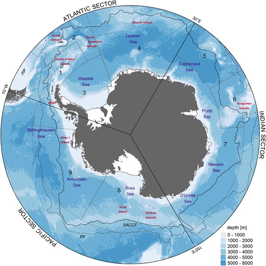
Map of the study area highlighting referenced locations throughout the text and the CCAMLR Marine Protected Area (MPA) Planning Domains (1–9) as stippled black lines. Seas are denoted in purple and island groups in red. Solid lines illustrate the common division of the Southern Ocean into the Atlantic, Indian, and Pacific sectors. Bathymetry (BATH) data displayed is IBCSO v2 (Dorschel et al., 2022). The Polar Front (PF) and Southern Antarctic Circumpolar Current Front (SACCF) are illustrated as stippled and solid black lines, respectively (Park et al., 2019). WAP - West Antarctic Peninsula. The Planning Domains are Domain 1: Western Peninsula - South Scotia Arc; Domain 2: North Scotia Arc; Domain 3: Weddell Sea; Domain 4: Bouvet Maud; Domain 5: Crozet - del Cano; Domain 6: Kerguelen Plateau; Domain 7: Eastern Antarctica; Domain 8: Ross Sea; and Domain 9: Amundsen - Bellingshausen.
Here, we use an ensemble of habitat suitability models (HSMs) based on observational data and observed environmental covariates to quantify the circumpolar summer habitat of Antarctic krill and Ice krill and better understand the drivers of the distribution of both species. We focus on the austral summer (December–March), the period of most observational data for both krill species, and the general time period when the adult krill population spawns, leading to future recruitment (Pakhomov, 1997; Siegel, 2005). Our modelling approach utilizes state-of-the-art statistical approaches as well as novel circumpolar environmental data products that characterize both the surface and subsurface conditions to evaluate the relative importance of different environmental factors and identify preferred habitats for each krill species. In a changing ocean, such information is increasingly vital for responsible management. Even though our models do not provide detailed biochemical or autecological perspectives for either species, they provide a description of the most important drivers of distribution, which may also be important when reviewing the evidence base supporting climate-smart decision-making related to spatial management (Tittensor et al., 2019).
Methods
Environmental covariates
The model domain for this study was the Southern Ocean south of 50°S, which encompasses much of the Antarctic Circumpolar Current (ACC), including two of its major fronts, the Polar Front (PF) and the Southern Antarctic Circumpolar Current Front (SACCF), and the subpolar waters to the south of the ACC (Park et al., 2019). It also contains at least parts of all nine CCAMLR MPA Planning Domains (Figure 1). These were created by CCAMLR to assist with on-going marine spatial planning projects and collectively cover the entire CCAMLR Convention Area (Penhale and Koubbi, 2011).
Krill potential habitat was modelled with an initial set of climatological means of 19 environmental variables, identified as potentially ecologically relevant to both species and influencing their abundance and spatial distribution (Table 1; Flores et al., 2008; Atkinson et al., 2009; Cuzin-Roudy et al., 2014; Duhamel et al., 2014; Silk et al., 2016; Bestley et al., 2018). We chose to use climatological means (integrated over 20–50 years) rather than annual information to describe the overall potential habitat rather than inter-annual variations, following Pinkerton et al. (2020). Further, insufficient information was available for most environmental covariates as well as krill observations to model inter-annual differences. Colinearity (i.e. when two or more variables described the same pattern) was assessed using the variance inflation factor metric in the “usdm” R package (Naimi et al., 2014) and a recommended threshold of 10 (Dormann et al., 2013). All variables were standardized (mean centred at 0 and standard deviation scaled to 1) before calculating colinearity (Naimi and Araújo, 2016). Surface dissolved oxygen concentration (SOX), sea surface temperature (SST), and temperature at 200 m depth (T200) showed high levels of colinearity (0.90–0.94 rp, Supplementary Figure S1). These covariates have been previously shown to be important to determine the habitat of both species (Brierley and Cox, 2010; Cuzin-Roudy et al., 2014; Tremblay and Abele, 2016; Murphy et al., 2017). Therefore, these three variables were combined to one latent variable using the first axis of a principal component analysis (PCA), explaining 95% of the initial variability (Supplementary Figure S2). The combination of testing for colinearity and the PCA reduction resulted in 12 environmental covariates as candidate habitat predictors (Table 1, Supplementary Figure S1). Grids for all variables were projected to a South Pole Lambert Azimuthal Equal Area projection (EPSG: 102020, Supplementary Figure S3) using bilinear interpolation at a 10 x 10 km resolution. All analyses were conducted in R 4.2.2 (R Development Core Team, 2022).
Environmental variables considered as habitat predictors.
| Environmental variable | Rationale | Source | Temporal coverage | Temporal resolution | Spatial resolution |
|---|---|---|---|---|---|
| Mean chlorophyll a (Chl a) concentration during the bloom season (BM) Bloom duration (BD) | Proxy for surface primary production in time and space (Racault et al., 2012) | Calculated from Ocean Colour—Climate Change Initiative (Sathyendranath et al., 2019) following Racault et al. (2012) | 1998–2019 | Annual climatology calculated from 8-d means | 9 km |
| Mean summer sea ice concentration (ICECONC) Mean summer sea ice persistence (ICEPERS)¤ | Proxy for habitat and prey availability (Lomakina, 1964; Meyer et al., 2020) | Sea ice trends and climatologies from SMMR and SSM/I-SSMIS, Version 3 (Stroeve and Meier, 2018) | 1978–2018 | Dec—Mar climatology calculated from monthly climatologies | 0.25° |
| Timing of spring sea ice retreat (ICEMELT) Duration of the sea ice-covered season (ICEDUR) ¤ Marginal ice zone (15–50% sea ice concentration) occurrence frequency during spring (MIZ) | Proxy for habitat and prey availability in space and time (Meyer et al., 2020) and important for krill swarm formation (Brierley and Cox, 2010) | Calculated from Sea Ice Concentrations from Nimbus-7 SMMR and DMSP SSM/I-SSMIS Passive Microwave Data, Version 1 (Cavalieri et al., 1996) following Stammerjohn et al. (2008) | 1978–2019 | Annual climatology calculated from alternately daily (pre-1987) or daily (starting 1987) data | 0.25° |
| Distance to coastal polynyas (ICEPOL) | Proxy for food availability for Ice krill (Pakhomov, 1997) | Calculated from average ice production following Nihashi and Ohshima (2015) | 2003–2010 | Annual average climatology | 6.25 km |
| Bathymetry (BATH) Distance to continental shelf edge (DIS, defined as 1000 m depth isobath) | Important for krill reproduction (Pakhomov and Perissinotto, 1996; Siegel and Watkins, 2016; Davis et al., 2017) | IBCSO v2 (Dorschel et al., 2022) | – | – | 500 m |
| Mixed layer depth (MLD) | Proxy of subsurface Chl a maxima as important food source for krill (Baldry et al., 2020) | (Pellichero et al., 2017) | 2002–2014 | Jan—Mar climatology | 0.5° |
| Sea surface silicate (SSI)¤ Sea surface nitrate (SSN)¤ | Proxy for primary production limitation (Boyd, 2002; Petrou et al., 2016) | World Ocean Atlas 2018 (Boyer et al., 2018) | 1955–2010 | Dec—Mar climatology calculated from monthly climatologies | 0.25° and 1° |
| Sea surface salinity (SSS) Sea surface temperature (SST)* | Proxy for Antarctic Surface Water (AASW), important for krill habitat selection (Cuzin-Roudy et al., 2014) and Antarctic krill reproduction (Atkinson et al., 2006) | ||||
| Surface dissolved oxygen concentration (SOX)* | Important for survival (Tremblay and Abele, 2016) and swarm formation (Brierley and Cox, 2010) | ||||
| Temperature at 200 m depth (T200)* Salinity at 200 m depth (S200) | Proxy for Circumpolar Deep Water (CDW), important during Antarctic krill early life cycle (Ross et al., 1988) |
covariates combined due to their high colinearity using PCA; ¤ removed prior to modelling due to high colinearity (Supplementary Figure S1) using the variable inflation factor metrics.
Krill occurrence data
Net and trawl data containing Antarctic krill and Ice krill information were collated from the most currently known expeditions within the study area (Fevolden, 1980; Makarov et al., 1985; Falk-Petersen et al., 1999; Fahrbach et al., 2003; Krafft et al., 2010; Swadling et al., 2010; Siegel, 2012; Atkinson et al., 2017; Steen, 2019; GBIF, 2020; Teschke et al., 2020 and references therein; Yang et al., 2021). Resulting datasets for each species were filtered to include: (1) spatial and temporal information (i.e. where and when collected); (2) only data on adults (i.e. removing juvenile and larvae data); (3) data after 1970 to correspond with the baseline period of habitat predictors (see Table 1); and (4) data collected during the austral summer (1 December–31 March). All available abundance data were transformed into presence-absence data. Absence observations were only retained with an upper sampling depth of <50 m and where >100 m of water column had been sampled to avoid false negatives (Atkinson et al., 2009). To reduce the spatial bias in sampling efforts, data were gridded at the resolution of the environmental covariates following Mormède et al. (2014). In cells with both presences and absences, only presences were retained. This way, the initial presence-absence datasets for Antarctic krill and Ice krill were reduced from 7975 and 1062 to 3222 and 479 observations, respectively (Figure 2d, Table 2).
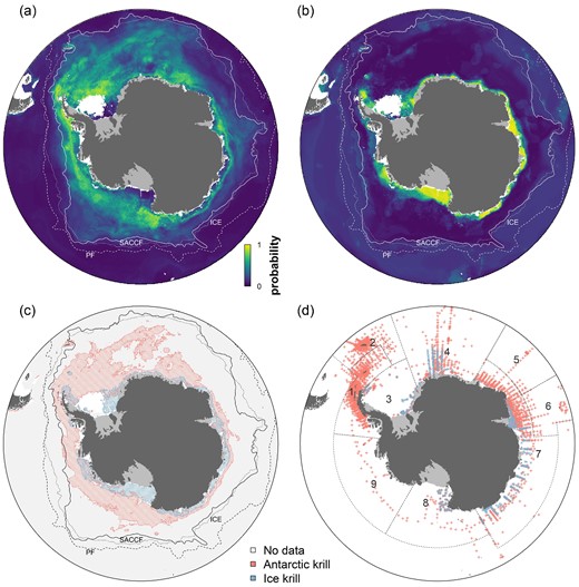
Habitat suitability estimates for (a) Antarctic krill (E. superba) and (b) Ice krill (E. crystallorophias). (c) Comparison of estimated habitat based on species-specific HSMs using 0.40 and 0.46 as binary cut-off maximizing the area under the receiver operating characteristic curve (AUC) for Antarctic krill and Ice krill, respectively. The PF, SACCF, and >10 d with sea ice coverage each year (ICE) are illustrated in (a–c) as stippled, solid black, and dotted lines, respectively (Park et al., 2019). (d) Observational data distribution (presences and absences) for the two species used to model species-specific HSM, including CCAMLR MPA Planning Domains 1–9.
Distribution of Antarctic krill (E. superba) and Ice krill (E. crystallorophias) observational data and ensemble model validation by CCAMLR MPA Planning Domains and across the entire model domain.
Species | CCAMLR MPA Planning Domains | Observational data | Spatial predictability | rs with IWC catch data | ||
|---|---|---|---|---|---|---|
| Presence | Absence | CBI | AUC | |||
| Antarctic krill | 1 | 997 | 299 | 0.99 | 0.82 | 0.68 |
| 2 | 169 | 251 | 0.86 | 0.78 | 0.39 | |
| 3 | 56 | 54 | 0.34 | 0.95 | 0.10 | |
| 4 | 182 | 144 | 0.98 | 0.82 | 0.16 | |
| 5 | 7 | 43 | 0.78 | 0.89 | 0.62 | |
| 6 | 21 | 73 | 0.83 | 0.91 | 0.83 | |
| 7 | 449 | 336 | 1.00 | 0.84 | 0.85 | |
| 8 | 37 | 56 | 0.81 | 0.90 | 0.76 | |
| 9 | 14 | 19 | 0.30 | 0.74 | 0.59 | |
| Southern Ocean | 1 972 | 1 250 | 1.00 | 0.85 | 0.58 | |
| Ice krill | 1 | 3 | 5 | 0.67 | 1.00 | – |
| 2 | 0 | 0 | – | – | – | |
| 3 | 42 | 34 | 0.90 | 0.96 | – | |
| 4 | 17 | 92 | 0.87 | 1.00 | – | |
| 5 | 0 | 0 | – | – | – | |
| 6 | 0 | 0 | – | – | – | |
| 7 | 137 | 102 | 0.76 | 0.99 | – | |
| 8 | 23 | 22 | 0.66 | 1.00 | – | |
| 9 | 0 | 0 | – | – | – | |
| Southern Ocean | 232 | 247 | 0.97 | 0.99 | – | |
AUC - area under the receiver operating characteristic curve; CBI - continuous Boyce index; rs - Spearman rank correlation; and IWC - International Whaling Commission.
Habitat suitability modelling
HSMs were built for both species using boosted regression trees with a binomial distribution and logit link (Mormède et al., 2014) following best practice (Elith et al., 2008). Each model was run using the biomod2 R package (Thuiller et al., 2009). For each boosted regression tree, a maximum number of 3000 trees were computed with an interaction depth of 5 and shrinkage of 0.01. Each species response dataset was modelled 10 times with 70% of the data randomly selected, with the remaining 30% of the data used to evaluate each model’s performance (i.e. cross validation). An ensemble model as a weighted average of all ten model runs was then calculated, using the model performance metric AUC to weigh each individual model run. AUC measures the ability of a model to distinguish between classes (Fielding and Bell, 1997; Lobo et al., 2008). In the case of HSMs, it indicates how well the model can discriminate between presence and absence observations. For AUC values close to 1, the classification is close to perfect; for values equal to 0.5, the model classification is no better than a random draw; and for values below 0.5, the model performs an inverse classification. That is, it predicts presences in areas dominated by absence points. The uncertainty of the habitat prediction was estimated using the coefficient of variation (CV), defined as the standard deviation divided by the mean of probabilities across all model runs. CV is a measure of uncertainty, with a high evaluation score denoting areas with high uncertainty. The lower the CV, the better the models are in that area. Relative importance of each predictor variable in each model was estimated using a permutation method, which randomly permutes each predictor variable independently, and computes the associated reduction in predictive performance (Thuiller et al., 2009). Habitat probability estimates were converted to species-specific binary maps by maximizing the AUC and thus determining a probability cutoff for each species-specific model. These were used to quantify species-specific habitat areas and the overlap between the two species.
Model validation
The HSM for each species was evaluated using cross-validation (as described above) and spatial predictability across the study area. To assess spatial predictability, the response data and model predictions were separated into the nine CCAMLR MPA Planning Domains (Figure 1). The ensemble model prediction was evaluated in each domain with available response data using the AUC and the continuous Boyce index (CBI). Boyce et al. (2002) suggested a performance indicator based on the relationship between the number of occurrences and the corresponding binned values of suitability (Hirzel et al., 2006). The relationship is measured by the Spearman rank correlation coefficient. A CBI value close to 1 suggests a close relationship between the number of occurrences and the predicted suitability, a value equal to 0 suggests no relationship, while a negative value suggests an inverse relationship. In contrast to AUC, CBI is independent of absence observations and was used here as a complementary approach to evaluate models both in terms of presence-absence (i.e. AUC) as well as presence-only information (i.e. CBI). We calculated CBI by applying the moving window method suggested by Hirzel et al. (2006) and using the ecospat R package (Broennimann, 2020).
The Antarctic krill HSM was tested against an independent dataset of historical whaling data assembled by the International Whaling Commission (IWC; Allison, 2020). For this validation, only catch data of krill-feeding species (blue whales Balaenoptera musculus, fin whales B. physalus, humpback whales Megaptera novaeangliae, and Antarctic minke whales B. bonaerensis) caught during the austral summer (December–March) 1902–2019 were considered. The resulting individual catch data were summed on a one-degree longitude-latitude grid across the model domain due to the low spatial resolution of pre-1973 data. These gridded data were then compared to the Antarctic krill HSM using the Spearman rank correlation coefficient across the model domain as well as within each CCAMLR MPA Planning Domain. Additionally, the Antarctic krill HSM was compared with pre-1960 occurrence data on Antarctic krill (December–March 1926–1951; Atkinson et al., 2017). The ensemble model for each species was tested using AUC and CBI across the entire model domain as well as within each CCAMLR MPA Planning Domain.
Results
The ensemble HSMs predicted circumpolar habitat suitability and associated uncertainty for both krill species (Figure 2 and Supplementary Figure S4). Antarctic krill habitat (estimated from HSM using a 0.40 binary cutoff maximizing the AUC) was concentrated in the Atlantic sector of the Southern Ocean (51% of predicted habitat, Figure 3 and Supplementary Figure S5), including the Weddell Sea, Lazarev Sea, western Antarctic Peninsula (WAP), and South Orkney Islands, and as far north as South Georgia, the South Sandwich Islands, and Bouvet Island (Figure 2). Suitable habitat is also predicted in the Indian sector (12%, Cosmonauts Sea and Prydz Bay, and to a lesser extent, Mawson Sea and D'Urville Sea), as well as the Pacific sector (36%, off the continental shelf in the Ross Sea as far north as the Balleny Islands, as well as in the Amundsen Sea and Bellingshausen Sea). Contrastingly, Ice krill habitat (estimated from HSM using a 0.46 binary cut-off maximizing the AUC) was more evenly predicted around the Antarctic continent (28–42% in each sector; Figure 3 and Supplementary Figure S5), with a more southern distribution compared to Antarctic krill habitat. Ice krill habitat was mainly predicted on the continental shelf and concentrated in the Ross Sea, Amundsen Sea, Weddell Sea, and Prydz Bay (Figures 2 and 3). Estimated habitat in the southern Weddell Sea was more uncertain, visible as higher estimated standard deviations across models runs (Supplementary Figure S4). A total area of 9.22 × 10⁶ km2 was estimated to be suitable habitat for both species within the model domain. Antarctic krill habitat area is predicted to be 8.14 × 10⁶ km2 (88% of total krill habitat), while Ice krill habitat area was predicted to be 2.01 × 10⁶ km2 (22% of total krill habitat). Species overlap was estimated to be 0.93 × 10⁶ km2 (10% of total krill habitat). Antarctic krill habitat was predominantly predicted in the open ocean (86% of its habitat) and, to a lesser extent, over the continental shelf. Contrastingly, Ice krill habitat occurred mainly over the continental shelf (72% of its habitat).
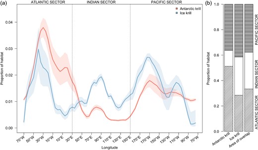
(a) Proportion of habitat estimated for Antarctic krill (E. superba) and Ice krill (E. crystallorophias) throughout the Southern Ocean, and (b) accumulated by ocean sector. Shadings in panel (a) illustrate variation of all 10 model runs for each species.
Environmental covariates most influential in predicting Antarctic krill habitat were mixed layer depth (MLD), distance to the continental shelf edge (DIS), the integrated measure of surface dissolved oxygen concentration, sea surface temperature, and temperature at depth (covariates combined using PCA), as well as sea surface salinity (SSS; Figure 4 and Supplementary Figure S6). Ice krill habitat was mainly predicted by the integrated variable of surface dissolved oxygen, surface temperature, and temperature at depth (PCA), and to a small degree by average bloom intensity (BM) and distance to the continental shelf edge (DIS).
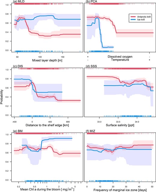
Marginal response plot of the six most influential variables (see Supplementary Figure S4, keeping all other variables at their median) for both species' ensemble models: (a) MLD; (b) latent variable of SST, temperature at 200 m, and sea surface dissolved oxygen concentration (PCA); (c) distance to the continental shelf edge (DIS); (d) SSS; (e) average bloom intensity (BM); (f) frequency of marginal sea ice zone (MIZ). Shaded areas illustrate the variability of the response across the 10 model runs. Rug plots at the top and bottom of each plot denote the observational data distribution for Antarctic krill (E. superba) and Ice krill (E. crystallorophias), respectively.
Cross-validation of each set of 10 HSM models for both species demonstrated good model fit with AUC values (measure of presence-absence fit) of 0.74 to 0.95 and 0.96 to 1.00 for Antarctic krill and Ice krill, respectively. The ensemble HSMs for either species also showed high performance measures throughout the model domain apart from some geographic areas with few observational data (Table 2). This was apparent in both AUC and CBI (measure of presence-only fit) values. Predicted Antarctic krill habitat was in general agreement with the independent IWC whale catch dataset (Table 2, Supplementary Figure S7) and early observational data collected between 1926 and 1951 (CBI = 0.82, AUC = 0.67, Supplementary Table S1).
Discussion
Circumpolar habitat distribution
We developed circumpolar summer habitat models for two key species of the Southern Ocean: Antarctic krill and Ice krill. Our estimates utilize observational data from across the Southern Ocean and are based on improved reanalyses of observational data and estimates of environmental covariates, the latter benefiting from recent data assimilation from research cruises, remote sensing, and the use of technology attached to marine mammals (Pellichero et al., 2017; Boyer et al., 2018; Dorschel et al., 2022). The resulting differential circumpolar distributions of the two species are in general agreement with previous, mainly regional, biogeographical studies (Mackintosh, 1973; Atkinson et al., 2009; Hill et al., 2013; Cuzin-Roudy et al., 2014; Piñones and Fedorov, 2016; Silk et al., 2016; Davis et al., 2017; Murphy et al., 2017; Thorpe et al., 2019; Veytia et al., 2020; Green et al., 2021; Yang et al., 2021; Baines et al., 2022; Warwick-Evans et al., 2022b). Agreement with previous studies, mainly focusing on Antarctic krill and using diverse approaches (e.g. growth model, spawning quality model, regional HSM), suggests that the overall habitat of both species is in part driven by large-scale environmental features such as frontal zones, the continental shelf break, and the winter sea ice extent, which delimit bioregions (Raymond, 2014; Park et al., 2019). The association between frontal zones and predicted species habitat has also been shown for other species groups, including marine mammals and seabirds (Hindell et al., 2020), mesopelagic fish (Freer et al., 2019), mesozooplankton (Pinkerton et al., 2020), and echinoid fauna (Fabri-Ruiz et al., 2020).
For Antarctic krill, we found that most habitat was predicted in the Atlantic Sector (Cuzin-Roudy et al., 2014), particularly in the southwest Atlantic sector (CCAMLR MPA Planning Domains 1 and 3) (Hill et al., 2013; Silk et al., 2016; Baines et al., 2022). Our results also suggest extensive potential habitat in the Lazarev Sea (CCAMLR Planning Domain 4), supporting previous work (Krafft et al., 2010). Further, we identified large areas of suitable habitat in the Indian and Pacific Sectors, especially in the Ross Sea (Davis et al., 2017) and the little-surveyed Amundsen and Bellingshausen Seas, including around Peter I Island (Atkinson et al., 2008). In contrast, we did not determine habitats within the deeper parts of the Southern Ocean in the northern Cosmonaut and Amundsen Seas, as previously described by Cuzin-Roudy et al. (2014). Overall, our model supports previous work predicting an extensive unequal circumpolar distribution of Antarctic krill, mainly off the continental shelf during summer (Mackintosh, 1973; Atkinson et al., 2009; Cuzin-Roudy et al., 2014). The general hypothesis is that this oceanic summer distribution is the result of advection of krill with surface currents and sea ice (Hofmann and Murphy, 2004; Atkinson et al., 2008, and references therein). But it is also hypothesized to result from the seasonal migration of adults from coastal to oceanic waters to spawn during spring and summer, although there is considerable discussion about the validity of this hypothesis (Siegel, 1988; Trathan et al., 2003; Meyer, 2012; Reiss et al., 2017 and references therein). To what extent advection and migration determine krill distribution is a topic of ongoing research, although it is logistically difficult to assess if krill is drifting passively or moving actively over longer periods of time.
The preferential habitat for Antarctic krill was characterized by reduced salinity, oxygenated waters, and lower temperatures above and below an intermediate MLD, congruent with previous circumpolar (Cuzin-Roudy et al., 2014) and regional modelling studies (Silk et al., 2016; Davis et al., 2017; Perry et al., 2019; De Felice et al., 2022). These environmental variables indicate productive regions for diatoms, which are essential food for the lipid metabolism of Antarctic krill (Mayzaud et al., 1998) and for maintaining high summer fecundity (Ross and Quetin, 2000). The geographic distribution also encompasses the MIZ of receding sea ice in spring. This covariate had only marginal importance in our HSM, likely as a consequence of our use of observational data in the seas around South Georgia, an area with low sea ice coverage year-round. This suggests that Antarctic krill distribution is driven by the pelagic ecosystem but that the species might utilize the sea ice-associated ecosystems in some areas during the late spring and early summer. Sea ice algae and phytoplankton blooms associated with sea ice retreat, for example, are important food sources for adult krill coming out of their winter metabolic depression (Meyer, 2012).
In contrast to the heterogenous circumpolar Antarctic krill habitat, the estimated Ice krill summer habitat was more evenly distributed around the Antarctic continent. It comprises regions previously described as Ice krill habitat around Prydz Bay, the Ross Sea, and East Antarctica (Thomas and Green, 1988; Swadling et al., 2010; Davis et al., 2017; De Felice et al., 2022), as well as areas with little or no observational data such as the Amundsen Sea. Habitat was predominantly predicted in the cold, oxygenated waters on the continental shelf, in agreement with earlier studies (Cuzin-Roudy et al., 2014; Davis et al., 2017; De Felice et al., 2022), and indicative of rich neritic sites where Ice krill has been shown to dominate the mesozooplankton (Swadling et al., 2010). Interestingly, the HSM did not directly select sea ice covariates as important, even though Ice krill is strongly associated with sea ice year-round. However, our estimated Ice krill summer habitat does encompass areas shown to be important in Ice krill life history such as coastal polynyas (Pakhomov and Perissinotto, 1996).
Strikingly, even though both species-specific HSMs were fitted independently, the final models demonstrate a clear horizontal segregation of the two species in accordance with their respective positions as key links in energy flow in sub-Antarctic and Antarctic marine food webs (Murphy et al., 2016). Even in areas of overlap, the two species might segregate vertically within the water column to minimize potential grazing competition, as shown along the WAP (Daly and Zimmerman, 2004).
Our models for both species did not show remotely sensed chlorophyll a (average bloom intensity, BM, and bloom duration, BD) to be an important environmental covariate to predict the potential habitat of Antarctic krill, in contrast to previous work (Atkinson et al., 2006), although Ice krill was predicted to a small extent by BM. Remotely sensed observations of chlorophyll a in the Southern Ocean are limited to areas without sea ice cover and sufficient cloud-free days (Sathyendranath et al., 2019). This drastically limits data coverage (Supplementary Figure S8), and might miss blooms that can be irregular and short-term (Jena and Pillai, 2020). In addition, remote sensing only captures surface waters and not sub-surface blooms, which are common in the Southern Ocean (Baldry et al., 2020) and are likely to be an important food source for krill. This is potentially indicated by the relative importance of MLD in our models as a proxy for these sub-surface blooms, as recently shown in the eastern Weddell Sea (Moreau et al., 2023).
Model validation
The Antarctic krill HSM showed good predictive ability, as apparent in high cross-validation scores and validation with two independent datasets. The historical whale catch data (Allison, 2020) mostly correlated with the estimated Antarctic krill habitat. The exceptions were the western Ross Sea and Amundsen Sea, south of the Balleny Islands, and the Weddell Sea. Reasons for these discrepancies are likely due to late sea ice retreat (Supplementary Figure S7d) and a concomitantly late or no whaling season in these areas, potentially underestimating the actual distribution of krill-feeding whales. Further, the historical data indicated high numbers of catches of krill-feeding whales in the north-eastern Lazarev Sea, an area not identified by our HSM. Observational data in general, and of krill in particular, are scarce in this region. We speculate that this area may not constitute quality krill habitat, but rather that krill is being advected into the area by major ocean currents from habitats further west and preyed upon by krill-feeding whales. Testing Antarctic krill predictions against historical occurrence data as well as the approximate distribution of its predators (i.e. krill-feeding whales), as depicted by whaling information during the last century, provides a valuable test of whether the model provides adequate predictions, especially in areas with little observational data. Unfortunately, data to test the predictive abilities of the Ice krill HSM with similar methods are lacking. Hence, our evaluation could only be based on cross-validation results, that showed similar high scores as seen for Antarctic krill. Poor correlations in MPA planning domain-specific comparisons were related to small sample sizes in some planning domains. We have potentially underestimated habitats that with improving methods and data can be investigated. For instance, few observational data exist of the under-ice habitats for either krill species (Brierley et al., 2002; Meyer et al., 2017), or the deep basins where large concentrations of Antarctic krill have been found (Clarke and Tyler, 2008; Schmidt et al., 2011).
Spatial management implications
As both Antarctic krill and Ice krill are key species in the Antarctic ecosystem (Murphy et al., 2012; Murphy et al., 2016), they are important considerations for on-going and proposed spatial management efforts. Our results provide further information and a modelling baseline to assist in these efforts. While Antarctic krill is one of the most studied pelagic species, major gaps in knowledge exist to support krill management decisions (Meyer et al., 2020). A major obstacle is the continuing paucity of observational data outside the current preferred krill fishery areas. This is even more true in the case of the less studied and, so far, not commercially exploited Ice krill. Our approach, by identifying potential circumpolar habitats, can assist in extending important knowledge about their spatial ecology. The type of approach we used can also assist in priorities for krill research to support the ecosystem-based management of the krill fishery. For instance, as a basis for future-proof management of the krill fishery by seeing how changing environmental covariates impact the potential habitat distribution, and as input to improve mechanistic understanding between krill biology and behaviour and the key large-scale habitat determinants we have identified.
CCAMLR has an explicit objective to conserve marine living resources and employs a science-based precautionary and ecosystem-based management approach (Jantke et al., 2018). In an effort to meet global MPA targets (e.g. Roberts et al., 2020) and in recognition of the value of MPAs as a biodiversity conservation and fisheries management tool (e.g. Gaines et al., 2010), CCAMLR committed to designating a network of MPAs in the Southern Ocean (CCAMLR, 2009). To support these efforts, direct sampling of key ecological components, such as Antarctic and Ice krill, is sometimes impractical. Species distribution and related modelling methods can be used to help infer broad-scale biodiversity patterns to assist MPA planning. The circumpolar HSMs we have presented can complement regional analyses (e.g. Hill et al., 2013; Silk et al., 2016) to support MPA planning and provide important information for the optimization of MPA planning solutions (Griffith et al., 2021).
Future research directions
Our models incorporated available observational data on krill and broad environmental conditions delimiting their environmental niche as well as general prey availability (Pinkerton et al., 2020) to identify important aspects of Antarctic and Ice krill spatial ecology. Several other more complex ecological aspects influence the distribution of these krill species, such as diel vertical migration (Siegel and Watkins, 2016), inter- and intraspecific interactions, including swarming response to predation (Tarling and Fielding, 2016), density dependence, ontogenetic migrations (Siegel, 1988), population connectivity, and recruitment. Combining these aspects with our circumpolar HSMs will be an important avenue to pursue to further our understanding of the drivers of krill populations and the effect of a changing environment on these. A next step is to move from potential habitat to estimated abundances crucial for effective management. Our models provide estimated circumpolar summer habitat of both species, highlighting extensive potential habitat also in poorly surveyed regions of the Southern Ocean where either species might occur. These results provide a valuable baseline to address important challenges for these key species (Morley et al., 2020), including changes in their spatial distribution, population connectivity, and influence on ecological functioning both present and future (Murphy et al., 2016). Combining identified krill habitat distribution with drifter experiments will identify regional and circumpolar population connectivity (Thorpe et al., 2019; Meyer et al., 2020), information necessary to assess population resilience, fishery risk, help develop a stock hypothesis (Atkinson et al., 2008), and for supporting an ecologically connected network of circumpolar MPAs (Boothroyd et al., 2023). The estimated habitat distributions from this study can provide scientific reference areas to incorporate in future or existing research and monitoring plans for both the CCAMLR krill fishery and CCAMLR MPAs.
Acknowledgement
This work was supported and conducted as part of the MAUD Project at the Norwegian Polar Institute. K. Teschke and H. Pehlke were financially supported by the German Federal Ministry of Food and Agriculture (BMEL) through the Federal Office for Agriculture and Food (BLE) [grant no.2819HS015]. HIFMB is a collaboration between the Alfred Wegener Institute, Helmholtz Centre for Polar and Marine Research, and the Carl-von-Ossietzky University Oldenburg, initially funded by the Ministry for Science and Culture of Lower Saxony and the Volkswagen Foundation through the “Niedersächsisches Vorab” grant program [grant no. ZN3285]. S. Thorpe and E. Murphy were supported by NC-ALI funding to the Ecosystems team at the British Antarctic Survey.
Author Contribution
B.M. and G.P.G. designed the study, B.M. conducted the analysis. All authors contributed to writing the manuscript.
Data Availability
R scripts used for the analyses are available at https://github.com/benjamin-merkel/Circumpolar-krill. All data used are from published sources and open data repositories. The model outputs are deposited in the Norwegian Polar Data Centre under https://doi.org/10.21334/npolar.2023.ad430ca5.
Conflict of interest
The authors have no conflicts of interest to declare.
