


Abstract
Catch per unit of fishing effort (CPUE) is often used as an indicator of tuna abundance, where it is assumed that the two are proportional to each other. Tuna catch is therefore typically simplified in tuna population dynamics models and depends linearly on their abundance. In this paper, we use an individual-based model of tuna and their interactions with drifting Fish Aggregating Devices (dFADs) to identify which behavioural, ocean flow, and fishing strategy scenarios lead to an emergent, non-linear dependency between catch, and both tuna and dFAD density at the ∼1○ grid scale. We apply a series of catch response equations to evaluate their ability to model associated catch rate, using tuna and dFAD density as terms. Our results indicate that, regardless of ocean flow, behavioural, or fisher strategy scenario, simulated catch is best modelled with a non-linear dependence on both tuna and dFAD abundance. We discuss how estimators of CPUE at the population scale are potentially biased when assuming a linear catch response.
Introduction
Basin-scale models are often used to determine the distribution and population dynamics of exploited fish species. Below their explicit spatio-temporal scales, such models assume homogeneity in the density of animals and the processes that affect them, with the aim of replicating dynamics only at those scales important for management. In the case of commercially important tropical tuna species, these models operate at coarse resolutions, from large oceanic regions to 1○ grids (Hampton and Fournier, 2001; Senina et al., 2020).
In reality, both fish and their catch events are heterogeneously distributed at the subgrid scale, due to heterogeneity in environmental drivers, fish habitats, and interactions between tuna and their prey. While these local-scale effects on the spatial distribution of tuna are not incorporated into these basin-scale models, in the context of management, density-dependency and other feedbacks may cause the relationship between catch and density of tuna at the grid scale to be non-linear. This relationship may be represented through equations that incorporate factors such as environment, fishing gear, or seasonality, allowing it to vary in response in linear or non-linear ways. However, current basin-scale models used in Western and Central Pacific Ocean (WCPO) tropical tuna management assume that catch is proportional to tuna density within a region (Lehodey et al., 2008; Kleiber et al., 2018). Non-linearity in catch response, and how it may be incorporated in such management models, may thus have substantial implications for the management of this critical marine resource (Ellis and Wang, 2006; Xiao, 2006; Liu and Heino, 2014).
The catch response to a given fish abundance can be interpreted as an equation describing the relationship between catch and the density of that population, the effort exerted by the fisher or fleet in some standard unit, and potentially other covariates that influence the catch. If the catch per unit effort (CPUE) of an exploited population declines more slowly than the population size, it is referred to as hyperstability (Figure 1). Such dynamics can mask a declining fish stock when the population status is determined using catch data and assuming a linear catch rate response.
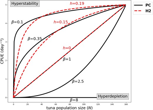
Illustration of hyperstability and hyperdepletion, as described by the power curve (PC; Equation 2) and Holling type 2 (H2; Equation 4) functions. Hyperstability occurs when CPUE reduces slower compared to the population size (0 < β < 1 for the power curve). Hyperdepletion occurs when CPUE reduces quicker compared to tuna population size (β > 1 for the power curve). H2 can describe hyperstability and no hyperdepletion since h ≥ 0. We used values of a and q such that CPUE=5 d−1 at N = 160.
Similar equations between a predator and its prey that describe consumption rate are traditionally referred to as trophic functions or functional responses in ecology, and provide the basis of mathematical models that are used in many studies of general predator-prey dynamics (Holling, 1959a; Arditi and Akçakaya, 1990; Tyutyunov and Titova, 2020). These trophic functions describe the average number of predations over time and per predator, given a predator and prey density, and have been used for species as diverse as predatory plants, birds, and carnivorous worms (Englund and Harms, 2001; DeAngelis et al., 2021).
Trophic functions are often defined as analytical functions, based on theoretical assumptions such as predator searching behaviour, but they can also be derived from individual-based model (IBM) simulations (Tyutyunov et al., 2008). In the context of tuna fisheries, a fisher can be thought of as a predator, tuna represent their prey, and a trophic function therefor gives the average tuna catch per fisher. As is shown for general predator-prey systems, heterogeneous distributions of predators and prey can result in trophic functional responses that have non-linear dependence on the prey and even the predator abundance (Arditi et al., 2001).
In the case of purse seine fisheries targeting tropical tuna, the heterogeneity of tuna distributions and their catch events is amplified by drifting Fish Aggregating Devices (dFADs) (Dagorn et al., 2001; Fonteneau et al., 2013). These free-drifting objects are deployed by fishers because they attract and aggregate pelagic species like tuna, concentrating both the biomass of target species and the fishing effort (Moreno et al., 2007; Leroy et al., 2013). This fishing mode developed in the 1990s, prior to which purse seiners targeting only ’free school’ tuna or those that were aggregated around naturally floating objects such as logs (Hampton and Bailey, 1993). The following two decades saw large-scale increases in the number of human-made dFADs being deployed (Maufroy et al., 2017), which now accounts for almost 50% of the catch in the WCPO, around 0.8–1 million tonnes annually (Williams and Ruaia, 2021). The drivers behind this attraction and aggregation of tuna to floating objects are not clear, but have been hypothesized to be driven by the social need to form large schools (Fréon and Dagorn, 2000; Capello et al., 2022), and that FADs may be indicative of productive areas for foraging (Leroy et al., 2013). In the presence of local depletion through fishing, such mechanisms may lead to both positive and negative feedbacks in the attractiveness of dFADs to tuna, and hence, such non-linear functional responses could in particular be present and provide a test case for the linearity assumption of the catch equation.
In this paper, we investigate the potential for non-linearity of tuna catch responses at the sub-grid scale (i.e. ≤ ∼ 1○) of ocean basin-scale tuna models. We investigate the catch response of dFAD-associated tuna, which provides a test case where a non-linear response is likely due to the heterogeneous distribution of both tuna and their catch events. We test how the catch response can be described analytically, by comparing catch responses in IBM simulations with analytical trophic functions under varying configurations of ocean flow, tuna behaviour, and fishing strategy, and across a range of tuna and dFAD density scenarios. We describe how these subgrid-scale factors influence the catch response, and the ability of linear and non-linear functional responses to appropriately describe the emergent catch rate at the 1○ grid-scale.
Methods
Catch per unit effort and local hyperstability
Catch Per Unit Effort (CPUE), also called catch rate, is often used as a proxy of the tuna population size, by assuming a linear functional response:
where C is the catch and E is fishing effort, q is the so-called catchability, which is a scalar representing the susceptibility of the fish stock to fishing. Although catchability is assumed to be a constant in this equation, in reality it may depend on the population size N (Rose and Kulka, 1999; Erisman et al., 2011; Ward et al., 2013; Hamilton et al., 2016). Alternative non-linear models have been proposed to describe the CPUE response (Harley et al., 2001; Maunder et al., 2006):
where coefficient q is independent of N, thus assuming that the true catchability is given by q′ = qNβ − 1. If β < 1, CPUE declines slower than tuna abundance, and the population is hyperstable. If β > 1, CPUE declines faster than the population size, which is referred to as hyperdepletion (Figure 1).
Here, we study the relationship between the catch rate and tuna density as a result of the fished aggregations that emerge from local-scale interactions between tuna, the prey that they forage upon, and dFADs. Focusing on ∼1○ scales, we use the terms hyperstability and hyperdepletion to describe the non-linear catch rate response at these local scales only. Non-linearity at these scales does not necessarily indicate the hyperstability or hyperdepletion of the tuna population, which typically occupies much larger areas. Identifying this would require applying such an IBM at larger spatiotemporal scales, considering the full population, which is not the aim of our study.
IBM and configurations
We use the individual-based tuna model (IBM) from Nooteboom et al. (2023), from which the general dynamics compare well with several types of observations (see Supporting Information Figure S1 for a summary of the processes in this IBM). In this model, both dFADs and tuna are modelled as particles, and the prey of tuna is a Eulerian field (from now on referred to as the forage field). Each tuna particle does not represent an individual tuna organism, but a school of tuna that interacts with both dFAD particles and the forage field (Becher et al., 2014; Meyer et al., 2017). While dFADs are only passively advected by ocean flow, tuna also swim towards dFADs if those are close enough (<10km), making a preference for dFADs with already associated tuna. Another driver of tuna movement is forage density. Tuna movement in the model is driven more towards areas of high prey abundance, with increasing stomach emptiness. Swimming towards areas with high prey abundance, they deplete the forage field and fill their stomach (see Nooteboom et al. 2023 for more details on stomach fullness modelling). We switched off the tuna-tuna interactions from Nooteboom et al. (2023), which generally did not have a substantial effect on the dynamics, to keep the number of required simulations in this paper computationally feasible. The model broadly replicates a number of observations from studies on tuna around drifting FADs, such as residence times of fish at FADs (Scutt Phillips et al., 2017), differences in relative stomach fullness between associated and unassociated tuna (Machful et al., 2021), and the aggregation of fish at FADs prior to targeting by purse seiners (Escalle et al., 2021b). A full description of these feedbacks and their emergent effects is given in Nooteboom et al. (2023).
Specific behavioural parameters in the model (κF and κP; Nooteboom et al., 2023) determine how strongly tuna are attracted towards dFADs and their prey. Overall, we distinguish between (i) dFAD dominant (κF = 1.5, κP = 0.5), (ii) forage dominant (κF = 0.5, κP = 1.5) and (iii) equal dFAD, forage (κF = κP = 1) behaviours, which determine the relative strength of swimming direction determined more by dFAD attraction, hunger-induced foraging, or both equally. These cases could apply to different tuna species or size classes, as smaller tuna species (e.g. skipjack tuna) generally show stronger dFAD associative behaviour compared to larger tuna species such as bigeye and yellowfin (Fonteneau et al., 2013).
We apply the IBM in idealized scenarios. Similarly to Nooteboom et al. (2023), we release N ∈ [5, 160] tuna particles and F ∈ [2, 40] dFAD particles at random locations in a rectangular domain |$[0,140\, \text{km}]\times [0,70\, \text{km}]$|, which is similar to a 1○ × 1○ scale. Note that we exclude lower numbers of tuna particles in Lagrangian simulations as it does not allow studying the catch rate functional response, and one dFAD particle does not allow random selection of dFADs by fisherman. Also, given the small domain size, it can be reasonably assumed that the habitat is suitable for the tuna in terms of abiotic environmental factors. We ran simulations for 100 days and skip the first 15 days before applying any further analysis of the catch rates (see Supporting Information Figure S2).
Three idealized ocean flow dynamics are modelled in separate settings, representing different oceanographic conditions. In the first, flow is assumed to be zero, and so all particles undertake a random walk, representing non-directional, diffusion-type movement (RWalk). The other two scenarios represent two idealized ocean flows, either Bickley Jet (BJet) (Bickley, 1937) or the Double Gyre (here denoted as the Double Eddy; DEddy) (Shadden et al., 2005). The BJet flow creates directional movement with ocean currents. The DEddy flow represents two meso-scale eddies, which accumulate passive particles in the middle through converging currents. These flow dynamics drive particle movement alongside the active, tuna behaviours described above. Similar to Nooteboom et al. (2023), we use zonally periodic boundary conditions for the particles in the BJet flow and reflective boundaries in all other cases, which is consistent with the flow in these configurations and assures that the particle densities (N and F) are conserved throughout the domain. See Nooteboom et al. (2023) for an overview of these configurations.
The interactive forage fields imply that once the forage density is initialized, it gets depleted by tuna and further redistributed, leading to dynamic and patchy fields. To be consistent with the flow, the redistribution of the forage field is simulated differently in each configuration. In case of BJet configuration, forage density is assumed to be lower in the North and South of the domain and higher in the middle of the jet; for the DEddy, it is higher in one of the two eddies compared to other parts of the domain; see Nooteboom et al. (2023).
A fishing event occurs every day at a single dFAD, where every dFAD-associated tuna particle is caught with a probability p = 0.5, which matches with observed biomass reduction near dFADs after a fishing event (Escalle et al., 2021b). Hence, fishing effort is kept constant across all simulations in this paper, which simplifies our consideration of CPUE. Tuna are released at a random location after their catch, assuming that other tuna enter the domain, so tuna density is kept constant during a simulation with a given number of particles.
Two different fishing strategies are tested in this paper, taken from Nooteboom et al. (2023). In the first fishing strategy (FSrandom), a fishing event occurs at a random dFAD, representing a situation in which fishers have only information on the location of dFADs and not the amount of associated biomass present. In the second fishing strategy (FSinfo), fishers are assumed to have information on the amount of tuna associated with a dFAD, and a fishing event is likely to occur at the dFAD that has most associated tuna particles (see fishing strategy FS3 in Nooteboom et al. (2023) for more details). Although FSinfo may appear more realistic compared to FSrandom, both are idealizations. FSrandom could be closer to reality in some cases. When there are many other floating objects, and dFADs are not equipped with echosounders, this information is hidden from the fisher, or the biomass estimate from the echosounder is unreliable (Baidai et al., 2020).
Simulations may be sensitive to the initialisation of the dFAD and tuna particles in the domain. Therefore, we apply 21 Monte Carlo simulations with different initial conditions, such that the average dynamics among the Monte Carlo simulations was insensitive to the addition of more simulations and allows investigating the spread among these simulations. Each simulation is initialized with different number of tuna particles from N = 5, ⋅⋅⋅, 160 in steps of 5, where each tuna particle represents a group of tuna individuals, and dFAD densities F = 2, 3, 4, 5, 7, ⋅⋅⋅, 40 in steps of 3. This corresponds to ~0.002 to 0.04 FADs per 10km2, which lies within typical range observed in equatorial waters fished by purse seiners in the WCPO (Escalle et al., 2021a). As the tuna particles do not represent individual tuna, but rather ‘super-individual’ minimal schools of tuna (Nooteboom et al., 2023), the calculation of tuna density represented in our simulations is less straightforward. Scutt Phillips et al. (2018) calculated the approximate minimal number of skipjack tuna of size prior to entry into the purse seine fishery, by converting weight and length of catch estimates from fishery observer records into numbers of fish, and using the smallest 5th percentile of school sizes indicated around 1000 fish. Taking this as an appropriate super-individual size, our examined tuna densities therefor lie between 5000 and 160 000 fish per square degree. These values are within typical densities predicted for floating object associated size-classes of both skipjack and bigeye tuna (Senina et al., 2018, 2020). For each combination of tuna and dFAD density, the particle movement is simulated in RWalk, BJet and DEddy configurations. The FSrandom fishing strategy is applied in the equal forage and dFAD tuna behaviour configuration, to reduce computational cost, while FSinfo fishing strategy was tested with all three movement behaviours. Hence, we ran 3 × 4 × 21 × 16 × 32 = 129, 024 simulations in total.
Trophic functions
In the framework of the classical predation theory (Lotka, 1925; Holling, 1959a; Arditi and Akçakaya, 1990; Tyutyunov and Titova, 2021), the fisher is a predator and tuna are prey. However, since fishers use dFADs as a tool to catch tuna, the interactions occur between tuna and dFADs, and the fishing event occurs at dFADs in our conceptual model. We may thus consider the dFAD as a proxy for the predator. The important difference between dFADs and the true predator is that not all tuna aggregations around dFADs lead to predation events, but the number of dFADs in the domain may impact the catch rates at “predatory” dFADs. Thus the relationship between time-averaged catch-per-unit-of-effort and tuna density in our simulations can be considered the functional response and modelled by the trophic function g, describing the average consumption of one predator per unit of time, or average catch per dFAD per day.
The simplest Lotka–Volterra trophic function (Lotka, 1925; Volterra, 1926) assumes a linear relationship of g and the prey density, modelling opportunistic predation and ignoring interactions between predators and prey:
where a > 0 is the predator searching efficiency and N the prey density. This LV trophic function is equivalent to a linear CPUE response (Equation 1) and likely not suitable as it does not allow us to account for a dFAD density effect or the effect of tuna-dFAD interactions.
Holling (1959a, b) assumed that predators need time h to consume a prey once it is found, and described a functional response by the equation
This is called the Holling type 2 functional response (H2). With both a, h > 0, H2 describes a linear increase of consumption at low prey density and a decrease in efficiency of predation for higher prey densities. In contrast to the LV function, H2 allows including the effects of predator-prey interference, existing in our modelled system via local depletion of tuna forage when tuna density becomes too high around a dFAD.
However, these two classical functions do not account for predator (i.e., the dFAD) interference. Beddington (1975) and DeAngelis et al. (1975) assumed that mutual predator interference reduces predation efficiency and proposed the following functional response (BDA) including the term with the predator density to H2:
where w > 0 measures the effect of the predator interference on the average consumption of predators.
Other forms of functional responses were proposed to describe specific predator-prey dynamics (Tyutyunov and Titova, 2020), as was shown by comparisons with empirical data for, e.g., mammals and sawflies (Holling, 1959a), microplankton (Harrison, 1995) or birds and fish in a wetland landscape (DeAngelis et al., 2021). However, no general functional response exists for all datasets, so to capture the specific dynamics emerging from the tuna-dFAD interactions in our model, we propose new functional forms adapted to our modelled system. By fitting these as well as the classical trophic functions Equations 3–5 to our IBM simulation data, we can establish the most suited functional forms describing the catch rates dependent on tuna-dFAD interactions within considered flow, movement and fishing strategy settings.
First, the catch rate functional response should include the positive effect of dFAD interference, i.e., account for observed phenomenon when the presence of other dFADs in the domain may stimulate the associative behaviour of tunas (Robert et al., 2013) and hence increase the catch rates. Such an effect, however, is expected only at low dFAD densities F. When dFAD densities increase further, they are more likely to ‘steal’ tuna from each other than when they are located closely together (i.e. their distance <10 km). Under information-poor fishing strategies, e.g. where random dFADs are targeted (FSrandom), this mechanism leads to a reduction of catch rates as the probability of targeting a dFAD with many associated tuna reduces. Under an efficient fishing strategy, where the dFADs with most associated tuna are targeted (FSinfo), this mechanism may still allow an increase of the catch rates with increased dFAD density, F, although this increase is expected to slowdown with F. Hence, we propose modifying the BDA function by including an additional term with the dFAD density:
This function has five parameters with m > 0, w1 > 0 and w2 > 0 and allows accounting for all above-described mechanisms: the opportunistic consumption, the tuna interference, and the dFAD interference increasing or decreasing catch rates. Let us consider particular cases of this function, including only one or several of these mechanisms. Selection of one of these simpler functions will allow emphasizing a particular mechanism that governs the tuna-dFAD interactions and consequently the catch rates.
First, if the catch rate response does not change with the density of tuna, then Equation 6 becomes simply
Aiming at capturing the hyperdepletion in the catch rate response, we also introduce to Equation 7 the power function type response with respect to the tuna density N:
with parameter β as in Equation 2 (Figure 1). Compared to Equation 2, this function accounts for the dFAD interference impacting the tuna catch rates. It can be simplified further for the specific case when w1 = 0, i.e., when increasing dFAD density can only improve the catch rates:
with constant w > 0, scaling the positive dFAD effect on tuna catch rates. Although such a functional response is expected only in case of selective (FSinfo) fishing strategy, this strategy is one of the most realistic corresponding to the modern dFADs equipped with echo-sounders and providing fishers with information about the dFAD associated potential catch. Another adaptation of the BDA function is to consider only positive dFAD impact on catch rates and the effect of tuna-dFAD interactions on the catch rates. Such a functional response is formalized by the following function:
Finally, the tuna-dFAD interactions may consist not only in a decrease of the fisher’s efficiency due to local forage depletion and consequent dFAD abandonment by tuna, but also when the tuna cannot associate with a dFAD due to other mechanisms, i.e., dominant flow dynamics, limiting tuna-dFAD encounter at small F. Such a functional response can be formalized using the term N/F instead of N in Equation 10:
Statistical analyses
We compared the output of the IBM simulations with the analytical trophic functions using the bootstrapping method of Tyutyunov et al. (2008). Since the IBM simulations vary among Monte Carlo simulations, the bootstrapping method can be used to obtain an uncertainty interval of parameter values when the trophic functions are fitted to the IBM simulation results. In this approach, we apply 2000 bootstrapping iterations where a random time-mean catch rate is drawn from the 21 Monte Carlo simulations, for every value of N = 5, ⋅⋅⋅, 160 and F = 2, 3, 4, 5, 7, ⋅⋅⋅, 40. The result is a two-dimensional matrix Y of size m = 17 × 32 = 544 with Y(F, N) the time-mean catch rate (number of individuals per fished day) for F and N. The trophic function is fitted to these data using nonlinear least squares.
In order to determine how well the fitted analytical trophic functions compare with the IBM simulation results, we used two measures for the goodness of fit. First, we used the normalized root-mean-squared error (NRMSE), which directly compares the average differences between the IBM simulation result and its fitted trophic function:
where Y,N, F is the catch rate from the IBM simulation for a given N and F value, |$\hat{g}$| is the trophic function fitted to matrix Y. We use the normalized version here, because it allows us to make comparisons between configurations. Second, we use Akaike’s information criterion (AIC) (Akaike, 1974), which does not only compare the direct difference between the IBM simulations and the trophic functions, but also penalizes the fit for the number of included parameters in trophic functions, and hence the complexity of the trophic function. We will compare the IBM simulation results to all trophic functions described in Table 1, to test which trophic function agrees most with the catch rate dynamics in the IBM in terms of NRMSE and AIC under different configurations.
Overview of the trophic functions that are compared to the catch rate responses from the IBM simulations in this paper.
| Name | Function | Reference |
|---|---|---|
| Lotka–Volterra (LV) | g(N) = aN | Lotka (1925); Volterra (1926) |
| Holling type 2 (H2) | |$g(N)=\frac{aN}{1+ahN}$| | Holling (1959a, b) |
| Beddington–DeAngelis (BDA) | |$g(N,F)=\frac{aN}{1+ahN+wF}$| | Beddington (1975); DeAngelis et al. (1975) |
| g1 | |$g(N,F)= \frac{aN}{1+ahN+w_1F+w_2F^{-m}}$| | This paper (Equation 6) |
| g2 | |$g(N,F)= \frac{aN}{1+w_1 F+w_2 F^{-m}}$| | This paper (Equation 7) |
| g3 | |$g(N,F)= \frac{aN^\beta }{1+w_1 F+w_2 F^{-m}}$| | This paper (Equation 8) |
| g4 | |$g(N,F)= \frac{aN^\beta }{1+w F^{-m}}$| | This paper (Equation 9) |
| g5 | |$g(N,F)= \frac{aN}{1+a h N +w F^{-m}}$| | This paper (Equation 10) |
| g6 | |$g(N,F)= \frac{aN}{1+a h \frac{N}{F} +w F^{-m}}$| | This paper (Equation 11) |
Results
Here, we examine the catch rate response from our simulations across values of tuna particle abundance N and number of dFADs F. We then describe the best fitting functional responses listed in Table 1, using AIC model selection criteria.
Figure 2 shows the median catch rate across N and F, and all tuna behavioural configurations, flow and fishing scenarios. As expected, catch rate increased with increasing tuna abundance N for all scenarios, but this was not always the case for increasing F. Fishing strategy had the greatest influence on catch rate, with FSinfo resulting in higher catch rates. At the same time, the tuna behaviour influences the non-linearity with respect to tuna abundance N. Thus, when tuna behaviour was forage-dominant under the RWalk scenario (no flow, only active movements to associate with dFADs or to forage), simulations showed the most non-linear response of catch rate with respect to N. This response can be explained by increased local depletion of the forage field around the dFAD, so tunas have to leave it to search for food, thus reducing catch rate.
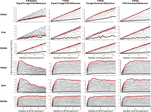
Median catch rate profiles, across ocean flow scenarios (rows) and fishing strategy-tuna behaviour configurations (columns). Median catch rate is plotted by number of dFAD particles F, across tuna particles N (top rows), and by number of tuna particles N, across number of dFADs F (bottom rows). The highest and lowest values of F (top) and N (bottom) are coloured in red and black, respectively.
Non-linearity in catch rate over F was present in all simulations, with catch rate increasing sharply from 2 to 7 dFADs. However, catch rate also fell with higher numbers of dFADs under some scenarios, most notably under the RWalk and BJet flow scenarios and FSrandom fishing strategy, i.e., when random dFADs were chosen for fishing.
To explore which scenarios led to hyperstability or hyperdepletion, we quantify the non-linearity in catch rate with tuna density N by estimating the β parameter from equation 2 for each value of F. Values of β > 1 indicate a hyperdepletion-like, and β < 1 a hyperstable-like response. Figure 3 shows the estimated values of β across dFAD density F, for the three ocean flow configurations, for three tuna behavioural scenarios, and for the fishing strategy used in the respective scenario.
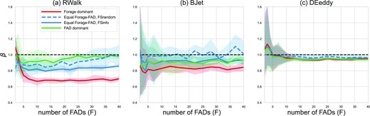
Non-linear catch rate response in the IBM simulations as expressed by the β value of the power curve for different tuna behaviours in the (a) RWalk, (b) BJet and (c) DEddy flow configurations. The power curve is fitted to the bootstrapped catch rates for every value of F. A value of β > 1 indicates a hyperdepletion-like response, a value of β < 1 indicates a hyperstable-like response. β = 1 indicates a linear catch response (horizontal dashed line). The shaded areas indicate the spread among bootstrapping iterations.
In general, non-linearity in catch rates with respect to tuna density N was weak under all scenarios. A hyperstable-like catch response was apparent only under forage dominant tuna behaviour, regardless of the ocean flow configuration of the simulations. First, in the IBM simulations with forage-driven individual behaviour, catch at dFADs is lower compared to scenarios with a stronger dFAD association behaviour of tunas (Nooteboom et al., 2023). Second, with increasing tuna density N, the local forage field depletion near dFADs negatively impacts the size of dFAD aggregations. Such a non-linear catch rate response was stronger under the RWalk configuration compared to other configurations (Figure 3). This is due to the prevalence of individual behaviour and consequent active movements in search for food over the passive transport by a flow.
Conversely, the DEddy flow configuration consistently exhibited the least non-linear catch rate, regardless of the tuna behaviour, fishing strategy, or dFAD density we examined. This is due to the converging eddy flows concentrating all dFADs, tuna particles, and fishing pressure into a very small area of the domain. At low dFAD densities, the stochastic nature of the Monte Carlo simulations results in increased variability in catch rate response, through the increased chance of many dFAD particles drifting into the centre of only one of the two eddies. This can focus fishing events in either the prey-rich or prey-poor eddies, depending on initial conditions, resulting in either a hyperstable or hyperdepletive catch rate for individual simulations.
Non-linearity in catch rate response was always weaker for fishing strategy FSrandom compared to FSinfo (Figure 3). Since an uninformed fisher does not necessarily find the largest aggregations, it interferes more rarely with the effects of tuna-FAD interactions, which lead to a non-linear response with respect to tuna density.
Finally, non-linearity also varied with dFAD density F, most notably under the RWalk flow configuration (Figure 3a). Under this configuration, the domain tends to have a more patchy forage field over time and a more hyperstable-like catch rate when compared to equivalent scenarios in the other ocean flow simulations. However, as F increases, fishing events more evenly sample the domain, reducing the degree of non-linearity in catch rate.
To establish the relationship between the time-averaged catch rate and density of tuna associating with dFADs, we fitted all analytical trophic functions listed in Table 1 to the simulated catch rates. We used AIC and NRMSE scores to select the trophic function that best describes the functional response emergent from tuna-FAD interactions within different flows and fishing strategies (Figure 4 and Supplementary Information Figure S3).
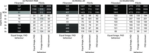
Average AIC between the median of the Monte Carlo IBM simulations and fitted analytical trophic functions (from Table 1), for every tested configuration (i.e. flow, fishing strategy and tuna behaviour). The lowest AIC is shown from 500 different initialisations before fitting. FSrandom refers to the fishing strategy where fishing events occur at a random dFAD and FSinfo where fishing events are likely to occur at the dFAD with most associated tuna. Lighter colors indicate lower AIC values. Notice that the AIC cannot be used to compare between columns, because AIC depends on the absolute catch values of the IBM simulations and hence such a comparison will not only represent a goodness of fit. See Supporting Information Figure S3 for the same figure but with the NRMSE. Dark boxes indicate a higher AIC and these colors are normalized for every column.
In general, the inclusion of dFAD density with both positive and negative, effects of dFAD interference on average catch rates greatly improves the fit to the simulated data compared to the classical trophic functions (LV, H, and BDA). In addition, under the FSInfo scenario, a positive effect of the dFADs interference on catch rates is predominant, as can be seen from AIC values for g4 and g5 functions (which account for a positive effect only) being close to those of g1 or g3. On the contrary, the negative effect of increasing dFAD density on tuna catch rates is more important for the uninformed fishing strategy FSRandom in the RWalk or BJet flow scenarios. Exclusion of the w1F term makes functions g4 to g6 unsuitable to describe the catch rate response to tuna-FAD interactions as LV or H functions, which do not include terms for dFAD density. The exception is the DEddy flow configuration, which results in qualitatively different relationships with N and F densities, whatever the fishing scenario (see Figure 2). Here, the negative effect of dFAD density is weak and positive effect of dFAD density is predominant in all cases, as functions g1 to g3 show similar scores to g4 and g5.
Let us now consider each flow separately and overview the functional responses depending on tuna movement behaviour and fishing strategy. In the RWalk flow scenario, catch rates from uninformed fishing with equal forage and dFAD behaviour and catch rates from informed fishing with dFAD dominant behaviour or tunas can be well described by functions g1 to g3. First, such similarity indicates that the contribution of tuna interference is minimal to these catch rates—the function g2 is linear with respect to N. Second, in both cases, increasing the number of dFADs negatively impacts the catch rates (Figure 2), meaning that dFADs may ‘steal’ tuna from each other, although the negative effect is less pronounced in an informed fishing strategy where fishers target the dFADs with the most associated tuna. In these two configurations, function g3 is only slightly better than others having best AIC and NRMSE scores.
Equal forage and dFAD behaviour of tunas with the RWalk flow and informed fishing result in catch rates that are well described by functions g3 and g4, with the latter being the particular case of the former function, and having the best scores. The forage-dominant behaviour in this configuration showed different relationships between catch rates and tuna and dFAD densities. Although functions g3 and g4 have good scores, the non-linear response to N is better described by a Holling type functional response, i.e. functions g1 and g5, among which g5 is selected due to its smaller number of parameters. The negative effect of dFAD interference is excluded from this functional response. As explained above, the non-linear response to N in the forage dominant behaviour, when there is no external flow, is attributed to faster local depletion of forage fields by increased densities of tunas, which are subsequently leaving dFADs in search for food.
In the BJet flow configuration, the uninformed fishing and equal forage and dFAD behaviour of tuna are best described by function g2 with the LV type response to tuna density and both effects of dFAD density, indicating a negligible contribution of tuna interference to the average catch rates. However, as g3 has the best fit to all other cases, and g2 is the particular case of g3, the latter can be selected as the most general trophic function describing the functional responses for all behaviours and fishing strategies in the BJet flow configuration. A minor non-linearity with respect to N is therefore best captured by the power function, with coefficient β ranging between 0.83 (forage-dominant behaviour) and 0.92 (equal forage and FAD behaviour).
Qualitative differences between the DEddy flow configuration and two other flow scenarios (Figure 2) indicate that the average catch rates in this configuration do not respond the same way to the dFAD density. Obviously, the flow dominates over tuna movements as behavioural response to external stimuli, as seen from very similar catch rate functional responses in all scenarios regardless of tuna behaviour or fishing strategy. Besides, at low dFAD density and high tuna density, the catch rates can be low, as tuna and dFADs can be advected to different eddies. The positive effect of dFADs on tuna aggregations and consequently catch rates is strong as well, but it is likely attributed to the flow and not to tuna behaviours. It is not surprising that function g6, allowing to account for reduced catch rates at low F and having only a positive effect of F density, fits the catch rates best in all scenarios. The best fit to the trophic function that was selected by the lowest AIC and NRMSE scores for each configuration, is shown in Figure 5.
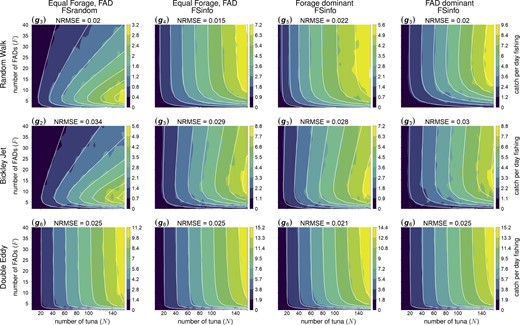
Median catch per day fishing (color scale) simulated by three conceptual models of the ocean flow (by row)–—zero flow (RWalk, top row), with Bickley Jet flow (BJet, middle row) and with Double Gyre flow (DEddy, bottom row), and three conceptual models of tuna movement behaviours combined with fishing strategy (by column)—equal forage and dFAD preferences with random selection of dFAD for fishing (FSRandom, first column), equal forage and dFAD with informed fishing (FSinfo, second column) and either forage dominant or dFAD dominant movement with informed fishing (FSinfo, third and fourth columns respectively). White isolines show the catch rate values computed by the trophic function (indicated for each panel) that fits best the simulated dataset. A lower NRMSE indicates a better fit between the simulations and the analytical function.
Discussion and outlook
In this study, we have presented IBM simulations of tuna and their interaction with drifting FADs across several idealized configurations of flow, forage fields, and fishing scenarios, at the 1○ and ∼100-day scale. We have modelled the changes in catch rate across varying tuna and dFAD densities and examined how this catch response depends on different model configurations. The IBM contains several interacting components that can induce feedbacks that impact the simulated catch and show that a hyperstable-like catch rate (i.e. a non-linear increase with respect to tuna density) can occur at the 1○ scale under certain configurations.
However, our results indicate that under the majority of the scenarios tested in this study, the degree of non-linearity in catch rate with respect to tuna density is very low. When present, it appears that it is the feedback mechanisms and heterogeneity between effort and spatial distribution of tuna in our model that cause the non-linear catch response that can be described as hyper stable. For example, in the RWalk scenario, we consider a system that is near-homogeneous in the absence of dFADs, with no flow, and with a homogeneous tuna-forage field. The introduction of dFADs into this domain leads to spatial heterogeneity and a non-linear catch rate response with respect to tuna density, which arise from tuna-FAD interference with a strength that depends on the behavioural configuration of both the tuna and fisher. This is due, under the assumptions of our simulation model, to the spatial concentration of tuna at the location of all fishing efforts, which is different from the otherwise homogeneous distribution of the population throughout the domain. In contrast, under the DEddy flow configuration, in which the flow concentrates both dFADs and tuna in the centre of eddies, we see a weaker non-linear catch response with respect to tuna density. While this scenario results in much higher catches, there is less disparity between the spatial concentration of fishing effort, and how the population is distributed throughout the domain. Compared to the RWalk scenario, the catch samples the true population more accurately in the DEddy flow.
More interestingly, however, we have also shown that the catch rate response of dFAD-associated tuna depends non-linearly on dFAD density. In all configurations, our simulations show that there exists a positive relationship between dFAD density and catch rates. Within a limited range of dFAD density, its increase leads to higher catch rates, whatever the fishing strategy. With further increase in dFAD density in the RWalk and BJet flows, the positive effect at low dFAD densities switches to negative in all scenarios of behaviours and fishing strategies, although in the RWalk simulations with informed fishing strategies, this effect is very weak through the modelled range of dFAD densities (Figure 2). These relationships demonstrate a quantitative link between the fishing effort in a region, which is fixed in all our scenarios, and the number of dFADs available to fishers in that region.
Our results imply the possibility that tuna catch rate response may become non-linear at the 1○ scale under some circumstances, in contrast to the linear catch rate response that is often used by basin-scale tuna models. Taking inspiration from classical trophic ecology, and testing the effectiveness of a suite of trophic functional responses, we have shown that the catch rate response of a single dFAD fisher is best represented by a non-linear function, with terms for both tuna and dFAD density. While different configurations can result in highly varied catch rate responses, our model selection exercise has revealed the four key dynamics emerging from the simulation, which are discussed below.
First, tuna interference may negatively affect catch rates, thus decreasing efficiency of fishers at higher tuna densities, and this effect is stronger when behaviour is forage-dominant. The mechanism behind this dynamics is local prey depletion near dFADs and consequent dFAD abandoning in search for food. Due to very weak observed non-linearity, such dynamics can be successfully described by a power function, although a Holling-type functional response is more suitable when the ‘predator–prey’ interactions are not influenced by a flow and the non-linearity is more pronounced. In our simulations, such a dynamic is realized in only in one configuration (RWalk with forage-dominant behaviour), demonstrating the degree that forage-dominant behaviour of tuna can alter the effectiveness of dFADs.
Second, at low dFAD densities (less than seven in our model domain), their increase always influences catch rate through a positive effect of increased attraction to dFADs, where fishing events then take place. Such an effect is also observed in natural systems and known as switching to associative behaviour when tuna swim to area with many dFADs (Robert et al., 2013). This requires an introduction of a dFAD density dependent term wF−m. Leading to an ‘optimal’ number of dFADs that maximizes catch rates, this dynamic appears in all configurations of the ocean flow scenarios, and shows fastest catch rate increase with number of dFADs in uninformed fishing strategy and highest catch rates in the flow-dominant DEddy simulations.
Third, when dFADs density is high enough that they get close to each other, their interference leads to the decrease in catch rates with increasing dFAD density. This dynamic is characterized by ‘fragmentation’ of aggregations with increased dFAD density, and it is well described by a BDA-type predator dependent term, with dFADs representing the proxy in our modelled system for a predator. As noted above, this dynamic was observed in configurations with RWalk and BJet flows, although this effect was very weak in RWalk simulations with the informed, FSInfo fishing strategy. Thus, trophic functions not accounting for this effect and there having one less parameter get an improved AIC score for equal and forage-dominant behaviours in this flow configuration.
Finally, the fourth dynamic is observed only in the flow dominant simulations (BEddy), where tuna and dFADs are transported by the flow to the centre of eddies, which results in decreased fisher’s efficiency at low dFAD densities. Such mechanism is described by a ratio-dependent term in function g6.
At present, linear relationships between catch and tuna abundance are assumed in the population dynamics models used to provide scientific advice in the WCPO (Hampton and Fournier, 2001; Senina et al., 2020). Although we find a notable, non-linear catch response with respect to tuna density at the 1○ scale only under certain circumstances in this paper, this does not necessarily imply the presence or not of hyperstability or hyperdepletion at the population scale. For example, it has been shown that even when local consumption of prey by predators (e.g. tuna caught by fishers) follows a linear function with respect to prey density, at larger spatial scales highly non-linear trophic relationship can emerge (Arditi et al., 2001). A non-linear catch response has been identified at the population level in many fisheries in which effort is spatially and temporally concentrated (Rose and Kulka, 1999; Hamilton et al., 2016; Feiner et al., 2020), and in some cases has been implicated in the collapse of a population of fish (Erisman et al., 2011). In particular for WCPO skipjack tuna, the stable, high catches of this species have caused speculation about potential hyperstability of the population (Vidal et al., 2020). Our idealized models presented here demonstrate that when fishing effort is concentrated at dFADs with the largest aggregations of tuna, particularly when other processes such as flow or forage field structure do not dominate tuna movement, such a non-linear catch response can emerge at the 1○ scale. This has clear parallels to the apparent increase in efficacy of purse seine vessels for finding tuna aggregations through echosounder buoys and other technology, although more complex than our idealized fishing strategies.
In our model, a catch event either occurs at a random dFAD (FSrandom) or more likely at the dFAD with most associated tuna (FSinfo). In reality, fishing strategies may be more sophisticated, with only some proportion of drifting dFADs in a particular region available to a particular fisher operating in that area. However, over the past decade, the instrumenting of dFADs with buoys that provide information on accumulated biomass has grown considerably, likely influencing the catch of fleets using them (Lopez et al., 2014; Maufroy et al., 2017; Kaplan et al., 2021). Fishing effort, and the resulting feedback on catch response that our model suggest, are also likely to change over time as communication of areas in which tuna density is high occurs between vessels. As more informed targeting of FAD-aggregated fish has increased, our results show the relationship between catch and abundance may have also changed over time, and in ways not normally captured by increases in catchability alone (Kaplan et al., 2021). Given the value of WCPO skipjack tuna as the largest tuna fishery in the world, with ∼2M tonnes landed annually (Williams and Ruaia, 2021), identifying and appropriately modelling the processes that may cause bias in estimations of tuna distributions and their abundance is necessary. Using information on dFAD density in the analysis of CPUE data for purse seine tuna fisheries has been discussed in several regional fisheries management organisations (Moniz and Herrera, 2019; Vidal et al., 2020). While the trophic functions we have explored in this paper may be too complex to be applied directly to the analysis of catch data, their response across different ocean flow and fishing strategy conditions should be considered in such work. For example, in areas where fishers have no, or less accurate, information on accumulated dFAD biomass, or where fishing occurs more opportunistically on floating objects, both positive and negative effects of dFAD density may influence catch rate. Future work should test the sensitivity of catch and tuna distributions to these trophic functions in ocean basin-scale models with more realistic fisheries. It may be that simply the addition of the dFAD density-dependent effect to the catch response is enough to obtain considerably different modelled tuna distributions, while the inclusion of hyperstability does not.
To test this, the IBM should be coupled to a more realistic hydrodynamic model and simulated at the ocean basin scale in order to investigate the relationship between catch and both tuna and dFAD density at the population scale. Here, we have considered idealized configurations that isolate the effects of diffusion (RWalk), strong directional flow (BJet), and strong particle accumulation (DEddy). Coupling of the IBM to a realistic hydrodynamic model also allows to test the functional response of tuna catch under more realistic flow scenarios.
Furthermore, although a major part of the total tuna catch consists of tuna that is associated with a drifting dFAD or other floating object (Leroy et al., 2013), it also consists of catch from free schools and anchored FADs. For instance, purse seine vessels may set gears on tuna near a dFAD at dawn, but also catch free-schooling fish opportunistically during the day. Using more types of fishing strategies may influence the catch response, and could be tested in future work. Moreover, assumptions other than the fishing strategy could be varied to test their influence on the catch response, such as differing boundary conditions and tuna-tuna interaction. While we have not explicitly explored this here, the social aspect of aggregation is implicit through the dFAD attraction movement vector, being function of the currently aggregating fish in our IBM. Nooteboom et al. (2023) also included tuna-tuna interaction terms operating throughout the model domain, which did have a small, typically negative, influence on simulated catch when included. Whether school fragmentation occurs, and has a subsequent impact on catch (Marsac et al., 2017), it is likely to be highly influenced by the interplay between the need to forage, social interaction, and depletion through fishing.
Finally, the IBM simulation we have used in this study remains a hypothesis-testing exercise, with many underlying assumptions that themselves should be tested where possible using real data or experiments (Kirby, 2001). The stark contrast present in the simulated catch response across ocean flow configurations could potentially be examined using ocean current observations alongside known dFAD density data. Analyses and standardisation of purse seine CPUE data should consider incorporating non-linear dFAD density covariates, particularly in regions where particles do not strongly accumulate. Similarly, further experiments to capture the dynamics of tuna around dFADs in the context of their biotic environment and local dFAD density may provide more information on the balance between behavioural motivations for aggregation at floating objects compared to that of foraging, to better inform models such as the one we have presented here (Dagorn et al., 2001; Perez et al., 2022).
Acknowledgement
Funding was provided by the Western and Central Pacific Fisheries Commission (WCPFC Project 42) and the European Union “Pacific-European-Union-Marine-Partnership” Programme (agreement FED/2018/397-941). This publication was produced with the financial support of the European Union and Sweden. Its contents are the sole responsibility of the authors and do not necessarily reflect the views of the European Union and Sweden.
Conflict of interest statement
The authors declare that they have no conflicts of interest.
Author contributions
Peter D. Nooteboom: Conceptualization, Methodology, Software, Validation, Formal analysis, Investigation, Data curation, Writing – original draft, Writing – review & editing, Visualization.
Joe Scutt Phillips: Conceptualization, Methodology, Writing – original draft, Writing – review & editing.
Inna Senina: Conceptualization, Methodology, Formal analysis, Writing – review & editing, Visualization.
Erik van Sebille: Conceptualization, Methodology, Software, Resources, Writing – review & editing, Project administration.
Simon Nicol: Conceptualization, Methodology, Writing – review & editing, Project administration, Funding acquisition.
Data availability
The code and data underlying this article are available in Zenodo, at https://zenodo.org/record/8024741.
