


Abstract
An assessment of the abundances and their trends is urgently needed for the conservation and management of fishery-targeted and rarely seen cetacean species (FTCS and RSCS, respectively); however, such assessment is often challenging because of the paucity of available data. In particular, the number of sightings is smaller than the general requirement for the reliable estimation of a detection function, and the spatial coverage of many cetacean surveys is insufficient. To address these issues, we propose a Bayesian approach that uses the previous abundance estimation of the same species or a species with similar biological traits as prior information. Therefore, we obtained the latest abundance estimates for six FTCS and two RSCS. For FTCS, we also estimated abundance trends by fitting an exponential population dynamics model with random effects accounting for interannual changes in animal distributions to the posterior samples of the Bayesian abundance estimates. Our approach enables us to (1) facilitate stakeholders’ consensus by maintaining previously agreed abundances while updating the conservation information; (2) identify the species of greater concern and prioritize conservation efforts towards those species; and (3) monitor the abundance and trends of data-limited cetacean species.
Introduction
The determination of the abundances of marine mammal populations and their trends is urgently needed, to provide fundamental knowledge indispensable for conservation and management, particularly for fishery-targeted cetacean species (FTCS) and rarely seen cetacean species (RSCS; e.g. threatened species and species with low abundance). However, robust estimations of the abundance of marine mammals are often challenging. Many marine mammal species are not frequently encountered, and sufficient funding and human resources are required to survey their wide, and sometimes oceanwide, distributions. Such a data-limited situation is often encountered during the assessment of fisheries and wildlife populations (Chrysafi and Kuparinen, 2015; Dowling et al., 2019; Punt et al., 2021). The abundance of cetaceans inhabiting open oceans is primarily estimated using the line-transect sampling technique (Hammond et al., 2021). The core part of the line-transect analysis consists of the estimation of the detection, which is probability dependent on the perpendicular distance between the observer and the detected schools using a so-called detection function (Buckland et al., 2001). At least 60–80 sightings are required to estimate detection function reliably (Buckland et al., 2001); however, this requirement was not met in many field samplings of cetaceans because of the infrequency of their encounters (e.g. Kanaji et al., 2018).
Delphinidae is the most diverse living family among cetaceans and comprise 37 species according to the latest version of the Society for Marine Mammalogy List of Marine Mammal Species and Subspecies (Committee on Taxonomy, 2022). Among them, most oceanic delphinids are listed as being “Least Concern” on the latest version of the IUCN Red List, although some species assessments included the caution that the current listing should be considered provisional (pending) based on difficulties in detecting the population trend because of insufficient data (e.g. Braulik, 2018; Kiszka and Braulik, 2018a). Even for species listed as having “considerable abundance”, a lack of sufficient time-series of abundance estimates needs to be resolved (Kiszka and Braulik, 2018b). The low frequency of surveys at an adequate ecological scale restricts the depth of time-series; and consequently, the statistical power to precisely evaluate the trends. Particularly in the coastal waters off Japan, several delphinid species are currently targeted by dolphin fisheries and thus a current population status needs to be carefully monitored (Kasuya, 2017). Nevertheless, recent trends in their abundances have not sufficiently evaluated for these FTCS.
Line-transect surveys aimed at estimating the abundance of small cetaceans, mainly delphinid species, were first established in 2006–2007, with the second phase taking place in 2014–2015 in the waters covering Japan’s exclusive economic zone off the Pacific coast and around the southwestern islands in the form of a small cetacean survey programme (Figure 1), the Japan Fisheries Research and Education Agency Cetacean Sighting Survey (JAFRACSS; Kanaji et al., 2018, 2021). Based on these surveys, the time-series of abundance estimates for FTCS, i.e. the common bottlenose dolphin (Tursiops truncatus), Risso’s dolphin (Grampus griseus), the southern form of short-finned pilot whale (Globicephala macrorhynchus), the rough-toothed dolphin (Steno bredanensis), the pantropical spotted dolphin (Stenella attenuata), and the melon-headed whale (Peponocephala electra), were published by Kanaji et al. (2018). Dolphins are often encountered in large schools; thus, the total number of encountered schools tends to be much smaller than the total counts of individual animals. For almost all species, the number of schools encountered during these surveys was <60 in each single year, which was insufficient for the robust estimation of the detection function. In Kanaji et al. (2018), to estimate the detection function, the survey data from these two phases were pooled, followed by additional combination with data from the other surveys in 1985 and 1992 that did not specifically target delphinid species. Year-related effects were included as additional covariates into the detection function (e.g. Kanaji et al., 2018). Such treatment of sharing the information across the different survey years was an effective compromise to estimate the abundance of species that are less frequently encountered, such as delphinids off the coast of Japan. However, the combination and pooling of new data obtained from the recent surveys with past data would cause another difficulty, because updating the detection function simultaneously implies updating the past abundance estimates. Combining the data and updating the model would be useful for reducing uncertainty in abundance estimations and modifying the management direction in terms of adaptive management (Hilborn and Walters, 1992). However, the current management decision was established based on the past assessment of abundance. Updating the recent abundances and modifying the management and conservation directions while retaining previous analytical results might be an option towards constructive argumentation among stakeholders with different interests. This practical approach is expected to promote the establishment of a consensus among stakeholders more easily, because they could keep previously agreed abundances while engaging in debate based on newly obtained information.
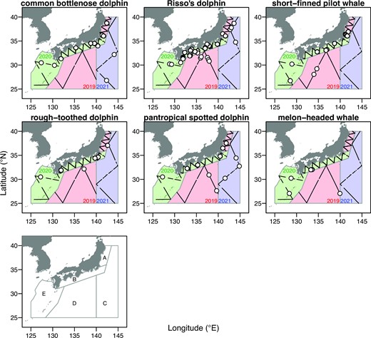
Track lines of the latest surveys (Fisheries Research and Education Agency Cetacean Sighting Survey, FRACSS) conducted in 2019–2021 and sighting positions of six FTCS. The survey area was stratified into five blocks, A (18890.89 square nautical miles, nmi2), B (44095.38 nmi2), C (182656.36 nmi2), D (213731.42 nmi2), and E (120949.01 nmi2).
Recently, Bayesian modelling has been widely used in line-transect analyses because it offers numerous benefits for assessing animal abundance (Eguchi and Gerrodette, 2009; Gerrodette and Eguchi, 2011). Differentiating the formulae is often difficult for complicated hierarchical model in the context of conventional maximum likelihood approaches. Bayesian frameworks can more explicitly deal with the hierarchical structures in line-transect analyses and permit the simultaneous estimation of all parameters from several modelling components through variance propagation (Eguchi and Gerrodette, 2009; Pardo et al., 2015; Kanaji and Gerrodette, 2020). Probabilistic inference derived from Bayesian methods permits direct use of the results in decision making (Punt and Hilborn, 1997). In terms of the assessment of data-limited populations, the Bayesian approach offers the benefit of being able to incorporate prior information based on historical datasets or expert knowledge (Punt and Hilborn, 1997). Even when a sufficient number of samples are not obtained from a single-year survey, such as that observed for FTCS, we can construct models using prior information from the parameters of a previous abundance estimation, and the uncertainty caused by the small sample size could be taken into posterior distributions. This approach would also be beneficial for the assessment of the abundance of RSCS. If neither previous information nor expert knowledge exist, it would be practical to borrow prior information from a closely related species or a species with similar appearance and behaviour. Borrowing important parameters from extensively studied species with a similar life history has been relatively commonly used for stock assessment in the setting of data-limited fisheries (Punt et al., 2011; Chrysafi and Kuparinen, 2015).
Information of temporal trends in the population abundance is important particularly for conserving and managing of FTCS, because it is needed to assess how human-cause mortality affects entire population status (Wade, 1998; Punt et al., 2020). For the situation in small sample size and relatively large uncertainty in time-series abundance estimates, fitting a simple population dynamics model to the time-series of population abundances with prior information might be an effective solution to estimate recent trends (Authier et al., 2020; Kanaji et al., 2021). However, in many cases, entire population abundance itself cannot be obtained for each single year because of wide distribution ranges of many cetacean species (Skaug et al., 2004; Hakamada et al., 2017). For example, in the past surveys of JAFRACCS, three vessels simultaneously covered different survey blocks. Despite such efforts, it was difficult to survey many blocks in the management area sufficiently in a single year. In the latest programme deployed in 2019–2021, only one vessel was involved, and 3 years were required to completely survey the entire area. In the dynamic ocean environment, cetacean habitat could shift year to year, which potentially cause uncertainty in total (combined) abundance estimates (see Appendix 1). International authorities on marine mammal conservation and management (e.g. International Whaling Commission and North Atlantic Marine Mammal Commission) has recommended to assess such additional variance to the abundance estimates from multi-year surveys (Øien, 2009; Matsuoka et al., 2011; Solvang et al., 2015; Leonard and Øien, 2020). A standard procedure for this purpose has been established by Skaug et al. (2004), in which a simple exponential-growth population dynamics model is fitted to the nominal abundances from different blocks/years with random effects accounting for distribution changes.
The objectives of this study are twofold. The first objective was to estimate the latest abundances of both FTCS and RSCS using Bayesian line-transect analyses with prior information from the previous abundance estimation of the same species or species with similar biological traits. The third-phase small cetacean survey, which was a part of the JAFRACSS programme, was completed in 2019–2021 and covered survey areas that were almost the same as those assessed in the first and second phases (Figure 1). The abundances of the following eight species were estimated using this approach: common bottlenose dolphins, Risso’s dolphins, short-finned pilot whales, rough-toothed dolphins, pantropical spotted dolphins, melon-headed whales, Fraser’s dolphins (Lagenodelphis hosei), and pygmy killer whales (Feresa attenuata). For short-finned pilot whales, only southern forms were targeted for the study. The main habitat of the northern forms is outside of the study area and the northern forms are easily and visually identified by their white saddle patch (Kanaji et al., 2011). The former six species are FTCS mentioned above, whereas the latter two species are RSCS for which abundance had not been assessed previously. The second objective was to estimate abundance trends by using abundance estimates with spatially partial coverages. Here, we developed a simple population dynamics model with random effects for distribution changes using posterior samples of Bayesian abundance estimates as input data as in Skaug et al. (2004). This approach enables us to appropriately deal with large uncertainties caused by spatiotemporal variation by utilizing all abundance information from different years/blocks. Only FTCS was targeted for this analysis, because assessing the effect of direct catch is particularly required for these species. Even if trend is estimable, its validity cannot be assessed because of a lack of supplementary information such as catch statistics and distribution patterns for RSCS. For these estimated abundances and trends, we discussed the future directions of the conservation and management of delphinid species, both FTCS and RSCS, in the waters off the Pacific coast of Japan.
Material and methods
Field data (FTCS)
Sighting surveys dedicated to delphinid species were conducted in the areas off the Pacific coast of Japan and around the southwestern islands (Figure 1). The entire area was divided into five blocks (A–E). These blocks were originally designed to cover the main habitat of bottlenose dolphins (Kanaji et al., 2022) and southern short-finned pilot whales (Kanaji et al., 2015), and the total abundance across these blocks has been used for the management and assessment of the six delphinid species (Kanaji et al., 2018). Survey cruises were carried out three times in different years. RV Kaiyo-maru No. 7 (649 GT, Kaiyo Engineering Co., Ltd) was used in all 3 years, albeit using different equipment from that employed in some of the past surveys, as discussed below. These cruises covered blocks A and D from 21 May to 8 July 2019; blocks B and E from 19 May to 6 July 2020; and block C from 1 to 28 June 2021, respectively (Figure 1). The same block design has been used in small cetacean surveys since 2006 (Appendix 2; Supplementary Figure S1). The configuration of transect lines was designed using the “equal spaced zig-zag” option in the Distance software, version 7.3 (Thomas et al., 2010).
The vessel ran on the transect lines at ∼11.5 knots (≈21.3 km h−1), to mitigate the impact on the animal’s swimming behaviour (Buckland et al., 2001), and two experienced observers searched for marine mammals within an area covering from left abeam (−90° from the track line) to right abeam (90°) using binoculars (7 × 50) from the top of a barrel placed at 18 m above the water line. The search was continued whenever weather conditions permitted (Beaufort scales = 4.0 or lower) during the daytime in the survey periods. When cetacean schools were encountered, the observers estimated the radial distance and the angle from the vessel to the detected schools using scaled binoculars and an angle board. A closing mode was adopted for JAFRACSS small cetacean surveys; therefore, the vessel approached the detected cetacean schools to identify species and estimate school size.
Field data (RSCS)
In addition to the dataset from the latest surveys mentioned above, we used the past survey data collected from 2006 to 2015 (Figure 2). The abundances of Fraser’s dolphins and pygmy killer whales have not been estimated to date because their sample sizes in each single year were too small. Therefore, we pooled the data from the past and latest surveys to estimate the detection function and mean school size. Fraser’s dolphins were encountered in blocks C and D (only in the northern subblock) in 2007; blocks C, D, and E in 2014; and blocks B, C, and D in 2019–2021. In contrast, pygmy killer whales were encountered in block D (only in the southern subblock) in 2007; and in block E in 2014, 2015, and 2020 (Figure 2). The survey protocol used in the past surveys was identical to the latest one. Details of the standard data collection methods used in the JAFRACSS small cetacean surveys are provided in Kanaji et al. (2018).
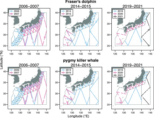
Track lines of the past (2006, 2007, 2014, and 2015) and latest FRACSS programmes (2019–2021) and sighting positions of two RSCS. Some survey blocks were further divided into two or more subblocks in the past surveys.
Basic line-transect formulae
We adopted a standard line-transect approach for estimating abundance (Buckland et al., 2001). The following two types of detection functions were considered to fit to perpendicular distances:
where xi is the perpendicular distance of the i-th sighting calculated by simple trigonometry from the recorded angle and radial distance. A scale parameter |${\sigma }_i$| is estimated for the half-normal model, while shape parameter |$\theta $| as well as |${\sigma }_i$| are estimated for the hazard-rate model. Here, we considered multi-covariates into the detection function, so that |${\sigma }_i$| is expressed as a linear combination of covariates that potentially affect the detection probability, such as weather conditions and school size (Marques and Buckland, 2003),
where zi is a vector of multi-covariates (the first component is always one) and |${\boldsymbol{\alpha }}$| is a vector of coefficients that indicate the effect of corresponding covariates.
The integration of the detection function g(x) over x represents the effective strip half-width (w) within which all animals are perfectly detected if all assumptions are met (Buckland, ). Thus, the total abundances in the j-th block (|${\hat{N}}_j$|) and year y can be obtained as follows,
where Aj and Lj,y are the area and total length surveyed in block j and year y. The probability of detection on a track line, g(0), was assumed to be 1.0 for all species, as assumed in our previous analyses (Kanaji et al., 2018). The observed school sizes are likely larger in larger perpendicular distances; thus, the corrected mean school size (|${\hat{s}}_j$|) was estimated via regression of the school size on the detection function g(x).
School sizes (|${s}_i$|) minus 1 are assumed to follow a negative binomial distribution with the mean |${\lambda }_i$| and the dispersion parameter |${\phi }_\lambda $|. The dispersion parameter |${\phi }_\lambda $| allows for highly variable dolphin school sizes generally ranging from one to several hundred individuals (Kanaji and Gerrodette, 2020). The encounter rate (|${n}_{j,y,k}/{L}_{j,y,k}$|) was modelled as follows,
where the expected encounter rate in specific block j in year y was parameterized as random intercept |${b}_{j,y}.\ $|This random effect enables us to naturally estimate abundance in the blocks without any sightings, because no sightings are not necessarily equivalent to zero animals inhabiting the block. Here, the sampling unit was a track line deployed in each block, so that |${n}_{j,y,k}$| and |${L}_{j,y,k}$| represent the number of encountered schools and track line length, respectively, at the k-th track line in block j. Parameters for all these models were estimated within a Bayesian framework. The Bayesian posterior probabilities for all parameters were sampled from Hamiltonian Monte Carlo (HMC), which is a family of Markov chain Monte Carlo (MCMC) algorithms, using Stan version 2.19.2 (Stan Development Team, 2020) and the R interface “Rstan”. The numerical integration of the detection function from x = 0 to 3 miles was made based on the 15-points Gauss–Legendre quadrature (Golub and Welsch, 1969; Smyth, 1998). The nodes and weights were generated using the R function “gauss.quad” in the package “statmod” (Smyth et al., 2022). We ran the model with three chains, each consisting of 30000 iterations with a burn-in of 10000 and retained every tenth value. All these analyses were done separately by species.
Prior information (FTCS)
To estimate the model parameters in the multi-covariate detection functions for FTCS, we used previously estimated parameters and the covariance matrices as informative prior distribution (Table 1). Here, we assumed a multivariate normal distribution for the prior detection parameters. According to the previous analyses, a half-normal model was used for rough-toothed dolphins and a hazard-rate model was used for the remaining five FTCS (i.e. common bottlenose dolphins, Risso’s dolphins, short-finned pilot whales, pantropical spotted dolphins, and melon-headed whales; Kanaji et al., 2018). The Beaufort scale was taken as a covariate that significantly affected the detection probability for Risso’s and spotted dolphins, whereas vessel type was adopted for rough-toothed dolphins (Kanaji et al., 2018). Vessel type is among the important covariates that potentially affect detection probability. Although several vessels were used in the past and latest surveys of the JAFRACCS programme, they were typically categorized into two vessel types (former whaling vessel or multi-use research vessel), both of which were equipped with a top barrel; however, whaling-type vessels were previously involved in commercial whaling, and thus their crews were considered more experienced for cetacean surveys. The research-type vessel RV Kaiyo-maru No. 7 was used in the surveys performed in 2019–2021. The vessel’s equipment was generally similar to that of the research-type vessels used in the previous surveys (e.g. the height of the observation platform, speed while approaching the encountered schools and crews experience). No covariates were considered for estimating the detection functions of common bottlenose dolphins, short-finned pilot whales, and melon-headed whales based on the previous knowledge. On the other hand, Beaufort scale is often an important covariate, which affects a detection probability (Buckland et al., 2001), so that we additionally incorporated the Beaufort scale for these three species, and compared the models with/without a covariate based on widely applicable information criterion (WAIC; Watanabe, 2013). We also tested the model with the Beaufort scale covariate for rough-toothed dolphins. For school size regression, the previous estimates and covariance matrices by Kanaji et al. (2018) were also used as multivariate normal prior data for parameter combination of |${a}_1$| and |${a}_2$| for the six FTCS mentioned above. This approach was reasonable because the ranges of the data collected in 2019–2021 were generally within those used in Kanaji et al. (2018) (Appendix 2; Supplementary Figure S2). The data from the surveys not specifically targeted small cetaceans were additionally combined to estimated detection functions in the previous analyses, so that priors used here included information from the surveys since 1985. However, the designs of track lines and blocks before 2006 were quite different from recent JAFRACCS small cetacean survey. We have not used data before 2006 for further analyses. Non-informative uniform priors were used for the parameter |${\beta }_b$| and uniform priors with wide intervals (0−100) were used for |${\sigma }_b$| in the encounter rate model.
The past abundances for six delphinid species estimated by Kanaji et al. (2018).
| Species | Year | A | B | C | D | E |
|---|---|---|---|---|---|---|
| Common bottlenose dolphin | 2006 | 8 021 (0.85) | 2 673 (0.97) | - (-) | 0 (-) | 34 811 (0.57) |
| 2007 | 0 (-) | 4 283 (0.76) | 14 198 (1.14) | 6 122 (0.98) | - (-) | |
| 2014 | 0 (-) | 3 535 (0.98) | 0 (-) | 0 (-) | 40 994 (0.59) | |
| 2015 | - (-) | - (-) | - (-) | - (-) | 15 982 (0.70) | |
| Risso’s dolphin | 2006 | 1 091 (0.76) | 15 812 (0.39) | - (-) | 5 001 (0.75) | 17 894 (0.41) |
| 2007 | 6 961 (0.57) | 16 272 (0.41) | 13 612 (0.79) | 3 876 (1.03) | - (-) | |
| 2014 | 5 805 (0.57) | 28 956 (0.35) | 35 417 (2.00) | 12 939 (0.47) | 61 046 (1.02) | |
| 2015 | - (-) | - (-) | - (-) | - (-) | 6 133 (0.83) | |
| Short-finned pilot whale | 2006 | 808 (1.19) | 0 (-) | - (-) | 11115 (0.55) | 17 483 (0.48) |
| 2007 | 0 (-) | 1 899 (0.57) | 11 688 (0.89) | 0 (-) | - (-) | |
| 2014 | 0 (-) | 1 533 (0.79) | 6 877 (1.29) | 11 305 (0.55) | 11 853 (1.34) | |
| 2015 | - (-) | - (-) | - (-) | - (-) | 4 032 (0.83) | |
| Rough-toothed dolphin | 2006 | 0 (-) | 299 (0.95) | - (-) | 4 309 (0.60) | 0 (-) |
| 2007 | 0 (-) | 0 (-) | 5 606 (0.68) | 451 (1.05) | - (-) | |
| 2014 | 0 (-) | 1 769 (0.85) | 0 (-) | 3 260 (1.76) | 0 (-) | |
| 2015 | - (-) | - (-) | - (-) | - (-) | 9 531 (0.82) | |
| Pantropical spotted dolphin | 2006 | 0 (-) | 3 678 (0.67) | - (-) | 92 781 (0.56) | 11 676 (0.55) |
| 2007 | 0 (-) | 3 596 (0.90) | 36 322 (0.56) | 27 481 (0.44) | - (-) | |
| 2014 | 0 (-) | 11 086 (0.51) | 58 003 (0.52) | 54 488 (0.55) | 7 141 (0.79) | |
| 2015 | - (-) | - (-) | - (-) | - (-) | 18 967 (0.85) | |
| Melon-headed whale | 2006 | 0 (-) | 0 (-) | - (-) | 18 557 (0.63) | 17 525 (0.52) |
| 2007 | 0 (-) | 5 436 (0.70) | 20 075 (0.60) | 17 901 (0.57) | - (-) | |
| 2014 | 0 (-) | 2 627 (0.85) | 29 452 (0.68) | 19 367 (0.56) | 5 076 (0.94) | |
| 2015 | - (-) | - (-) | - (-) | - (-) | 0 (-) |
Prior information (RSCS)
We had no prior information on the parameters of abundance estimation models for two RSCS, Fraser’s dolphins and pygmy killer whales; thus, we borrowed prior distributions from FTCS to construct line-transect models of these RSCS. We first chose three candidate models (models M1–M3) based on the similarity criteria in the ecological traits of the six FTCS to each RSCS: body shape (appearance), body size, and school size, and then compared these models based on WAICs. The appearance of Fraser’s dolphins, with a grey-coloured body and a short beak, resembles closely those of common bottlenose dolphins (M1). Their mean body mass [95.4 kg (females) and 95.4 kg (males)] was closer to that of melon-headed whales (M2) [105 kg (females) and 104 kg (males); Trites and Pauly, 1998]. The mean value of the observed school size was closer to that of pantropical spotted dolphins (M3; see the Results section). Therefore, we used multivariate normal priors of these three FTCS for Fraser’s dolphins for the parameters of both detection functions (equations 1 and 2). Pygmy killer whales have a medium-sized body and a rounded head, and their appearance closely resembles that of melon-headed whales (M1). Their mean body mass [78.0 kg (females) and 117 kg (males)] was closer to that of rough-toothed dolphins (M2) [87.7 kg (females) and 96.3 kg (males); Trites and Pauly, 1998]. The mean and range of the observed school size were closer to those of Risso’s dolphins (M3; see the Results section). Multivariate normal priors of these three FTCS were used for pygmy killer whales. All covariates included in the original models were considered for RSCS, whereas the covariate of vessel was not used for pygmy killer whales. No pygmy killer whale sightings were reported from the whaling-type vessels during the past surveys. For the estimation of mean school size, non-informative priors were used without linear regression, because neither of the two species showed a clear tendency for an association between school size and perpendicular distance (Appendix 2; Supplementary Figure S2). Similar to FTCS, uniform priors were used for the parameter |${\beta }_b$| and |${\sigma }_b$| in the encounter rate model.
Trend analysis and PBR
To evaluate additional variances for multi-year surveys, we assumed an exponential population growth to evaluate additional variances according to Skaug et al. (2004). A simple idea to fit a population dynamics model to partial abundance estimates from multi-year surveys is to combine abundance estimates from different years/blocks and treat it as if from entire population size in a single year. However, our simulation tests (Appendix 1) show that such approach could not estimate abundance trend precisely because the assumption that the abundance combined from different years represents the total abundance in a single year is incorrect. Additional random effect term is needed to account for year-to-year changes in animal distributions. Background ideas and simulation tests for the random effects model are summarized in Appendix 1.
Let the total abundance within the blocks A–E in 2014 be |$N_{2014}^{tot}$|; then, the total abundance in year y is given by:
where R is the rate of growth (or decline) in population abundance. Total abundance covering entire study areas were not obtained except for 2014, because we spent 2–3 years to complete surveying all five blocks and have abundance estimates only from 1 to 4 blocks in 2006, 2007, 2015, 2019, 2020, and 2021, respectively (Appendix 2; Supplementary Figure S1). Here, the total abundance |${N}^{tot}$| was parameterized to the year 2014 when all five blocks were completely surveyed in a single year. The theoretical maximum population growth rate is often considered to be 4% (Wade, 1998), and those estimates were reported ∼3–4% from the field surveys for delphinid species (Kasuya, 1976; Olesiuk et al., 1990; Mannocci et al., 2012). Currently, the annual catch limit for FTCS is up to 1% of the latest abundance (Kanaji et al., 2021), whereas other sources of mortality (e.g. environmental changes, competition, diseases, ship strike, etc.) might also cause decreases in abundance. Here, we assumed 0.95 and 1.04 as the lower and upper bounds for R, respectively (i.e. −0.051 and 0.039 for min and max log R). Any prior information other than upper and lower limits was not given for R.
We randomly sampled 5000 sets of abundances using means and CVs of previous estimates by Kanaji et al. (2018). The 5000 sets of abundances were also randomly sampled from posterior distributions of those for 2019–2021, and the sum of sampled abundances in the blocks A–E was used as the total abundance in 2020. Individual draws from the posterior distribution of abundance estimates (|$\hat{N}_y^{samp}$|) were fitted to the above exponential model using the following Poisson distribution. Year-to-year changes into their spatial distribution are introduced using the random effects parameter |${\xi }_{y,j}$|.
where the fixed-effects parameter |${\delta }_j$| accounts for the relative importance among the blocks in the reference year, and the random-effects parameter |${\xi }_{y,j}$| accounts for the overdispersion caused by interannual changes in dolphin distributions from that year (Skaug et al., 2004). We set the reference year to 2014; thus, |${\xi }_{2014,j}$| was assumed to be zero for all block j, because we had the most sufficient information on abundances and their variations among the blocks in that year. For the other years in which some blocks had not been surveyed, we assumed that |${\xi }_{y,j}$| follows a normal distribution with a mean of 0 and a variance parameter |${\sigma }^2$|, the so-called the additional variance (Skaug et al., 2004). Sampled abundances in block j and year y were assumed to follow a Poisson distribution.
The reason why we used Poisson was that several species had zero abundance estimates in specific blocks and years in the previous estimates (Kanaji et al., 2018), and a Poisson distribution naturally models zero observations. Unexplained overdispersion by Poisson distribution was expressed by a random effect with additional variance |${\sigma }^2$|. To fit the Poisson model to |$\hat{N}_{y,j}^{samp}$|, the values obtained from the line-transect analysis were simply rounded off to the nearest integer. These analyses were considered for FTCS exclusively. Because the abundance estimates of RSCS are zero in many blocks and years, there will remain substantial variations that cannot be estimated from the mixed-effect models. We used a Laplace approximation for estimating trend models using the template model builder (TMB, Kristensen et al., 2016), because a much faster computation approach is desirable for repetitive evaluations.
We calculated potential biological removal (PBR) using the total abundances by simply combining from different blocks/years and those by above additional variance models. PBR is defined as:
where |${N}_{MIN}$| is the 20th percentile of abundance estimates, |${R}_{MAX}$| is the intrinsic growth rate, and |${F}_R$| is the recovery factor (Wade, 1998). The default parameters provided by Wade (1998), |${R}_{MAX} = 0.04$| and |${F}_R = 0.5$|, were used to calculate PBR.
Results
Block-specific abundances (FTCS)
During the survey period of 2019–2021, a total of 31 track lines of 3913.71 nautical miles (nmi) were surveyed; 415.42 nmi in block A, 973.28 in B, 861.82 in C, 982.06 in D, and 681.13 in E. Within these areas, a total of 13, 37, 18, 6, 11, and 5 school sightings were recorded for common bottlenose dolphins, Risso’s dolphins, short-finned pilot whales, rough-toothed dolphins, pantropical spotted dolphins, and melon-headed whales, respectively (Table 2). Theoretically, the detection probability is expected to be higher when a school is sighted close to the track line, whereas it decreases with increasing perpendicular distance. However, the current dataset did not show this typical tendency because of the insufficient number of sighting records for a few species (e.g. pantropical spotted dolphins and melon-headed whales, Figure 3). Thus, we used species-specific detection functions previously obtained as prior information. After 30000 iterations, the models sufficiently converged with the Gelman–Rubin statistic |$\hat{R}$| smaller than 1.1 for all estimated parameters (Gelman et al., 2014). For common bottlenose dolphins, short-finned pilot whales, and melon-headed whales, the models with/without the Beaufort scale covariate were compared based on WAIC. By adding the covariate, WAIC was improved from 188.2 to 187.7 for common bottlenose dolphins. For short-finned pilot whales and melon-headed whales, on the other hand, WAICs for the models without the Beaufort scale covariates were 251.3 and 99.4, respectively, still smaller than 253.2 and 103.7 for the models with the covariates. The model with the vessel-type covariate was 83.1 for rough-toothed dolphins, while 85.9 for the model with Beaufort scale covariate.
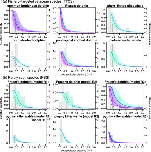
Histograms of perpendicular distances obtained in the latest JAFRACSS survey (2019–2021). Open histogram is for Beaufort scale > 3, and filled histogram is for ≤ 3 when multi-covariate detection functions were applied. Solid lines and colour filled areas represent median and 95% credible intervals of posterior distributions (red for Beaufort scale > 3 and blue for ≤ 3 for multi-covariate detection functions). Dotted lines represent the best estimates of the detection functions by Kanaji et al. (2018).
Simple mean of observed school sizes (|${\boldsymbol{\bar{s}}}$|) and posterior medians (and 95% credible intervals) for the important parameters, effective half-width (|${\boldsymbol{\hat{w}}}$|), estimated school size (|${\boldsymbol{\hat{s}}}$|), encounter rate (|${\boldsymbol{\hat{n}}}/{\boldsymbol{L}}$|), and abundance (|${\boldsymbol{\hat{N}}}$|) for the six FTCS.
| |${\boldsymbol{\hat{n}}}/{\boldsymbol{L}}$| | |${\boldsymbol{\hat{N}}}$| | |||||||||||||||
|---|---|---|---|---|---|---|---|---|---|---|---|---|---|---|---|---|
| Species | |${\boldsymbol{\bar{s}}}$| | |${\boldsymbol{\hat{s}}}$| | |${\boldsymbol{\hat{w}}}$| | A (2019) | B (2020) | C (2021) | D (2019) | E (2020) | A (2019) | B (2020) | C (2021) | D (2019) | E (2020) | Sum | CV | PBR |
| Common bottlenose dolphin | 28.5 | 47.8 (28.6–84.5) | 0.63 (0.40–0.95; BF < 3) 0.49 (0.26–0.95; BF ≥ 3) | 0.0051 (0.0014–0.0149) | 0.0051 (0.0021–0.0110) | 0.0023 (0.0004–0.0061) | 0.0007 (0.0000–0.0039) | 0.0027 (0.0005–0.0074) | 3 688 (811–13 841) | 8 666 (2 836–25 400) | 20 046 (3 217–71 623) | 5 859 (1–42 430) | 12 400 (2 018–45 428) | 56 714 (20 344–149 355) | 0.53 | 369 |
| Risso’s dolphin | 15.2 | 11.6 (9.0–14.9) | 0.40 (0.31–0.53; BF < 3) 0.27 (0.17–0.41; BF ≥ 3) | 0.0049 (0.0012–0.0131) | 0.0218 (0.0135–0.0323) | 0.0048 (0.0017–0.0106) | 0.0051 (0.0020–0.0104) | 0.0046 (0.0014–0.0110) | 1 338 (300–3 739) | 13 710 (7 766–23 319) | 12 492 (4 073–29 504) | 23 872 (8 488–56 828) | 8 055 (2 371–20 258) | 62 033 (35 662–107 408) | 0.29 | 489 |
| Short-finned pilot whale | 29.6 | 29.0 (22.2–38.6) | 0.73 (0.57–0.94) | 0.0193 (0.0085–0.0361) | 0.0037 (0.0012–0.0088) | 0.0003 (0.0000–0.0031) | 0.0019 (0.0003–0.0057) | 0.0038 (0.0009–0.0101) | 7 279 (2 981–14 927) | 3 265 (988–8 358) | 1 216 (0–12 101) | 8 182 (1 417–25 715) | 9 150 (2 125–25 686) | 32 175 (15 851–62 240) | 0.35 | 238 |
| Rough-toothed dolphin | 16.7 | 13.1 (9.3–19.7) | 0.84 (0.57–1.31) | 0.0015 (0.0002–0.0063) | 0.0020 (0.0006–0.0060) | 0.0007 (0.0000–0.0028) | 0.0011 (0.0001–0.0035) | 0.0012 (0.0001–0.0044) | 217 (25–972) | 681 (179–2 213) | 960 (1–4 340) | 1 758 (179–6 519) | 1 149 (131–4489) | 5 261 (1 656–14 088) | 0.54 | 33 |
| Pantropical spotted dolphin | 115.5 | 68.4 (47.0–98.9) | 0.70 (0.44–1.06; BF < 3) 0.47 (0.30–0.73; BF ≥ 3) | 0.0029 (0.0011–0.0083) | 0.0027 (0.0010–0.0058) | 0.0028 (0.0011–0.0064) | 0.0024 (0.0007–0.0052) | 0.0023 (0.0005–0.0050) | 2 730 (867–8 680) | 8 733 (2 818–22 489) | 25 312 (8 752–66 383) | 24 965 (7 005–63 642) | 13 323 (2 659–35 770) | 78 358 (34 011–166 278) | 0.42 | 544 |
| Melon-headed whale | 274 | 134.7 (58.3–267.5) | 0.72 (0.51–1.05) | 0.0003 (0.0000–0.0037) | 0.0015 (0.0003–0.0050) | 0.0003 (0.0000–0.0025) | 0.0008 (0.0001–0.0040) | 0.0020 (0.0003–0.0068) | 551 (0–8 215) | 5 800 (909–23 156) | 3 977 (0–51 793) | 16 022 (1 116–99 829) | 21 805 (3 205–84 769) | 57 662 (14 862–233 036) | 0.71 | 331 |
The last three columns showed sum of the abundance from different blocks/yeas and coefficient of variations (CVs) and PBRs based on these combined abundances. Two |${\boldsymbol{\hat{w}}}$| values were obtained for common bottlenose dolphins, Risso’s, and pantropical spotted dolphins because covariate of Beaufort scale (BF) was included in the detection functions.
The posterior distributions of important parameters are summarized in Table 2 and Figure 4. The effective strip half-width tended to be smaller for Risso’s dolphins (0.40 nmi when Beaufort scale < 3 and 0.27 nmi at ≥ 3) and rough-toothed dolphins (0.84 nmi), whereas those species exhibited relatively smaller school sizes than did the remaining species (e.g. 13.1 for rough-toothed dolphins vs. 134.7 for melon-headed whales; Table 2). Abundance was estimated for each species, block and year using these parameters (Table 2). The abundance in the block with zero sightings were interpolated using the random intercept of encounter rate model. The simple sum of abundance estimates from different blocks and years was 56714 (20344–149355) for common bottlenose dolphins, 62033 (35662–107408) for Risso’s dolphins, 32175 (15851–62240) for short-finned pilot whales, 5261 (1656–14088) for rough-toothed dolphins, 78358 (34011–166278) for pantropical spotted dolphin, and 57662 (14862–233036) for melon-headed whales. PBRs calculated for these estimates were summarized in Table 2.
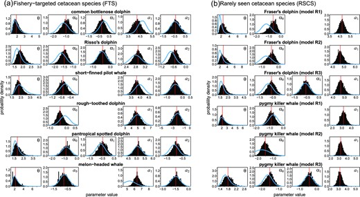
Prior (blue solid lines) and posterior distributions (histograms) of detection function (θ, α0, and α1) and school size regression parameters (a1 and a2).
Block-specific abundances (RSCS)
A total 12 school encounters of Fraser’s dolphins and five school encounters of pygmy killer whales were recorded since 2006. The medians of estimated effective strip half-width (w) of Fraser’s dolphins were 0.76 nmi using model M1 and 0.88 nmi using model M2, respectively (Table 3). The values obtained using model M3 were 0.53 and 0.89 nmi, respectively, for Beaufort scales < 3 and ≥ 3 (Table 3). The medians of the estimated w of pygmy killer whales were 0.66 and 0.28 nmi, respectively, using models M1 and M2, whereas those obtained using model M3 were 0.26 and 0.40 nmi, respectively, for Beaufort scales < 3 and ≥ 3. The median school sizes estimated using a negative binomial distribution were 108.1 (M2) to 111.0 (M1) for Fraser’s dolphins and 24.6 (M3) to 25.2 (M2) (Table 3). The |$\hat{R}$| values for all estimated parameters were smaller than 1.1 (Gelman et al., 2014).
Simple mean of observed school sizes (|${\boldsymbol{\bar{s}}}$|) and posterior medians (and 95% credible intervals) for the important parameters, effective half-width (|${\boldsymbol{\hat{w}}}$|), estimated school size (|${\boldsymbol{\hat{s}}}$|), encounter rate (|${\boldsymbol{\hat{n}}}/{\boldsymbol{L}}$|), and abundance (|${\boldsymbol{\hat{N}}}$|) for two RSCS.
| |${\boldsymbol{\hat{N}}}$| | |||||||||||
|---|---|---|---|---|---|---|---|---|---|---|---|
| Species | Model | Year | |${\boldsymbol{\bar{s}}}$| | |${\boldsymbol{\hat{s}}}$| | |${\boldsymbol{\hat{w}}}$| | A | B | C | D | E | Total |
| Fraser’s dolphin | M1 | 2006–2007 | 106.2 | 111.0 (64.8–208.8) | 0.76 (0.48–1.08) | 648 (77–2191) | 1 351 (150–4 180) | 7 796 (1 404–30 887) | 7 371 (1 719–21 800) | 4 438 (984–13 528) | 22 834 (7 277–61 715) |
| 2014–2015 | 622 (35–2 650) | 1 338 (70–5 173) | 10 567 (2 601–52 115) | 11 105 (2 762–48 436) | 10 832 (2 104–50 495) | 38 206 (13 092–126 347) | |||||
| 2019–2021 | 626 (31–2 642) | 1 868 (322–7 905) | 10 410 (2 589–53 747) | 9 183 (1 542–36 877) | 3 752 (196–15 061) | 28 718 (9 520–92 245) | |||||
| M2 | 2006–2007 | 108.1 (64.4–218.5) | 0.88 (0.63–1.20) | 524 (48–1 913) | 1 050 (89–3 590) | 6 486 (1 128–27 004) | 6 098 (1 478–18 156) | 3 672 (690–11 497) | 18 952 (6 032–52 717) | ||
| 2014–2015 | 491 (22–2 164) | 1 045 (41–4 426) | 9 274 (2 264–48 407) | 9 780 (2 446–41 477) | 9 269 (1 575–45 646) | 33 643 (11 899–112 644) | |||||
| 2019–2021 | 513 (21–2 387) | 1 551 (239–6 684) | 9 148 (2 208–45 334) | 7 614 (1 305–33 273) | 3 039 (138–13 573) | 24 548 (8 523–76 235) | |||||
| M3 | 2006–2007 | 108.4 (64.8–208.5) | 0.89 (0.56–1.37; BF < 3) 0.53 (0.35–0.80; BF ≥ 3) | 731 (69–2 514) | 1 462 (135–4 864) | 6 468 (1 208–28 494) | 8 386 (1 951–25 091) | 5 054 (1 067–16 269) | 23 451 (7 546–64 000) | ||
| 2014–2015 | 675 (31–3 245) | 1 434 (73–6 405) | 12 333 (3 065–60 977) | 13 040 (3 163–58 781) | 9 073 (1 481–44 276) | 41 070 (14 642–134 646) | |||||
| 2019–2021 | 680 (31–2 931) | 2 525 (410–10 363) | 15 221 (3 597–74 186) | 12 342 (2 076–54 054) | 4 212 (186–18 109) | 39 331 (12 965–126 019) | |||||
| Pygmy killer whale | M1 | 2006–2007 | 24.4 | 24.9 (14.7–47.2) | 0.66 (0.47–0.94) | 33 (0–333) | 61 (0–528) | 222 (0–2 919) | 857 (75–4 958) | 283 (0–2 035) | 1 838 (238–7 959) |
| 2014–2015 | 21 (0–414) | 47 (0–688) | 188 (0–3 284) | 209 (0–3 137) | 1 831 (111–18 117) | 3 234 (331–19 294) | |||||
| 2019–2021 | 23 (0–417) | 46 (0–732) | 190 (0–3 188) | 215 (0–3 234) | 923 (57–9 090) | 2 199 (227–11 651) | |||||
| M2 | 2006–2007 | 25.2 (14.9–47.6) | 0.28 (0.18–0.49) | 62 (0–775) | 110 (0–1 220) | 374 (0–6 223) | 1 981 (163–12 391) | 598 (0–4 896) | 4 109 (467–19 042) | ||
| 2014–2015 | 40 (0–1 004) | 80 (0–1 610) | 329 (0–6 827) | 370 (0–7 284) | 4 633 (244–45 615) | 7 590 (696–48 757) | |||||
| 2019–2021 | 39 (0–969) | 80 (0–1 487) | 320 (0–6 545) | 382 (0–7 903) | 2 216 (126–22 322) | 5 009 (493–26 575) | |||||
| M3 | 2006–2007 | 24.6 (14.7–49.0) | 0.26 (0.17–0.40; BF < 3) 0.40 (0.29–0.55; BF ≥ 3) | 60 (0–662) | 121 (0–1 050) | 437 (0–5 772) | 1 527 (148–8 167) | 585 (1–3 812) | 3 466 (458–14 641) | ||
| 2014–2015 | 42 (0–773) | 87 (0–1 400) | 375 (0–6 114) | 375 (0–6 137) | 3 245 (172–29 964) | 6 123 (631–34 018) | |||||
| 2019–2021 | 45 (0–755) | 86 (0–1 477) | 389 (0–6 199) | 414 (0–6 465) | 2 310 (141–23 120) | 5 075 (525–27 720) |
Two |${\boldsymbol{\hat{w}}}$| values were obtained for R3 of both species because covariate of BF was included in the detection functions.
Table 3 summarizes the abundance estimates in respective blocks by three periods, 2006–2007, 2014–2015, and 2019–2021. For the blocks repeatedly surveyed in the successive years (e.g. block C in 2006 and 2007), averaged values were shown as abundance in respective periods. Fraser’s dolphins were more frequently encountered in blocks C and D, whereas no sightings were recorded in block A since 2006 (Figure 2). WAICs were 225.3, 223.9, and 227.5, respectively, for M1–M3. Total abundances estimated by the lowest WAIC model, M2, were 18952 (6032–52717), 33643 (11899–112644), and 24548 (8523–76235) in 2006–2007, 2014–2015, and 2019–2021, respectively. Encounters of pygmy killer whales were concentrated mostly in block E, with the exception of block D in 2007 (Figure 2). Sightings were also recorded in block E exclusively during the latest surveys, in 2019–2021. WAICs of M1–M3 were 79.0, 75.8, and 76.8, respectively. Total abundances estimated by the lowest WAIC model, M2, were 4109 (467–19042), 7590 (696–48757), and 5009 (493–26575) in 2006–2007, 2014–2015, and 2019–2021, respectively.
Abundance trends of FTCS
The exponential population dynamics model was fitted to the abundance estimates with random effects to express spatiotemporal changes in animal distribution. The annual changes in abundance and their percentiles are illustrated in Figure 5. The trends in the total abundance of each species are expressed as a simple exponential form, while the block-specific abundances were fitted well with the original data of abundance estimates using random effects. Abundances estimated by trend model showed much larger variances than original estimates, because additional variances were incorporated into them. Total abundances in 2020 (mid-year of the latest surveys) for common bottlenose dolphins were 49762 (95% CI = 19043–175984 and CVs = 0.67), 194676 (66310–764357 and 0.73) for Risso’s dolphins, 43585 (14274–274897 and 1.15) for short-finned pilot whales, 11127 (2455–129460 and 2.21) for rough-toothed dolphins, 152485 (54797–399938 and 0.53) for pantropical spotted dolphins, and 73412 (23443–231995 and 0.63) for melon-headed whales (Table 4). The median R-values tended to be smaller for common bottlenose dolphins than for other species (Table 4). The probability of |$N_{2020}^{tot}$| to be larger than 95% of |$N_{2006}^{tot}$| (P95) and that of 60% (P60) also tended to be smaller for common bottlenose dolphins (Table 4). PBR was 320 for common bottlenose dolphins, 1187 for Risso’s dolphins, 230 for short-finned pilot whales, 51 for rough-toothed dolphins, 951 for pantropical spotted dolphins, and 442 for melon-headed whales (Table 4).
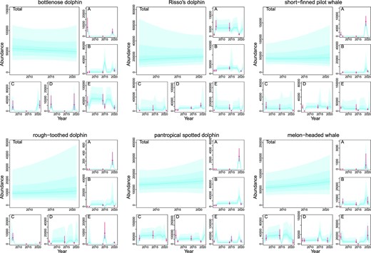
Median and 0.90, 0.75, 0.60, 0,40, 0.25, and 0.10 posterior percentiles of total abundance of six FTCS across the blocks A–E and block-specific abundances by trend model with random effects accounting for spatiotemporal changes in animal distributions. Bars represent the median and 60% CIs of bootstrapped block-specific abundance estimates in 2006, 2007, 2014 and 2015, 2019, 2020, and 2021.
Summary of abundance trend analyses.
| Species | NLL | σ | R | P95 | P60 | |${\boldsymbol{N}}_{2020}^{{\boldsymbol{tot}}}$| | CV | PBR2020 |
|---|---|---|---|---|---|---|---|---|
| Common bottlenose dolphin | 172 (152–19 069) | 9.5 (8–12.8) | 0.99 (0.95–1.04) | 45.9 | 66.2 | 49 762 (19 043–175 984) | 0.67 | 320 |
| Risso’s dolphin | 183 (170–193) | 2 (1.3–3) | 1.04 (0.95–1.04) | 64.8 | 69.8 | 194 676 (66 310–764 357) | 0.73 | 1187 |
| Short-finned pilot whale | 158 (145–6 410) | 9.1 (7.5–14) | 1.02 (0.95–1.04) | 61.6 | 77.6 | 43 585 (14 274–274 897) | 1.15 | 230 |
| Rough-toothed dolphin | 756 (109–14 128) | 9.2 (7.3–11.5) | 1.04 (0.95–1.04) | 69.7 | 80.9 | 11 127 (2 455–129 460) | 2.21 | 51 |
| Pantropical spotted dolphin | 174 (164–5 751) | 4.9 (4–6.3) | 1.02 (0.95–1.04) | 68.2 | 84.3 | 152 485 (54 797–399 938) | 0.53 | 951 |
| Melon-headed whale | 148 (121–11 230) | 6.2 (4.1–12.4) | 1.04 (0.95–1.04) | 79.7 | 92.6 | 73 412 (23 443–231 995) | 0.63 | 442 |
Negative log-likelihood (NLL, median and 95% credible intervals), probability that abundance in 2020 was larger than 95 or 60% of abundance in 2006 (P95 and P60), total abundance in 2020 (|${\boldsymbol{N}}_{2020}^{{\boldsymbol{tot}}}$|), and PBR at 2020.
Discussion
Data-limited abundance estimation for small cetaceans
In 2019–2020, the JAFRACSS small cetacean surveys spent a total of 126 days covering the entire study areas (A–E). Despite such efforts, the number of school sightings did not meet the criterion for robust abundance estimation suggested by Buckland et al. (2001). Coping with such an issue, the Bayesian approach can efficiently incorporate the existing knowledge into a probabilistic form, and update this knowledge as new data become available (Chrysafi and Kuparinen, 2015). Prior distributions for the parameters of detection functions were updated using the dataset obtained in the latest surveys, and these models provided the latest abundance estimates for these data-limited populations. For FTCS, the shapes of the detection function tended not to be largely different from priors for many species (Figure 3), which might indicate that the samples size was too small to update the probability distributions. Specifically, the prior and posterior distributions of parameters were almost identical in the detection function of melon-headed whales (Figure 4). Conversely, considering the relatively large number of school sightings recorded for common bottlenose dolphins, Risso’s dolphins, and short-finned pilot whales, it is possible that the probability distributions obtained from the latest data were actually similar to the previous ones. Regardless of the causes, combining the recent data into the past dataset through Bayesian updating is a reasonable approach, because the past and latest datasets were obtained for the same species and the same geographic ranges and both surveys followed almost the same sampling protocols (e.g. vessel type, height of the observation platform, and binocular magnification, etc.).
The detection functions of the two RSCS were also estimated through Bayesian updating from the prior distributions. However, we borrowed prior information from other small cetacean species; thus, their reliability might be arguable. In the case of Fraser’s dolphins, through Bayesian updating, the shapes of the detection functions were clearly modified from the prior distribution (Figure 3b). WAIC values were smaller in M2, but the posterior medians of effective strip half-width w became not largely different among the models (M1: 0.76, M2: 0.88, M3: 0.89, when Beaufort scale < 3). The abundance estimates tended to be larger in model M3, because the effective half-width was smaller when the Beaufort scale ≥ 3 (median: 0.53). Nevertheless, those differences were not very large. The medians of total abundances estimated by the lowest WAIC model (M2) were 18952 (6032–52717), 33643 (11899–112644), and 24548 (8523–76235) in 2006–2007, 2014–2015, and 2019–2021, respectively (Table 3), which represented relatively small differences from the other models. Conversely, the posterior parameter of detection function did not change largely for pygmy killer whales, suggesting an insufficient sample size for updating the information and for the reliable estimation of the abundance. In fact, the estimated abundance varied substantially among the models. The medians of total abundances by the lowest WAIC model (M2) were 4109 (467–19042), 7590 (696–48757), and 5009 (493–26575) in 2006–2007, 2014–2015, and 2019–2021, respectively, which were about two times larger than estimates by M1 (Table 3).
For both FTCS and RSCS, we assumed perfect detection on a track line [i.e. g(0) = 1], but this assumption might be violated by two primary causes: “availability bias”, which occurs when animals are under the water and “perception bias”, which occurs when animals are available to be seen but missed due to fatigue or any other observation conditions (Laake and Borchers, 2004). Satellite telemetry data for diving behaviour and data from double platform survey will provide information to evaluate availability and perception biases, respectively. JAFRACSS small cetacean survey has not had any protocols to evaluate them, but a few studies from Japanese sighting surveys estimated g(0) (Takahashi, 2019). Okamura et al. (2012) analysed diving and surfacing records of tagged Baird’s beaked whales and estimated g(0) to be 0.78 for a single animal to 0.92 for a school of 30 animals. Using the data from double-platform surveys, Takahashi (2019) estimated g(0) of minke whales to be 0.676 for the top barrel, 0.429 for the independent observer (at a platform lower than the top barrel), and 0.810 for the pooled platforms. Baird’s beaked whales frequently make diving longer than 30 min (Okamura et al., 2012), and Antarctic minke whales have relatively small school size (1–2 of mean school size; Hakamada et al., 2014). On the other hand, the diving depth of delphinids are generally shallow and diving duration is short during the daytime (Scott and Chivers, 2009; Wells et al., 2009; Silva et al., 2016). School size is much larger than baleen whales (Tables 2 and 3). However, even if detection probability on the track line is nearly 1 in fine weather, wind force may additionally affect detectability (Barlow, 2015). Further consideration and data collection on g(0) will be needed for more precise abundance estimation in our future work.
Currently, all six FTCS mentioned above were managed based on PBR (Wade, 1998) in the waters off Japan. Although the government has set annual catch limit for all FTCS, dolphin fisheries remain controversial (Kasuya, 2007; Vail et al., 2020), and stakeholders from different standpoints often have extremely different opinions. Therefore, sharing a more straightforward decision-making process and easy-to-understand scientific information among all stakeholders should be a key to the conservation and management planning of FTCS. In this regard, updating the latest abundance is a core scientific component. Here, we reported an approach to estimate abundance using past information and limited data. This does not mean that revision on the past abundance impedes proper decision-making. Collecting data and updating assessment would be rather appropriate direction in adaptive management (Hilborn and Walters, 1992; Hammond et al., 2021). Standard approach would be combining the data from the past through the latest years and then reanalysing them and updating both the past and latest abundance information (e.g. Kanaji et al., 2018). The present study provides another option of effectively incorporating past information and knowledge into the latest abundance estimation and future modifications in conservation planning. Bayesian estimation has another merit in that it calculates the catch limit, because a lower percentile is usually used for reference abundance (Wade, 1998). Such reference abundance and its uncertainty are more explicitly expressed from the likelihood from joint models of detection probability, school size, and encounter rate (Moore and Barlow, 2011, 2014).
The Japanese government established the Second Basic Plan of Ocean Policy in 2013, which aimed to “collect and compile information about rare marine organisms by assessing endangered marine organisms by the level of their chance of extinction by FY (fiscal year) 2016” (Cabinet Office, Government of Japan, https://www8.cao.go.jp/ocean/policies/plan/plan.html, accessed on 15 May 2023). By adopting this plan, the government released the first edition of the domestic Red List of marine organisms in 2017 (Ministry of the Environment, https://www.env.go.jp/content/000037610.pdf, accessed on 15 May 2023). A total 29 small odontocetes were assessed in this list, but the assessments of many species relied on limited biological information and empirical rules because of the lack of quantitative information. Finally, all small cetacean species were categorized as “unranked” based on qualitative assessments. Such a data-limited situation has been commonly recognized in the IUCN Red List, particularly in less-frequently observed oceanic cetaceans. For example, Fraser’s dolphins have been considered as “rare species” in the waters off Japan because of the infrequency of their encounters (Mammal Society of Japan, 1997). We tested the data-limited abundance estimation for two RSCS. All three models with different priors estimated several tens of thousands of Fraser’s dolphins inhabiting the waters off Japan (Table 3), which indicated that the current population size was much larger than previously believed. Conversely, a mean abundance of pygmy killer whales of only several thousands was estimated using three models (Table 3). This abundance was an order smaller than that of Fraser’s dolphins, and their habitat was limited to relatively small areas of block E and the southwest part of block D. Although uncertainty still remains, the estimates provided here are undoubtedly important for assessing the population status of RSCS.
Abundance trends and conservation implications
It has been widely recognized that time series of abundance and the trends derived from the time series are fundamental for assessing and predicting the current and future population status of various species (Hilborn and Walters, 1992). However, such information was often ineffective to identify at-risk stocks, because the statistical power to detect trends in abundance was low when using the available datasets for many marine mammal populations (Taylor et al., 2007). Traditionally, hypotheses-based statistical analyses are employed to detect abundance trends (e.g. Kanaji et al., 2011); however, this approach often failed because of the large uncertainty in the abundance estimates and infrequent surveys (Taylor et al., 2007). The simulation-based approach presented here provided important information on the status in population abundance over the past 15 years.
The method to model the abundance trends was inspired by an approach developed by Skaug et al. (2004), in which random-effects model was fitted to the line-transect survey data for Atlantic minke whales. Their datasets did not have blocks with no sightings, and thus the estimated additional variance parameter was successfully estimated with reasonably small value (|$\hat{\sigma } = 0.22$|) from repeated surveys in the same block (Skaug et al., 2004). On the other hand, several species had zero abundance estimates in specific blocks and years in our previous estimates (Kanaji et al., 2018). Zero abundances were dealt with by a mixture of Poisson distribution through random-effects modelling, but it eventually resulted in large additional variance estimates (e.g. |$\hat{\sigma } = 9.5$| for common bottlenose dolphins; Table 4). In spite of these caveats, overall, trend model was fitted well to the abundance data and uncertainty in abundance estimates were sufficiently considered by random effects accounting for the interannual changes in animal distributions (Table 4 and Figure 5). The R tended to be smaller for common bottlenose dolphins than for the other species (Table 4). Regarding the estimated population trends, the posterior odds of the latest abundance (|$N_{2020}^{tot}$|) being below or above the abundance at the starting year (|$N_{2006}^{tot}$|) is expected to be 50% if the abundance remains constant during the study period. P95 of common bottlenose dolphins was smaller than 50%, and P60 also showed relatively smaller values for the species. Among six FTCS, rough-toothed dolphins, pantropical spotted dolphins, and melon-headed whales were oceanic species, and mainly inhabit offshore waters and around oceanic islands (Kanaji et al., 2017). Given their habitat being not much susceptive to human-caused disturbances and being not main target by dolphin fisheries, abrupt population reduction between the past 15 years seems unreasonable. On the other hand, these results support our previous recognition that the abundance of common bottlenose dolphins has been gradually decreasing over the past few decades (Kanaji et al., 2021). Conversely, the population size of Risso’s dolphins has been increasing in recent years (Kanaji and Gerrodette, 2020; Kanaji et al., 2021). Currently, annual catch limits for these six FTCS are 500 for common bottlenose dolphins, 460 for Risso’s dolphins, 168 for short-finned pilot whales, 40 for rough-toothed dolphins, 470 for pantropical spotted dolphins, and 363 for melon-headed whales (based on the amendment in 2017; Yoshida, 2019). Total (combined) abundance estimates tended to be larger when trend model was applied than those from simple sum of the abundance estimates from different blocks/years (Tables 2 and 4). Trend model incorporated additional variances into the former estimates, thereby resulting in similar PBRs with the latter approach except for Risso’s dolphins and pantropical spotted dolphins. For both results, the current catch limit largely exceeds our PBR estimates only for common bottlenose dolphins, although the annual catch in the past 10 years from 2011 to 2020 were 111–262, which has not exceeded them.
What lessons did we learn from this modelling study, and how do we change or modify the conservation measures for FTCS and RSCS in the waters off Japan? First, we detected the species of greater concern in terms of population trends. As a result of the three types of trend analyses, only the common bottlenose dolphin showed a decreasing trend in abundance. These results would help prioritize our conservation efforts. Second, many RSCS have not been covered by stock assessments in Japan, whereas there is currently an increased demand for assessment of population statuses even for non-fishery–targeted cetaceans. Our approach may be applicable to many other species with no quantitative information to date. For example, information and datasets for the well-studied and fishery-targeted beaked whales (Miyashita, 1986; Kasuya and Miyashita, 1997; Okamura et al., 2012) may help assess the population status of the other beaked whale species without sufficiently quantitative information. Third, the present study indicated that distribution changes likely affected assessment output, particularly for species inhabiting the dynamic ocean environment. In the California current system, population dynamics models combined with habitat modelling substantially improved the precision of the estimations of abundances and their trends (Boyd et al., 2018; Boyd and Punt, 2021). Similarly, cetacean habitats likely change on a yearly basis according to the path patterns of Kuroshio Current off the coast of Japan (Kanaji and Gerrodette, 2020). Habitat modelling can also deal more explicitly with spatial structures of animal distributions by spatial random effect (e.g. intrinsic conditional autoregressive, iCAR; Blangiardo and Cameletti, 2015). However, habitat models generally require a greater number of parameters to be estimated, and sufficient sample size (≥30) is required to estimate habitat with high precision (Wisz et al., 2008). How do we model spatial structures for data-limited cetaceans is a challenge for the future, but our approach might be preferred at this stage because small samples might not fit well to the spatial modelling of environmental relationships. Moreover, continuing comprehensive sighting surveys, such as the JAFRACCS programmes, and updating the information on the current population status, are definitely our responsibility as cetacean researchers. We believe that our survey programme and analytical approaches will improve the management and conservation schemes in Japan and provide ideas for conserving cetacean populations in many other regions.
Acknowledgements
The authors are grateful to the team involved in the JAFRACSS programme. This manuscript greatly benefitted from the comments of the editor, two anonymous reviewers and Matthieu Authier. Last, we would like to express our gratitude and respect to the late Hideyoshi Yoshida. Yoshida had led Cetacean Research Group in Japan Fisheries Research and Education Agency for long years and suddenly passed away in May of 2023. This study would not be possible without his guidance and support.
Funding
The collection of data used in this study was conducted as a part of the research and assessment programme for fisheries resources, the Fisheries Agency of Japan. This study was also financially supported by the Japan Fisheries Research and Education Agency and the Institute of Cetacean Research.
Conflict of interest statement
The authors declare no conflicts of interest.
Author contributions
YK: conceptualization, formal analysis, methodology, software, and writing–original draft; HS: data curation and investigation; TH: validation and writing–review and editing; and HO: conceptualization, methodology, software, and writing–review and editing. All authors have read the manuscript and agreed to publish it.
Data availability statement
All relevant data and software code are publicly available in the supporting information files (Appendix 3).
