


Abstract
Atlantic halibut (Hippoglossus hippoglossus) support an economically important fishery on the eastern coast of Canada. Like other species that are not well sampled by trawl surveys, halibut in this area are monitored using longline surveys. These surveys present challenges that can make obtaining indices of abundance difficult. Issues include gear saturation, which can result in a non-linear relationship between catch per unit effort and local abundance. The current approach to obtain a relative index consists of fitting a multinomial exponential model to a subset of hooks from each survey station. While this approach accounts for hook competition, it does not account for the presence of spatial patterns. We therefore extend the multinomial exponential model to include spatial random fields for both Atlantic halibut and non-target species, set-specific soak time, and data from the hooks. Furthermore, we propose a method for aggregating the resulting spatially varying indices to obtain an annual index for the entirety of the modelled area. This novel approach identifies Atlantic halibut hotspots in multiple years, while simultaneously providing relative abundance indices for 2017 through 2020. These outcomes demonstrate the widespread applicability of our methods for improving the scientific advice upon which fisheries management decisions are based.
Introduction
The management of economically important fisheries is a difficult and laborious process where fisheries scientists must extract the best possible indicators of population size and abundance from noisy fisheries data. The resulting estimates and their associated errors are used by fisheries managers to develop fishing targets aimed at ensuring the sustainability of both the exploited population and the fishery exploiting it. The difficulty in analyzing fisheries data stems from the fact that they are typically noisy (Punt et al., 2000), contain complex non-linear relationships (e.g. Froese, 2006; Morson et al., 2018), and often follow non-Gaussian distributions (Martin et al., 2005; Cressie et al., 2009; Etienne et al., 2013). While various methods have been developed to obtain reliable indices of population abundance (e.g. through better stratification approaches and sampling designs; Smith, 1996; Kimura and Somerton, 2006), these can be harder to apply to data from non-trawl surveys such as longline surveys.
The main difficulty in assessing longline survey data is that the raw data are not well captured by the usual continuous distributions employed to obtain indices of abundance (e.g. lognormal distributions; Hansell et al., 2020). Many approaches have been proposed to attempt to deal with this issue, mostly revolving around standardizing the raw data into catch rates and catch per unit effort (CPUE), which are defined as the average number of fish of the target species caught per hook and minute of soak time (Etienne et al., 2013). For the Atlantic halibut (Hippoglossus hippoglossus) fishery on the eastern coast of Canada, initial efforts saw design-based approaches used to obtain stratified weighted mean catch rates. Further improvements were made to better standardize these catch rates by combining a design-based approach with a statistical modelling framework that used a negative binomial generalized linear model (GLM) (Trzcinski et al., 2009; den Heyer et al., 2015a). While these innovations led to significant improvements, other issues were identified that could potentially bias these abundance indices.
Previously available methods were not able to account for the impacts of gear saturation and competition for baited hooks within and between species (Etienne et al., 2013; Smith, 2016), and these methods further assumed that all hooks on a longline are capable of catching fish for the duration of the line’s deployment. They also ignored unbaited empty hooks that would not reliably catch fish in the same way as baited hooks. Any one of these issues would result in decreased efficiency of fishing effort while also leading to bias in estimated indices of abundance (Beverton and Holt, 1957). A solution to account for competition between target and non-target species for baited hooks as well as the treatment of empty-unbaited hooks is to use a multinomial exponential model (MEM), originally proposed by Rothschild (1967) and modified by Etienne et al. (2013). While MEM performs well in its standard formulation (Etienne et al., 2013), it does not account for spatial patterns in the data. Given the scale and environmental complexity of fisheries management units for Atlantic halibut in general, the indices produced using the MEM would no doubt benefit from the inclusion of spatial effects to account for possible spatial patterns in fish abundance.
Models that include spatially correlated random effects are becoming increasingly popular in fisheries science. These models have been used to standardize CPUE data and improve estimated abundance indices (Nishida and Chen, 2004; Thorson and Ward, 2013; Shelton et al., 2014), and predict bycatch hotspots (Cosandey-Godin et al., 2015; Yan et al., 2021). Utilizing geostatistics, they incorporate spatial structure in the model residuals (Ciannelli et al., 2008) to capture the latent spatial variability not explained by the covariates included in the model framework (Cadigan et al., 2017; Stock et al., 2020). These methods have been applied to both invertebrate and groundfish species (e.g. Thorson et al.,2015; McDonald et al., 2021), but for many key species these methods have not been tested.
In this paper, we propose a novel statistical framework in which a multinomial model for hook competition (MEM) is integrated with a spatial model for station-specific data (MEMSpa). We include Gaussian random fields as spatial random effects for both target and non-target species to infer their underlying population distributions from survey data. We undertake a simulation study to explore the estimability of this novel approach under two different scenarios. We then fit our new model to data from the Scotian Shelf and Southern Grand Banks Atlantic halibut longline survey, which provides an index of abundance for one of the most valuable groundfish fisheries in eastern Canada. As this new model allows the estimation of relative abundance indices at each survey station, we aim to evaluate the effectiveness of the current stratification scheme for the area, while simultaneously presenting a method to estimate an aggregate overall abundance index for the entire region.
Material and methods
Data description
Atlantic halibut is an economically important demersal flatfish that is distributed on the continental shelf and along the shelf edge across the North Atlantic Ocean and in part of the Arctic Ocean. There are two Atlantic halibut management units in Canadian waters, namely the Scotian Shelf and southern Grand Banks (North Atlantic Fisheries Organization [NAFO] Divisions 3NOPs4VWX5Zc), and the Gulf of St. Lawrence (4RST). We focus on 3NOPs4VWX5Zc (Figure 1), where the biomass of exploitable halibut has been monitored by a Fisheries and Oceans Canada-Industry collaborative longline survey since 1998. The longline survey was established because Atlantic halibut, as the largest flatfish species, were not well sampled by research vessel (RV) trawl surveys that provide the primary fishery-independent abundance indices for other groundfish stocks in Atlantic Canada (Zwanenburg et al., 2003).
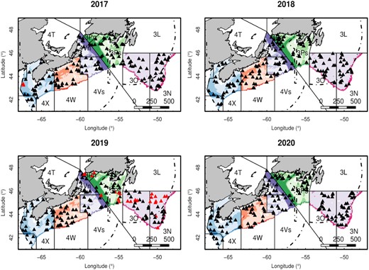
Locations of longline survey stations in 2017, 2018, 2019, and 2020. The 3NOPs4VWX5Zc Atlantic halibut stock survey area is denoted by the coloured area, with five area strata: 4X5YX (blue), 4W (orange), 4V (purple), 3P (green), and 3NO (red), and three depth strata: 30–130 m (light colour), 131–250 m (medium colour), and 251–750 m (dark colour). NAFO subdivsions are labelled, and separated by solid lines. The exclusive economic zones of Canada and France are shown with dashed lines. NAFO subdivision 3Pn is not part of the stock area, but is currently included in the survey. Black triangles are the successfully completed stations and red triangles are the incomplete stations. Scale bar is in kilometres.
The longline survey provides internally consistent estimates of Atlantic halibut relative abundance and does not suffer from the high variability observed in the RV survey results because it has a much higher catchability for Atlantic halibut (Zwanenburg et al., 2003). Longlines are placed at the seafloor (demersal longlines) to catch bottom-dwelling fish such as halibut. As their name implies, longlines consist of a long mainline to which baited hooks are attached at regular intervals by way of a branch line or gangion. The Atlantic halibut longline survey is completed by commercial fishers with at-sea observers collecting data and ensuring compliance to survey protocols. While the survey was originally stratified into areas of low, medium, and high catch rates based on data from commercial fishing logs (1995–1997) (Zwanenburg and Wilson, 2000), a new stratified random survey design was introduced in 2017 to expand geographic coverage, standardize fishing protocols, and improve data collection (Smith, 2016; Cox et al., 2018). Here we focus on the data from this new stratification scheme (2017–2020).
The stratified random survey area is divided into five area strata (NAFO Divsions 4X5YZ, 4W, 4V, 3P, and 3NO), each with three depth strata (30–130, 131–250, and 251–750 m). While the management area does not include 3Pn, it is included in the survey. The depth stratum boundaries (30–750 m) were chosen because they contain most of the fishing sets and Atlantic halibut habitat (Cox et al., 2018). Depth strata were selected based on exploratory analyses of catch rates by depth using fixed stations and commercial index sets from the original Atlantic halibut survey. The depth stratification can also provide a proxy for temperature and some bottom habitat information. Survey stations are randomly assigned to strata with the number of stations allocated proportionally to the size of each stratum. A total of 150 stations were allocated in 2017, and 153 stations were allocated in each year from 2018 to 2020 (Figure 1). Additional stations were added to strata that had contained only two stations in an effort to reduce the probability of unfished strata or strata with only one station fished.
Gear design and fishing procedures were standardized. Each set had 1 000 baited hooks, with gangions spaced 4.6–5.5 m apart for a total length of gear between 4.6 and 5.5 km. Size 15 circle hooks were baited with pieces of herring (125–200 g) and the gear was set for between 6 and 12 h. In area strata 4X5YZ, 4W, and 4V, a sinking mainline was used, while in area strata 3P and 3NO a buoyant polypropylene rope was used to which (454–1815 g; 1–4 lb) weights are attached. The more buoyant line was thought to mitigate against bait loss in some bottom types (mud versus rock). Gear type is therefore expected to impact the performance of the gear; however, the hook occupancy data (empty with bait versus empty with no bait) will also reflect the differences in the gear. Hook condition data were collected by trained observers who monitor the longline and record location, depth, and time for the setting of the gear and the haul back. For each longline, every Atlantic halibut was counted, its length measured, and although our work here only focuses on the number of fish, its weight was estimated. The total kept and discarded catch (number and weight) of other species was also estimated for each longline. [see den Heyer et al. (2015b) for details].
An unpublished internal pilot study, and subsequent mathematical modelling, indicated observing hook condition in a subset of 300 hooks is sufficient to be representative of the entire 1 000 hooks. Hook condition is assessed and recorded from 300 hooks for each 1 000 hook longline set. For each set, the 300–hook sample consists of 10 subsamples of 30 consecutive hooks, wherein these subsamples are taken roughly every 100 hooks. This results in sampling throughout the longline and avoids bias associated with sampling only the beginning, end, or middle of the set. The condition of each hook at retrieval in the hook occupancy sample was recorded, by assessing whether the hook was baited, empty, or with a catch and the species caught. For each longline, we obtained counts of hooks with target catch, hooks with non-target catch, empty-baited hooks, empty-unbaited hooks, and broken hooks. While only a subset of the 1 000 hooks (per set) had every hook status recorded, there is still information available for the rest of the set that can be incorporated in the model, namely, the number of target species caught (halibut), the estimated number of non-target species caught, and the number of empty hooks (which could be unbaited, baited, or broken). Temperature recorders (VEMCO minilogs) were attached to most longlines and information on temperature, depth, and soak time for each longline set is also included along with other essential information (see Supplementary Section S2 for additional details).
Multinomial exponential model
MEM
However, it is common for some hooks to return with no bait and no fish at the end of soak time in longline fishing and surveys. The original MEM was therefore modified by Etienne et al. (2013) to account for these empty-unbaited hooks (which also include broken or missing hooks) so that more precise estimates of indices of relative abundance could be obtained. It is assumed that all empty-unbaited hooks are caused by the escape of fish (i.e. the fish “steals” the bait).
This model was developed in the llsurv package in R (R Core Team, 2021) for the Atlantic halibut Scotian Shelf and Southern Grand Banks Fisheries and Oceans Canada-industry collaborative longline surveys (Smith, 2016) using explicit formulae to compute maximum likelihood estimates of the multinomial model parameters in order to estimate relative abundance. In this formulation, it was assumed that Si was constant across all sets by using the mean soak time.
Spatial multinomial exponential model (MEMSpa)
The Matérn model is identifiable, although joint estimates are generally highly variable (Zhang, 2004), and the common approach to fix ν = 1 (Lindgren et al., 2011; Thorson et al., 2015) is also used here. The so-called practical, effective, or decorrelation range, which is the distance at which the correlation of the random field decreases to 0.05, equals 3ϕ for ν = 1.
We projected the longitude and latitude of the survey stations using the WGS84––UTM zone 20N coordinate reference system into eastings and northings in kilometers. Furthermore, we re-scaled the eastings and northings to a range between zero and one for numerical stability.
The model is formulated in C++ and then optimized in R using the TMB package (Kristensen et al., 2016). The TMB package helps to speed up the optimization by taking advantage of automatic differentiation and the Laplace approximation for integrating over random effects (see Kristensen et al., 2016 for details).
One advantage of utilizing classical geostatistical methods as we do here is the ability to predict the abundance index across the entire modelled area through the use of kriging. Kriging is a method of spatial interpolation by which the interpolated values are modelled with a Gaussian process governed by a prior covariance function (Gelfand et al., 2010). The random fields for target species |$\omega _{T}(\mathbf {s})$| and non-target species |$\omega _{NT}(\mathbf {s})$| can therefore be interpolated over a grid covering the modelled area. For the halibut survey, this grid is made up of 4 × 4 km blocks, with the interpolation done at the centre of each block (Cox et al., 2018).
Product likelihood approach
Aggregated relative abundance indices
MEMSpa provides estimated halibut abundance indices at each survey station, with an extra step required to obtain a single index of abundance for the entire area management. While two different approaches were explored for this purpose, we settled on a Dirichlet method (see Supplementary Figure S4 and further details on the alternative explicit method).
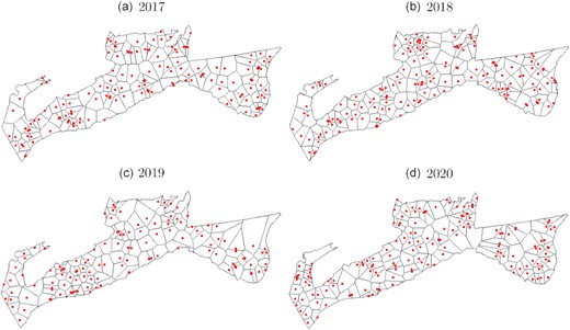
The survey stations and the Dirichlet tessellation for 2017, 2018, 2019, and 2020.
Simulation experiments
Two simulation experiments were conducted to assess the estimability and identifiability of MEMSpa using the product likelihood approach, with the focus on parameter estimation and the estimation of abundance indices. Both data simulation and model fitting were performed using TMB, where data are simulated from Equations 6–10. The first experiment modelled a higher mean probability of capture for the target than the non-target species, but both had relatively high probability of capture (set respectively at 2×10⁻³ and 1×10⁻³). The second examines how the MEMSpa estimation performs when the target species has a very low probability of capture relative to that of the non-target species (set respectively at 1.88×10⁻⁵ and 1.94×10⁻³). The goal of these simulations was to see if a fish being a target or non-target has any effect on parameter estimability, and determine if fitting problems are introduced when one of them has a very low probability of capture.
For each experiment, 500 datasets with 150 observations of 1 000 hooks were simulated with ν fixed at 1 (300 hooks were simulated from the full multinomial model and 700 from the reduced one). As the soak time and the distance between each station are not explicitly modelled in Equations 6–10, they needed to be simulated separately. A unitless simulation square with an area of 9.3262 was created to most closely mirror the unitless standardized distances in the 2017 halibut survey data. The locations of the observations were randomly distributed across the square to obtain the distances between them. The soak times were simulated from a lognormal distribution with a mean of 450 min (7.5 h) on the natural scale and a standard deviation of 0.2 on the log scale.
True values for the parameters are provided in Table 1. The maximization of the likelihood was performed using the quasi-Newton optimizer nlminb in R.
Parameter values used for the two simulation experiments.
| Parameter | Experiment 1 | Experiment 2 |
|---|---|---|
| βT | 2×10⁻³ | 1.88×10⁻⁵ |
| βNT | 1×10⁻³ | 1.94×10⁻³ |
| pNT | 0.8795 | 0.8795 |
| ϕT | 0.07 | 0.07 |
| ϕNT | 0.1 | 0.1 |
| |$\sigma _T^2$| | 3 | 3 |
| |$\sigma _{NT}^2$| | 1.5 | 1.5 |
| Parameter | Experiment 1 | Experiment 2 |
|---|---|---|
| βT | 2×10⁻³ | 1.88×10⁻⁵ |
| βNT | 1×10⁻³ | 1.94×10⁻³ |
| pNT | 0.8795 | 0.8795 |
| ϕT | 0.07 | 0.07 |
| ϕNT | 0.1 | 0.1 |
| |$\sigma _T^2$| | 3 | 3 |
| |$\sigma _{NT}^2$| | 1.5 | 1.5 |
Halibut survey
To test the performance of MEMSpa with real data, it was fitted separately to data from the halibut survey in NAFO division 3NOPs4VWX5Zc (Figure 1) for 2017, 2018, 2019, and 2020 using TMB. Since the total number of non-target fish caught was estimated separately, there are stations for which the sum of the number of target and non-target species caught was >1 000 (six stations for 2017, three stations for 2018, four stations for 2019, and three for 2020). These stations were therefore dropped. A further two stations were dropped in 2017 because fewer than 30 hooks were recorded, which would make these stations unreliable. This resulted in a total number of stations equal to 141, 150, 123, and 148 for each respective year. As is done for the simulations, the maximization of the likelihood was performed using the quasi-Newton optimizer nlminb in R. Anonymized data alongside model code is available online at github.com/RaphMcDo/MEMSpa-Halibut.
Results
Simulation experiment
For Experiment 1, 499 fits successfully converged and 1 failed to converge, while for Experiment 2, all 500 fits converged. The distribution of parameter estimates (Figure 3) was centred around the true values, implying no evidence of bias.
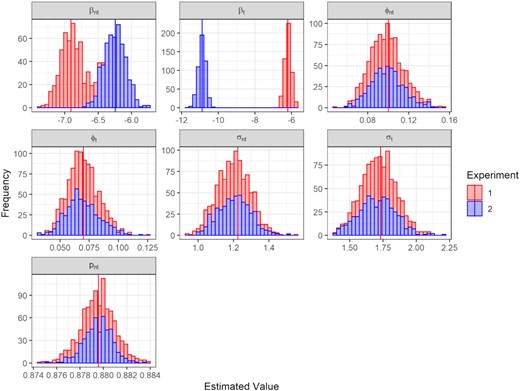
Histograms of parameter estimates from Experiment 1 in red and Experiment 2 in blue (vertical lines denote the true value for each experiment).
When both target and non-target species have relatively high probability of capture as in Experiment 1 (set respectively at 2×10⁻³ and 1×10⁻³), indices of abundance were very well estimated (Figure 4, left panel) with over 86% of estimates within 25% of the true value. However, when the target species had a much lower chance of capture as in Experiment 2 (set at 1.88×10⁻⁵), the model estimates were less precise (Figure 4, right panel), with a little under 50% of the estimates within 25% of the real value for the target species. This indicated that MEMSpa had a greater probability of being further away from the real value when the abundance of the target species is low (distributed around 1.88×10⁻⁵ as in Experiment 2) than high (distributed around 2×10⁻³ as in Experiment 1), but that an overall mean index should still be accurate as the indices were centred at the correct values. Furthermore, this higher variability did not appear to impact the estimation of parameters, spatial or otherwise (Figure 3).
![Histograms of percent differences between estimated relative indices of abundance [λT(si) and λNT(si)] and their true values (target species in red, non-target species in blue) for Experiment 1 (left panel) and Experiment 2 (right panel). Outliers are not shown in the figure for visualization purposes (<0.5% of the runs for Experiment 1 and about 2.8% for Experiment 2).](https://oup.silverchair-cdn.com/oup/backfile/Content_public/Journal/icesjms/79/6/10.1093_icesjms_fsac132/2/m_fsac132fig4.jpeg?Expires=1749854820&Signature=kBe46ECzP9IVtwmQIGF0kxe2Um0NFFJpwUxrJt2US5uHNM-knPHxFPDikvPOXjZTuANglMJPiLRmi~hZRDjikCAV7DCExSwsB4WQKQo9-prFOKqzn-EIsfxUkFALEfFTEURUi51zaPiTgmM0BVvPKGGXzEqRNszttYqU4Dt21FhKFfj7RvCDfZP9U-iJffVhkJIi0yM9B0~-G~sgsO8KhKKuaHGI9Vl~5H9ZeRNUu0jQkLu04en5VS1MP0AbsdANUphGZwQiZVgLjvoY9BBi74CHw~2JNPRo4c2g8JmSCY3QLskqD2ZZ~A-XCFzQn609UXmoqWhiDjCZH8u0-VPs-w__&Key-Pair-Id=APKAIE5G5CRDK6RD3PGA)
Histograms of percent differences between estimated relative indices of abundance [λT(si) and λNT(si)] and their true values (target species in red, non-target species in blue) for Experiment 1 (left panel) and Experiment 2 (right panel). Outliers are not shown in the figure for visualization purposes (<0.5% of the runs for Experiment 1 and about 2.8% for Experiment 2).
Halibut survey
All four model fits (one for each year) successfully converged with parameter estimates shown in Table 2.
Estimated parameters with corresponding standard error in parentheses for MEMSpa from 2017 to 2020.
| Parameter | 2017 | 2018 | 2019 | 2020 |
|---|---|---|---|---|
| βT | −12.303 (0.253) | −11.917 (0.291) | −12.765 (0.415) | −12.341 (0.276) |
| βNT | −6.252 (0.185) | −6.208 (0.118) | −6.050 (0.144) | −6.297 (0.140) |
| pNT | 0.8799 (0.0011) | 0.8992 (0.0010) | 0.9045 (0.0011) | 0.9138 (0.0010) |
| ϕT | 0.0308 (0.0108) | 0.0840 (0.0174) | 0.0641 (0.0161) | 0.0611 (0.0147) |
| ϕNT | 0.0870 (0.0123) | 0.0628 (0.0092) | 0.0569 (0.0104) | 0.0870 (0.0117) |
| |$\sigma _T^2$| | 4.485 (0.877) | 3.557 (0.723) | 6.936 (1.636) | 3.780 (0.806) |
| |$\sigma _{NT}^2$| | 1.518 (0.242) | 0.969 (0.132) | 1.451 (0.212) | 0.867 (0.133) |
The effective ranges for target species calculated from the ϕT parameters (3ϕ) re-transformed to interpretable units (Table 2) were about 31 km for 2017, 79 km for 2018, 60 km for 2019, and 62 km in 2020. As these are decorrelation ranges, they indicate how far apart two points need to be for correlation to cease and hence are suggestive of the size of hotspots for target species. Beyond these distances, the correlation becomes negligible (<0.05). For non-target species, the practical ranges were about 87, 59, 54, and 88 km between 2017 and 2020. The estimates of the other parameters were generally similar across years, with the exception of |$\sigma _T^2$|, which appeared to be higher in 2019 than the other years. The large |$\sigma _T^2$| was most likely the result of the highest halibut catch in the 700–hook dataset for 2019 (104 halibuts) being more than twice the highest catch in all other years.
The estimated relative abundance indices for Atlantic halibut tended to be larger in the shallow areas for 4X5YZ, specifically in the 30–130 m depth stratum (Figure 5). However, the indices appeared to be higher in deeper areas for 4W and slightly higher in the middle depths for 4V. A temporal shift in depth strata with the highest abundance was seen in area 3P, where there was no appreciable difference between depth strata in 2017 and 2018, but the index dropped in the middle depths in 2019 and 2020 (Figure 5). A similar temporal shift in the middle depths was also present in area 3NO, although the highest index was always in the deepest stratum.
![Boxplots of relative abundance indices of target species [λT(si)] on log scale obtained using our spatial model for 2017, 2018, 2019, and 2020. The indices are estimated at each survey station and classified by strata [NAFO Divisions: 4X5YZ, 4W, 4V, 3P, and 3NO; and depth strata: 1 (30–130 m), 2 (131–250 m), and 3 (251–750 m)]. Colours correspond to those in Figure 1.](https://oup.silverchair-cdn.com/oup/backfile/Content_public/Journal/icesjms/79/6/10.1093_icesjms_fsac132/2/m_fsac132fig5.jpeg?Expires=1749854820&Signature=2YUCFtNBdENA5F8siwX-7lnSbNwlRMwyfg6VTsqwnB3Ofr4zzXSJaUJsqi0WJwTJpX44OFi7oKV-H2j7Cm8MqMQqdmZNjRFDvmOZICswDk4qzribTdxWuvku1wBqqDcSOvPjnhMySYLUuVUCDUM9uDPeYHmA78gArT~8YyZqoWWJgc1vxDKz7wgG4m6MTSs0s412Olol4WRVcYG8qI-t4t4bXKgTvgnlsQcqiSNreDsmysX4ECXGXXy0-Q-J9jkWiX1YOjaSIJjnMGnn6By4zoKO-3PpkktlZvL5Ay9UYAwuMI4QAUNLwtk2BFsmzPEcsVI6Ev7np81OI0gfYrng8A__&Key-Pair-Id=APKAIE5G5CRDK6RD3PGA)
Boxplots of relative abundance indices of target species [λT(si)] on log scale obtained using our spatial model for 2017, 2018, 2019, and 2020. The indices are estimated at each survey station and classified by strata [NAFO Divisions: 4X5YZ, 4W, 4V, 3P, and 3NO; and depth strata: 1 (30–130 m), 2 (131–250 m), and 3 (251–750 m)]. Colours correspond to those in Figure 1.
Looking at the overall modelled area spatially, there were only a few recurring areas where halibut appeared to be routinely found at higher abundance in all 4 years (Figure 6): off the south-western tip of Nova Scotia in NAFO division 4X, near the edge of the 4W division south of central Nova Scotia, and around the Laurentian Channel in the middle of the modelled area going up to the Gulf of St. Lawrence (mostly in 3Ps). Temporally, one could see a change in the eastern portion of the area in 3O and 3N where very few halibut were caught in 2020 even if previous years sometimes saw a few good hauls. For the non-target species (Figure 7), the largest abundances were observed on the western edge of the survey area towards the Gulf of Maine and the Bay of Fundy in 4X as well as areas near the Laurentian Channel in 3Ps and 3Pn. While these hotspots did not perfectly overlap with the halibut hotspots, they are very close to one another.
![Estimated relative abundance index for target species [λT(si)] on the log scale in all Dirichlet tiles between 2017 and 2020.](https://oup.silverchair-cdn.com/oup/backfile/Content_public/Journal/icesjms/79/6/10.1093_icesjms_fsac132/2/m_fsac132fig6.jpeg?Expires=1749854820&Signature=WSYIplUAbfy-cBQVaXccVn7frs4m58Fh7ETlxjbMeufR8PWHRY0icUmalow9A~C-8LDbGZ0WnAnsujCB5NWC-~33iHDVrAhybVcEIIk5Xn98VNyjU7mOiDAX5og7j4xX~IbAHjYHHsLOi3lZ8ueukCDS7NfHE-8N9R74tUjUq48Skiu1SG94t6pxdEeDgSuLQzpttPFUl2cMVMbl0H3v~51I4rgHyItwvoxG1zX5vVd9X~gde8lZh7XovQ446SxSuUBVVzcWX61JrYpZXjks~6u5lcBXQi-nNsG-RoKByT~1aNaHZ6gmW24p5i1QH047sM8NrlKTRPfXAF-2S1tORw__&Key-Pair-Id=APKAIE5G5CRDK6RD3PGA)
Estimated relative abundance index for target species [λT(si)] on the log scale in all Dirichlet tiles between 2017 and 2020.
![Estimated relative abundance index for non-target species [λNT(si)] on the log scale in all Dirichlet tiles between 2017 and 2020.](https://oup.silverchair-cdn.com/oup/backfile/Content_public/Journal/icesjms/79/6/10.1093_icesjms_fsac132/2/m_fsac132fig7.jpeg?Expires=1749854820&Signature=q-aJzvf9l56EfjIJ~l3oyNc3qg~qDeefepkW5~Ptr2R1sqxOfWDPWVOYtiKNwpEWesVHXwAwzKcXOXFLn0OAoHoXa2Ln8WOpEUhMqKkp4dSvLriiLSipgNNe3OpHz4xctROObXIifb~8LvWNvT5vJtCiblYOHd~yU1JHSbfo8XvtBNgyMhOVHLl3wVgYQcrmCtz66Fc5WI7Fom1oIQFhOltcuZSOI9ikmd0yERQ3-bP8ST~SYWJ5dtLMcWldoaBW2tOZpFvsew5H2rZ9i~qjmgJZQuj3S~3fyGQ0W8oP5UNe-5XAsuHrhJ7yi6zjxIDaQSCK5V2nr3Fns1waZklIaQ__&Key-Pair-Id=APKAIE5G5CRDK6RD3PGA)
Estimated relative abundance index for non-target species [λNT(si)] on the log scale in all Dirichlet tiles between 2017 and 2020.
The estimated indices for the entire area from the MEMSpa and MEM fits generally agreed on the patterns of change, meaning both indicated similar trends from one year to another (single exception being the non-target index in 2018; Figure 8). MEMSpa always estimated the index at a higher value than the non-spatial MEM. This behavior was caused by two things. First, the inclusion of spatial effects in MEMSpa actually reduced the expected index (for example, βt is −12.303 in 2017 for MEMSpa but it is −10.882 in the same year for the MEM) but allowed the model to better account for a lot of the station-specific variability and have station-specific indices, which could be significantly higher than the aggregated index (see Figure 6). This was then combined with our spatially weighted average approach to aggregation, where the stations with higher indices tend to cover relatively large areas and therefore were more heavily weighted than with the MEM (see Figure 6).
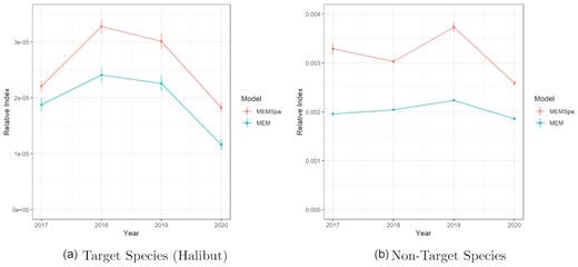
Estimated abundance indices (|$\bar{\lambda }_T$| and |$\bar{\lambda }_{NT}$| for MEMSpa, λT and λNT for the MEM) for target and non-target species for the entirety of the modelled area from fitting MEMSpa and MEM to data from 2017 to 2020. The error bars represent ±1 standard error (error bars are present in panel (b) for the MEM; they are simply extremely small).
Discussion
The creation of MEMSpa has led to the successful integration of previous MEM models accounting for hook competition with geostatistical approaches that can incorporate spatial structure. The resulting station-level and overarching indices along with their corresponding standard errors were better able to capture the latent spatial patterns and improved the resulting estimates when compared to non-spatial methods.
Results from fitting the spatial MEM demonstrated that catch rates for Atlantic halibut were higher in shallow areas in the southwest part of the survey area (relative to shallow areas on Southern Grand Banks) and along shelf edges throughout the management unit (see Figures 5 and 6). These conclusions were consistent with previous studies of Atlantic halibut distribution from Fisheries and Oceans Canada research vessel trawl surveys and commercial landings (den Heyer et al., 2015a; French et al., 2017). Furthermore, Atlantic halibut catch rates in the trawl surveys (Boudreau et al., 2017; French et al., 2017) showed juvenile hotspots and preferred habitat for Atlantic halibut on shallow banks in southwest Nova Scotia (NAFO 4X and 4W, Strata 1) and along the shelf edge throughout the management unit.
Our novel implementation harnessed advances in multinomial modelling (Etienne et al., 2013), generalized linear mixed modelling (GLMM) (Venables and Dichmont, 2004), geostatiscal approaches (Thorson et al., 2015), and computational approaches (Kristensen et al., 2016). Our formulation accounted for hook competition in the standardization of the CPUE in an Atlantic halibut longline survey while also providing an option to include set-specific covariates through the use of a GLMM framework on the indices themselves. Furthermore, unlike previous formulations (Smith, 2016) that were only fitted to a subset of hooks from each set at each station, the product likelihood method made full use of all available information at each longline station while appropriately propagating uncertainties. From a spatial perspective, having two spatial random fields in a model is not common. For our analysis, it was reasonable to include two separate spatial random fields for λT and λNT since these describe potentially distinct patterns in the distribution of target and non-target species. Furthermore, these random fields allowed the model to incorporate the impact of potential differences and changes in thermal regime, ecological communities, and other environmental impacts without creating novel data requirements that are unavailable for many fisheries around the world (Costello et al., 2012).
In addition to improving abundance indices for the entire area, including geostatistical approaches allowed the user to obtain much more useful information on the target species for the purpose of management. As lower animal densities have been shown to result in patchier distributions (Gaston et al., 2000), the estimates of decorrelation ranges obtained from MEMSpa can show changes in the patchiness of the halibut distribution over time. Additionally, our spatial model can predict the indices at unsampled locations through the use of kriging. This flexibility can be of value in situations where surveys are incomplete (Webster et al., 2020), while also helping the identification of both target species hotspots and bycatch hotspots.
There was a great deal of similarity across years in parameter estimates. This indicates that, going forward, it may be worthwhile building in the functionality to analyze multiple years of data simultaneously (see Thorson et al., 2015; McDonald et al., 2021). Doing so would open up the possibility of predicting indices of abundance in the future and therefore potentially provide even richer scientific advice for the purpose of management.
Not only is MEMSpa useful and highly applicable to this Atlantic halibut fishery, but it can also be applied to other longline surveys (e.g. Pacific halibut or Greenland halibut) as it can be fit to any dataset with counts of target and non-target catches and can also be informed by any subset of the hooks that have hook condition data on presence of bait. While our model is based on the assumption that empty-unbaited hooks are caused by non-target species taking the bait and escaping, it can be easily modified to incorporate the situation that empty-unbaited hooks come from either target or non-target species. Additionally, our approach makes it possible to fully assess the impact of additional covariates (e.g. depth and temperature) that may be of greater impact for other datasets.
Author contributions
BFW, CdH, and JML conceived the ideas and secured funding; BS and JML led the project administration and supervision; BFW and CdH curated the data; JL, RRM, and YY developed the methodology; JL, RRM, and BFW formally analysed the data; JL, RRM, BFW, CdH, BS, YY, and JML validated the outputs; JL, RRM, BFW, and YY visualized the data and the modelling outputs; JL wrote the original draft; and JL, RRM, BFW, CdH, BS, YY, and JML reviewed and edited the manuscript.
Funding
This research was supported by Fisheries and Oceans Canada (DFO) and funded by the Atlantic Halibut Council (AHC) with support from the Atlantic Fisheries Fund.
Conflict of interest
None of the authors have any conflict of interest to report.
Data Availability Statement
The data underlying this article are available at a Github repository accessible at the following URL: https://github.com/RaphMcDo/MEMSpa-Halibut.
ACKNOWLEDGEMENTS
The DFO-Industry Scotian Shelf and Southern Grand Banks Halibut Longline survey is coordinated by the Shelburne County Quota Group, the Eastern Shore Fisherman’s Protective Association, and the Fish Food & Allied Workers Union. The survey would not be possible without Javitech’s at-sea observers and the captains of the vessels involved. We are also indebted to Steven Smith, whose insightful analysis of the survey catch rates inspired this work.
