-
PDF
- Split View
-
Views
-
Cite
Cite
Manuela Azevedo, Rafael Duarte, Fátima Cardador, Pedro Sousa, Celso Fariña, Paz Sampedro, Jorge Landa, Gersom Costas, Application of dynamic factor analysis in the assessment of Iberian anglerfish stocks, ICES Journal of Marine Science, Volume 65, Issue 7, October 2008, Pages 1362–1369, https://doi.org/10.1093/icesjms/fsn096
Close - Share Icon Share
Abstract
Dynamic factor analysis (DFA) was applied to six time-series of catch per unit effort data of the Iberian (ICES Divisions VIIIc and IXa) white anglerfish (Lophius piscatorius) and black anglerfish (L. budegassa). Results showed that grouping the abundance indices reflected the fleet's area of exploitation and fish size selection. Two common trends (CTs) were extracted for each species, capturing the main signal of abundance over time. The white anglerfish was assessed using these CTs as input to the biomass dynamic model currently used in the ICES assessment, to investigate whether the approach would reduce the uncertainty in parameter estimates and related quantities. Using the CTs, bias estimates are lower. The current perception of an overexploited stock is unchanged, but a much lower intrinsic rate of biomass increase was estimated, indicating that the biomass recovery might be much slower. A lower maximum sustainable yield, ∼3600 t, was obtained, and this is more consistent with the historical landings trajectory. The application of DFA to stock assessment of anglerfish, presented here for the first time, can be extended to age-based assessments.Azevedo, M., Duarte, R., Cardador, F., Sousa, P., Fariña, C., Sampedro, P., Landa, J., and Costas, G. 2008. Application of dynamic factor analysis in the assessment of Iberian anglerfish stocks. – ICES Journal of Marine Science, 65: 1362–1369.
Introduction
Two species of anglerfish, white (Lophius piscatorius) and black (Lophiusbudegassa), live in Iberian waters (Figure 1), from shallow water to ∼800 m, and they can be characterized as long-lived species with slow growth and late maturation (Duarte et al., 2001; Landa et al., 2001). Anglerfish are commercially important for Portugal and Spain, and are caught by both countries in mixed bottom trawl fisheries and in multi-gear fisheries using mainly gillnets. The main fleets operating for anglerfish in Iberian waters are the Spanish trawl fleets of Santander and Avilés, with activity mainly in the Cantabrian Sea (ICES Division VIIIc-East), and the fleets active mainly in the Atlantic: the Spanish trawl fleet of A Coruña (VIIIc-West), the Spanish gillnet fleet of Cedeira (VIIIc-West), and the Portuguese gillnet and trawl fleets (IXa). The two species are not usually separated on landing, so estimates of the landings of each species are derived from their relative proportions in market samples, which cover the main fishing fleets, seasons, and harbours (ICES, 2007a). Spain accounts for most of the landings, representing since 1997 around 80 and 70% of white and black anglerfish landings, respectively. The commercial interest in and demand for these species increased in the 1980s, and as a consequence, the landings of both species increased and peaked between 1980 and 1986/1987, but decreased or fluctuated at lower levels thereafter (Figure 2).
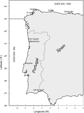
Main landing ports of anglerfish in Portugal and Spain, and the ICES Divisions in the Iberian Atlantic waters.
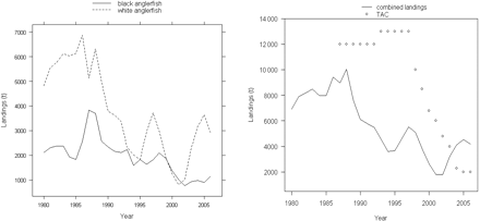
Landings by species (left) and for combined species and annual TAC (right), 1980–2006.
Both stocks are assessed by ICES (International Council for the Exploration of the Sea), as stock units distributed in ICES Divisions VIIIc and IXa (Figure 1). Concerns about the state of the stocks led ICES to advise, from 2000 to 2003, large reductions in fishing mortality and, since 2004, no fishing or the implementation of a recovery plan (ICES, 2007b). The two species have been managed under a common total allowable catch (TAC) since 1987. The TAC was set at very high levels until 1999, between 10 000 and 13 000 t, not restricting the fishery at all (Figure 2). Since 2005, despite the ICES advice, the TAC has been 2000 t.
The Iberian anglerfish stocks have been assessed formally by ICES since 1990 and, using biomass dynamic models, since 1998. Only very small quantities of anglerfish are caught in bottom trawl surveys carried out by Spain and Portugal, so these indices are not considered to reflect the abundance of the two species. Therefore, stock parameters and trajectories in relation to reference points are estimated by fitting a biomass dynamic model, as implemented by Prager (2004), to dataseries of landings and commercial catch per unit effort (cpue). In 2007, the assessment was carried out by anglerfish species (ICES, 2007a) and this procedure was regarded as an improvement on previous ones because it allowed scientists to track and detect different levels of biomass and exploitation by species. The different biological characteristics of the two species supported such separation in the stock assessment. However, for the assessments, only a part of the available abundance indices was used.
The aim of this study is to investigate, by species, whether common patterns exist in the available time-series of abundance indices and, if so, how the common trends (CTs) relate to known features of the exploited areas and fleets. CTs are extracted using dynamic factor analysis (DFA; Zuur et al., 2003a). Also, for white anglerfish, we used the CTs we found as input to a biomass dynamic model, to investigate whether that approach, novel in stock assessment, would improve model fitting and reduce the uncertainty in the parameter estimates and related quantities. We also contrasted our results with estimates obtained using all time-series of abundance. Finally, we look at the utility of this approach for other model-based assessments.
Material and methods
Data available by species were time-series of total annual landings for the period 1980–2006 and six cpue series from Spanish and Portuguese trawlers and from Spanish gillnetters, which we used as abundance indices. Some of the abundance index series had a shorter time frame: the Spanish gillnetter time-series has become available only since 1999, and both Portuguese trawl abundance indices have been available only since 1989 (Table 1).
| Name . | Main fishing area . | Code . | Time frame . |
|---|---|---|---|
| Spanish Trawl Santander | VIIIc, East Cantabrian Sea | STS | 1986–2006 |
| Spanish Trawl Avilés | VIIIc, West Cantabrian Sea | STA | 1986–2003 |
| Spanish Trawl A Coruña | VIIIc, Galician waters | STC | 1986–2006 |
| Spanish Gillnets Cedeira | VIIIc, Galician waters | SGC | 1999–2006 |
| Portuguese Trawl Crustaceans | IXa, Southwest and South of Portugal | PTC | 1989–2006 |
| Portuguese Trawl Fish | IXa, Portuguese waters | PTF | 1989–2006 |
Dynamic factor analysis
DFA is a multivariate time-series analysis that allows the estimation of underlying CTs in short and non-stationary time-series. It has been applied with success in several areas, e.g. time-series of squid catches (Zuur and Pierce, 2004), and species biodiversity (Sousa et al., 2006). The DFA technique resembles a factor analysis (FA) in the sense that new variables (factors) are created that, although many fewer in number than the original variables, are expected to explain most of the variation. The main feature in DFA is that the new axes (CTs in time-series) are smooth functions (curves) over time, with smoothing estimated automatically as part of a two-step EM (expectation–maximization) algorithm. The conditional expectation of the log-likelihood function is calculated in the first step, then the function is maximized over the entire set of iterations (see detail in Zuur et al., 2003a).

The values of factor loadings and canonical correlations can be used to assess the relationships between variables and the relationships between variables and CTs. The decision on which M to retain, as representing the number of underlying CTs in a time-series, can be made objectively using the Akaike Information Criterion (AIC; Akaike, 1974). As AIC is defined as twice the difference between the log-likelihood function (the measure of fit) and the number of parameters (the penalty), the lowest value of the AIC indicates the best solution.
Here, the DFA technique was applied to the six time-series of abundance by species. Because the units and scale of the abundance indices differ between time-series, these were standardized (mean subtracted and divided by the standard deviation). DFA computations were conducted using the software Brodgar (Highland Statistics Ltd).
Biomass dynamic model


ASPIC was applied to white anglerfish using the time-series of abundance indices and the CTs extracted from the DFA analysis. Uncertainty around model parameter estimates and derived quantities, such as Brely = By/BMSY and Frely = Fy/FMSY, were obtained through residual bootstrapping, with bias correction (Prager, 2004).
Results
Common trends
DFA model-fitting to the six time-series (Figure 3) was carried out, for each species, for a range between one and three CTs. The values of AIC for white anglerfish were 234.9 for one CT, 196.4 for two CTs, and 199.3 for three CTs, so supporting the model with two CTs as the best solution. A solution with two CTs was also retained for black anglerfish, because only a marginal decrease in the value of AIC, from 251.7 to 251.1, was obtained between the fits with two and three CTs. The observed values and the model fit by abundance indices time-series indicated, except the Spanish Trawl Avilés (STA) for black anglerfish, good model fit for both species (Figure 4). An exact fit was obtained for the Portuguese Trawl Fish (PTF). However, additional analysis with model refitting after transforming the time-series (Zuur et al., 2003a) showed that the exact fit of PTF was not attributable to an inappropriate underlying model in either case.
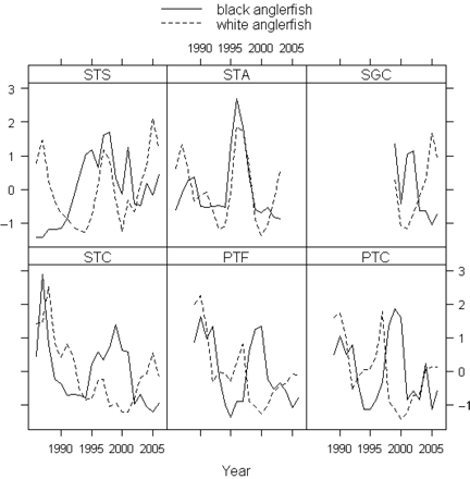
Time-series of abundance indices (standardized) by species. The codes for the time-series are defined in Table 1.
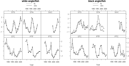
DFA model fit by species, showing observed and fitted abundance indices by time-series. The codes for the time-series are defined in Table 1.
The factor loadings for the DFA model fit with two CTs are presented by species in Figure 5. For white anglerfish, the time-series of the Spanish Gillnets Cedeira (SGC) was clearly related to the first CT, with a factor loading of 0.85. A group joining the abundance indices from the Portuguese Trawl Crustaceans (PTC), the PTF, and the Spanish Trawl A Coruña (STC) was determined by the second CT, but with decreased factor loading magnitude (respectively, 0.70, 0.65, and 0.45), whereas both CTs were important for the Spanish Trawl Santander (STS) and STA series, because those time-series had similar loadings (∼0.5) on both CTs.
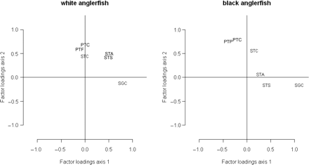
Factor loadings for the DFA model fit with two CTs by species. The codes for the time-series are defined in Table 1.
As for black anglerfish, the SGC was again clearly related to the first CT, with a factor loading of 1.01. Also for the first CT, the STS series contributed, but with less importance (0.41). Both Portuguese trawl indices (PTF and PTC) and the Spanish STC were clearly associated with the second CT, with factor loadings of 0.82 (PTC), 0.80 (PTF), and 0.58 (STC). The abundance index of the STA series made a slight contribution to the first CT, with a factor loading of 0.27, but was not important for the second CT (Figure 5).
The grouping of abundance indices provided by DFA (Figure 5) reflects in part the different areas in which the respective fishing fleets are active. The SGC series is derived mainly from VIIIc-West and is a gillnet fleet exploiting mainly adult anglerfish (total length >50 cm). On the other hand, the other series are trawl fleets exploiting mainly small to medium-sized anglerfish. The STS and STA series are derived mainly from activity in the Cantabrian Sea (VIIIc-East) and PTC, PTF, and STC series mainly from the Atlantic, in the western part of VIIIc (STC) and in IXa (PTC and PTF). Between species, STA and STS series make different contributions to the factor loadings that can partially be explained by the very small proportion of black anglerfish in the landings of those fleets.
The extracted CTs indicate a decrease in abundance of both species from 1980 to the mid-1990s (Figure 6). For the white anglerfish, except a peak in 1997, abundance continued to decrease until 2000, then increased slightly. Both CTs show an increase since 2000, but the first CT indicates a greater relative increase than the second. In contrast to white anglerfish, black anglerfish abundance increased from the mid-1990s to 2000, then decreased, with the first CT indicating a lesser relative decrease.
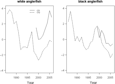
Common trends (y-axes unitless) by species. CT1, first common trend; CT2, second common trend.
Model-fitting and stock parameter estimates
The biomass dynamic model as implemented in ASPIC was fitted to white anglerfish using all six time-series of abundance, hereafter designated by the fit “All”, and the two CTs extracted with the DFA analysis, hereafter designated by the fit “CT”. Model-fitting was carried out using the same initially guessed values in both cases.
The residual values and patterns showed that the model fit “CT” resulted in lower residuals (between −0.16 and 0.16) and an acceptable pattern, particularly for the longer time-series of CT2 (Figure 7). The residual mean square error (RMSE) also indicated a better fit for “CT” (0.11) in relation to the fit “All” (0.53). The proportion of variance explained by the model fit “All” was highest for the STC index (r2 = 0.63), lowest for the STS index (r2 = 0.02), and at intermediate values (r2 = 0.16 to r2 = 0.27) for the STA, SGC, PTF, and PTC indices. For the fit “CT”, results showed best goodness-of-fit for CT2 (0.73) and least for CT1 (0.16), though the latter is a shorter time-series.
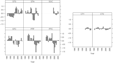
Residual plots (log-scale) by time-series of abundance indices (STS, STA, SGC, STC, PTF, and PTC) and by CTs (CT1 and CT2) for the model fit to white anglerfish.
Estimates of the ratio of initial biomass to K (B1ratio) show similar results for both fits, ∼0.5, indicating that at the beginning of the time-series, the biomass was close to BMSY (Table 2). However, greater relative bias and slightly higher relative interquartile range were obtained for model fit “CT” (Table 2).
Point estimates, relative bias, and relative interquartile ranges for B1ratio, K, r, MSY, and relative biomass in 2007, Brel, and relative fishing mortality in 2006, Frel, obtained by fitting the model with all time-series of abundance indices (All) and with CTs.
| Parameter . | Point estimate . | Relative bias (%) . | Relative IQ range (%) . | |||
|---|---|---|---|---|---|---|
| . | All . | CT . | All . | CT . | All . | CT . |
| B1ratio | 0.54 | 0.46 | 1.3 | 16.8 | 17.2 | 22.6 |
| K (t) | 26 690 | 109 900 | −8.8 | 5.2 | 24.3 | 39.8 |
| r (year−1) | 0.79 | 0.13 | 63.7 | 2.8 | 20.7 | 34.9 |
| MSY (t) | 5 254 | 3 627 | 4.1 | −0.3 | 6.1 | 17.3 |
| Brel 2007 | 0.39 | 0.36 | 34.6 | 11.7 | 359.2 | 27.5 |
| Frel 2006 | 1.48 | 2.18 | 88.3 | −0.9 | 100.8 | 18.7 |
Estimates of K and r were quite different between fits. With the fit “All” the point estimates of (K, r) were (26 690 t, 0.79 year−1), whereas with the fit “CT” they were (109 900 t, 0.13 year−1). Also, the bias has opposite signs for K and there is less relative bias for the fit “CT”, mainly for the parameter r, though dispersion is slightly greater (Table 2). MSY was closer between fits, 5254 t with the fit “All” and 3627 t with the fit “CT”, the latter having less relative bias, but with greater relative interquartile range (Table 2).
Biomass and fishing mortality trajectories
Trends in relative biomass and fishing mortality were similar for both fits (Figure 8). They both estimated a general decrease in biomass over the period 1980–2006, but steeper in the 1980s for the fit “All”. In terms of the trajectory of fishing mortality, both fits estimated an increase in the 1980s and fluctuations thereafter. However, given the low contrast in the biomass trajectories, the trends in relative fishing mortality mimic those in the landings (Figure 2). Also, the 80% confidence intervals (CIs) for fit “CT” are relatively narrow for the whole time-series, whereas the upper bound on relative biomass and, hence, the lower bound for the relative fishing mortality are wide for recent years for the fit “All”, reflecting the high value of bias (Figure 8).
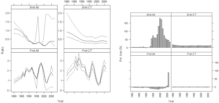
White anglerfish relative biomass and fishing mortality trajectories with 80% bias-corrected CI (left) and relative bias (right), for the period 1980–2006.
The relative biomass and fishing mortality in the final year are indicative of stock status and used to provide management advice. It is therefore important to note that estimates are consistent between fits, both indicating, for 2007, a biomass around 40% below BMSY and a fishing mortality in 2006 above FMSY (Table 2). However, the estimates from fit “All” are highly biased and uncertain.
Discussion
The Iberian anglerfish stocks are assessed by ICES based on commercial cpue series. Abundance indices from research surveys are not reliable because of the poor survey catchability of anglerfish. As for other stocks, there are a number of commercial cpue series available that may show slightly diverging or even contradicting signals for certain periods, which can either be the result of noise or reflect different signals from differing areas or population components. Using all time-series in stock assessment models to provide estimates of population abundance and fishing mortality can result in model inconsistency and may even lead to violation of model assumptions. Using only a few series is often the common practice in stock assessment but this procedure is, often, based on arbitrary and subjective selection of fleets. Our study has shown that the use of DFA to extract CTs from all available series may be a better option than to exclude some time-series subjectively. DFA allows a straightforward analysis of time-series and an interpretation of its discrepancies, also providing new series that enclose the essential signals of the original data. It may be argued that FA could have been used instead. In FA, however, the factors are not exact linear combinations of the original variables: the variables are defined as a linear function of factors apart from an error term. Therefore, to extract CTs from the abundance time-series with FA, it would require reversing that relationship and, according to Jolliffe (2002), this procedure certainly would not lead to an exact relationship between factors and variables. Moreover, analysis with FA and similar techniques does not take into account the time structure of the variables, so similar results will be obtained if the order of time is changed (Zuur et al., 2003b).
The DFA extracted two CTs from the six cpue time-series available for both white and black anglerfish stocks. For both stocks, CTs diverged in the relative level of decrease (black anglerfish) or increase (white anglerfish) since 2000. The cpue series were grouped by the factor loadings, reflecting the exploited area (Atlantic vs. Cantabrian Sea), and exploited population components (mostly juveniles vs. adults). The grouping was coherent and the resulting trends probably reflect the most important signal of the population dynamics.
It was our aim to investigate the effects, through parameter estimates and uncertainty, of using abundance CTs in model-based assessment. We believe that we have shown that the biomass dynamic model fits, with all cpue series and with the abundance CTs carried out for white anglerfish, yielded different results and, in particular, different model goodness-of-fit. For the most important stock status diagnostic, i.e. the relative biomass and relative fishing mortality of the final year in the time-series, the fit with all cpue series showed high bias and high uncertainty. With that fit, stock status should be considered unknown, because the 80% CI of relative biomass included values below and above 1, and the same for relative fishing mortality. Also, the r parameter was estimated to be high, >0.5 year−1, contradicting the available biological information that considers anglerfish as long-lived species. According to Punt and Hilborn (1996), the r parameter should be in the range 0.1–0.4 year−1 for long-lived species.
On the other hand, the model fit with the CTs as abundance indices showed low bias and acceptable CIs. The results gave a probability >80% of biomass being below BMSY and fishing mortality being above FMSY. The r parameter, estimated to be 0.13 year−1, is also more in agreement with the available biological information, showing acceptable bias and CIs.
The MSY was estimated to be 5200 t with the fit “All”. This value seems high, because landings only exceeded 5200 t in a few years at the beginning of the period (Figure 2), but the stock apparently could not sustain such large catches and the relative biomass decreased thereafter. With the fit “CT” the estimated MSY was lower, at 3600 t, more consistent with the stock trajectory and landings, because landings >3600 t have been observed for a longer period and stock recoveries in the late 1990s and early 2000s again brought landings up to that level.
The relative biomass shows similar trends throughout the time-series between both model fits, with biomass decreasing from the beginning of the time-series until the mid-1990s. Thereafter, small recoveries are apparent in the late 1990s and early 2000s. However, the white anglerfish biomass recovery is different between fits. The fit “All” estimated a higher r and MSY, a lower K, and steeper biomass recoveries, but results from that fit showed very high bias and uncertainty, in particular for the biomass estimates (Figure 8). Associated with the low r parameter for the fit “CT”, biomass changes were more restricted, and the estimates of relative fishing mortality tended to follow the landings more closely.
Comparing our results with those from the stock assessment carried out by ICES (2007a), which used the same biomass dynamic model but with only the cpue series of STC and SGC, our results for the fit “All” are similar to those of ICES for the estimated MSY, K, and r parameters (the B1ratio cannot be directly compared because the time-series is different). However, the relative biomass and fishing mortality of the final year estimated by ICES, which has acceptable bias and 80% CIs, are similar to our estimates with the fit “CT”.
We have provided a provisional first set of results on applying DFA for stock assessment purposes using a biomass dynamic model. Lower estimates of bias and narrower CIs were obtained for relative biomass and relative fishing mortality, but to assess and quantify the effect of the approach in the estimates of variance of the model parameters and possible bias, we need to carry out and evaluate a simulation exercise.
Here, we applied DFA to cpue data, but the technique can be used also for survey data. This may be particularly useful when the purpose is to combine stock survey data available from different countries in adjacent areas, and can perhaps be an alternative to current approaches (e.g. southern horse mackerel; ICES, 2007c). The approach presented here can be extended easily to age-based models. The abundance CTs, from cpue and/or survey data, can be used as relative biomass indices in the virtual population analysis (VPA) tuning process by adding an extra term to the model's objective function, for example in a similar manner to how it is implemented currently in integrated catch-at-age analysis (Patterson and Melvin, 1996) or ADAPT (Gavaris, 1988). Further research is, however, required to investigate whether parameter estimates and uncertainty are improved by using annual abundance CTs for VPA tuning. Another challenging task would be to develop the approach presented here to take account of the age structure of the stock, which indices by age can provide.
Acknowledgements
We thank the EU project ABA “Improving the quality of Southern Anglerfish stocks assessment” (FISH/2004/03-22), for co-financing this work.


