


Abstract
Is there risk of selection bias in etiological studies investigating prenatal risk factors of poor male fecundity in a cohort of young men?
The risk of selection bias is considered limited despite a low participation rate.
Participation rates in studies relying on volunteers to provide a semen sample are often very low. Many risk factors for poor male fecundity are associated with participation status, and as men with low fecundity may be more inclined to participate in studies of semen quality, a risk of selection bias exists.
A population-based follow-up study of 5697 young men invited to the Fetal Programming of Semen Quality (FEPOS) cohort nested within the Danish National Birth Cohort (DNBC), 1998–2019.
Young men (age range: 18 years, 9 months to 21 years, 4 months) born 1998–2000 by mothers included in the DNBC were invited to participate in FEPOS. In total, 1173 men answered a survey in FEPOS (n = 115 participated partly); of those, 1058 men participated fully by also providing a semen and a blood sample at a clinical visit. Differential selection according to parental baseline characteristics in the first trimester, the sons’ own characteristics from the FEPOS survey, and urogenital malformations and diseases in reproductive organs from the Danish registers were investigated using logistic regression. The influence of inverse probability of selection weights (IPSWs) to investigate potential selection bias was examined using a predefined exposure-outcome association of maternal smoking in the first trimester (yes, no) and total sperm count analysed using adjusted negative binomial regression. A multidimensional bias analysis on the same association was performed using a variety of bias parameters to assess different scenarios of differential selection.
Participation differed according to most parental characteristics in first trimester but did not differ according to the prevalence of a urogenital malformation or disease in the reproductive organs. Associations between maternal smoking in the first trimester and male fecundity were similar when the regression models were fitted without and with IPSWs. Adjusting for other potential risk factors for poor male fecundity, maternal smoking was associated with 21% (95% CI: −32% to −9%) lower total sperm count. In the bias analysis, this estimate changed only slightly under realistic scenarios. This may be extrapolated to other exposure-outcome associations.
We were unable to directly assess markers of male fecundity for non-participants from, for example an external source and therefore relied on potential proxies of fecundity. We did not have sufficient power to analyse associations between prenatal exposures and urogenital malformations.
The results are reassuring when using this cohort to identify causes of poor male fecundity. The results may be generalized to other similar cohorts. As the young men grow older, they can be followed in the Danish registers, as an external source, to examine, whether participation is associated with the risk of having an infertility diagnosis.
The project was funded by the Lundbeck Foundation (R170-2014-855), the Capital Region of Denmark, Medical doctor Sofus Carl Emil Friis and spouse Olga Doris Friis’s Grant, Axel Muusfeldt’s Foundation (2016-491), AP Møller Foundation (16-37), the Health Foundation, Dagmar Marshall’s Fond, Aarhus University and Independent Research Fund Denmark (9039-00128B). The authors declare that they have no conflict of interest.
N/A.
Introduction
Suboptimal sperm count is prevalent (Skakkebaek et al., 2016; Levine et al., 2017; Keglberg Hærvig et al., 2020), and is associated with low fecundity and longer time to pregnancy (Bonde et al., 1998). This may increase the use of assisted reproductive technologies, which is rising in Europe (Ferraretti et al., 2017). Therefore, it is of key interest to identify modifiable causes of compromised male fecundity (Skakkebaek et al., 2016; Keglberg Hærvig et al., 2020).
Participation rates in studies examining semen quality are often very low (<20%) (Handelsman, 1997; Andersen et al., 2000; Cohn et al., 2002; Eustache et al., 2004; Muller et al., 2004; Stewart et al., 2009; Keglberg Hærvig et al., 2020), and potential selection bias in these studies is therefore of great concern (Handelsman, 1997; Levine et al., 2017). Men agreeing to participate may represent a subfecund population that chooses to participate due to concern about their potential to father a child (Handelsman, 1997), for example due to couple infertility or due to knowledge about parents’ fecundity. If participation is also associated with the exposure of interest (Fig. 1A), selection bias may be introduced due to differential participation of study participants (Hernan et al., 2004).

Directed acyclic graphs (DAGs) illustrating different causal frameworks for the potential sources of selection bias in the fetal programming of semen quality (FEPOS) cohort, Denmark, 1998–2019. U represents potential unknown factors, E represents a given exposure under study and boxes indicate conditioning. (A) DAG illustrating the potential selection bias in FEPOS. (B) DAG illustrating the causal framework for the use of information on urogenital malformations or diseases in reproductive organs as proxies in evaluating the potential sources of selection bias in FEPOS. Urogenital malformation or reproductive diseases may cause low semen quality and poor fecundity, and may affect the motivation to participate in FEPOS. (C) DAG illustrating that urogenital malformations or diseases in reproductive organs were not associated with participation. (D) DAG illustrating the potential source of selection bias due to the advice to decline participation, if the young men did not have both testes. Conditioning on the young men not having cryptorchidism (cryptorchidism = 0) may partly remove some of the total effect of an exposure on male fecundity, and may also introduce potential selection bias through U2 or M-bias through U1 and U2. (E) DAG illustrating the best case scenario in evaluating the potential sources of selection bias in FEPOS. Neither the proxies (parental couple fecundity and urogenital malformations or diseases in the reproductive organs) nor male fecundity was likely associated with participation in FEPOS.
Though some previous studies investigating potential selection bias in studies of semen quality and male fecundity are reassuring with regards to selection bias (Cohn et al., 2002; Eustache et al., 2004; Muller et al., 2004; Hauser et al., 2005; Ramlau-Hansen et al., 2007; Stewart et al., 2009), it remains to be elucidated whether selection bias in a population-based sample of young men, likely to be unaware of their reproductive potential, may threaten the validity of study results. Moreover, the use of inverse probability of selection weights (IPSWs) to adjust for potential selection bias in studies of semen quality or male fecundity remains to be examined. In addition, no studies have performed bias analyses to assess the magnitude of potential selection bias in these studies. Therefore, we aimed to investigate the nature of participation, evaluate the influence of applying IPSWs and to perform a multidimensional bias analysis to assess the risk of selection bias in a newly established population-based male-offspring cohort.
Materials and methods
Study population
The Fetal Programming of Semen Quality (FEPOS) cohort (Keglberg Hærvig et al., 2020), nested within the Danish National Birth Cohort (DNBC) (Olsen et al., 2001), was established with the aim of identifying potential modifiable foetal exposures associated with poor semen quality, low testes volume and altered reproductive hormone levels in young adult men (Haervig et al., 2020; Gaml-Sørensen et al., 2022; Hærvig et al., 2022; Ugelvig Petersen et al., 2022). The data collection in FEPOS included a comprehensive online questionnaire on health and health behaviour in addition to a clinical visit, where the participants were invited to provide a semen, urine and a blood sample in addition to self-measuring their testes volume.
For the young adult sons to be invited to this male-offspring cohort, the mothers had to be enrolled in the DNBC, they should have completed two computer-assisted telephone interviews in pregnancy (approx. gestational weeks 16 and 31) in addition to having provided a gestational blood sample for storage in the Danish National Biobank. The sons should be at least 18 years and 9 months at the time of invitation and live near Copenhagen or Aarhus, where the clinical visits were to take place.
Enrolment to the FEPOS cohort began in March 2017 by use of a comprehensive recruitment system using ‘e-boks’, which is a secure digital mailbox that all Danish citizens have access to and use in communication with authorities. In total, 21 623 young men were eligible for participation, and of those, 5697 received an invitation letter. There were no exclusion criteria per se, however, the sons were advised to decline participation, if they lacked one or both testes, had vasectomy or chemotherapy (Keglberg Hærvig et al., 2020). When inclusion ended in December 2019, 1173 young men had completed the FEPOS survey (n = 115 participating partly), and of these 1058 also participated in the clinical visit (participating fully) (Fig. 2). The participants who participated in the clinical visit received a compensation of 500 DKK (≈67 Euro).
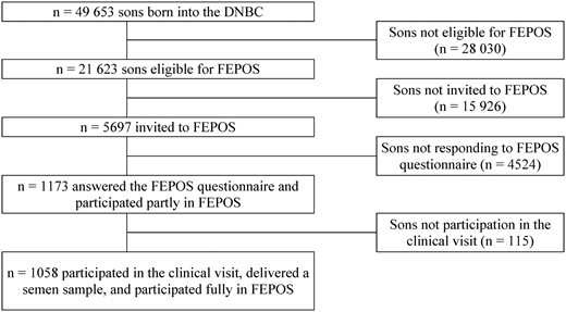
Flowchart of the inclusion of participants in the fetal programming of semen quality (FEPOS) cohort, nested within the Danish National Birth Cohort (DNBC), Denmark, 1998–2019.
Data sources
Comprehensive baseline information from the DNBC was available for all those invited to FEPOS. Many baseline lifestyle and socioeconomic factors possibly affect the young men’s inclination to participate in cohort studies, and the following variables from the first DNBC interview were included to consider whether participants and non-participants differed in terms of baseline characteristics: socioeconomic status of the parents, cohabitation of the parents, maternal smoking (Brix et al., 2018), maternal alcohol intake (Brix et al., 2020), maternal pre-pregnancy BMI and paternal smoking. Specifically, as a proxy for male fecundity or potential awareness of fecundity potential, we investigated whether parental couple fecundity was associated with participation. From the Danish Medical Birth Register, we included maternal age at delivery, birth weight and gestational age. These variables are described in further detail in Supplementary Data File S1.
We had information on the young men’s own health behavioural factors for those participating fully or partly. The following variables from the FEPOS survey were included to investigate whether those participating partly differed from those participating fully: occupation, smoking, alcohol intake, unhealthy diet, pubertal timing, sexual experience and knowledge of own fertility. These variables are also described in Supplementary Data File S1.
We had no information on markers of male fecundity from the non-participants, and no external data source could provide this information. However, The Danish National Patient Register (DNPR) holds complete information on diagnostic codes (ICD10) from all hospital contacts 1995 and onwards (Schmidt et al., 2015). We investigated the following variables as proxies for male fecundity for participants and non-participants (Fig. 1B): cryptorchidism, hypospadias or any urogenital malformation; hydrocele, torsio testis, orchitis or any disease in the reproductive organs. All malformations and diseases were identified from the date of birth until the date of completing the FEPOS questionnaire for each son. The codes used to derive these variables are listed in Supplementary Data File S1.
Statistical analyses
Potential differential participation according to parental characteristics, the son’s own characteristics and diagnoses derived from the DNPR were described by means (with standard deviations) and frequencies and examined using logistic regression models. The logistic regression models were chosen to ensure that model-based probabilities of selection were bound between 0 and 1, and to mimic bias parameters used for internal adjustment in FEPOS studies, but also to provide other researchers with bias parameters for selection bias adjustment as proposed by Thompson and Arah (2014). Unadjusted and adjusted odds ratios (ORa) of participation in FEPOS with 95% CI were estimated for all available data: the parental baseline characteristics (Table I), the young men’s own health behavioural factors (Table II), and for diagnoses of urogenital malformations and diseases in reproductive organs (Table III). Hence, relative to the chosen reference values for each variable, an ORa>1 indicated a higher probability of participation and an ORa<1 indicated a lower probability of participation.
Participation status according to parental baseline characteristics and unadjusted and adjusted odds ratios for participation for 5697 invited young men from the fetal programming of semen quality (FEPOS) cohort, Denmark, 1998–2019.
| Participation | Odds ratiosa | |||||||||
|---|---|---|---|---|---|---|---|---|---|---|
| Non-participants | Participants | Unadjusted (CI 95%) | Adjustedb (CI 95%) | Missings | ||||||
| No. | % | No. | % | No. | % | |||||
| 4639 | 81 | 1058 | 19 | |||||||
| Maternal alcohol (drinks/week)c | 0.6 (1.0) | 0.7 (1.1) | >12d | >0.2 | ||||||
| 0 | 2626 | 57 | <556d | <53 | Ref. | Ref. | ||||
| 0.1–1.0 | 1311 | 28 | 330 | 31 | 1.19 | (1.02–1.39) | 1.21 | (1.03–1.41) | ||
| 1.1–3.0 | 570 | 12 | 140 | 13 | 1.16 | (0.95–1.43) | 1.20 | (0.97–1.48) | ||
| >3.0 | 120 | 3 | 32 | 3 | 1.26 | (0.85–1.88) | 1.36 | (0.90–2.05) | ||
| Couple fecundity (TTP+MAR) | 19 | 0.3 | ||||||||
| Unplanned pregnancy | 699 | 15 | 175 | 17 | 0.93 | (0.75–1.15) | 0.92 | (0.73–1.15) | ||
| 0 months | 993 | 21 | 268 | 25 | Ref. | Ref. | ||||
| 1–2 months | 937 | 20 | 209 | 20 | 0.83 | (0.68–1.01) | 0.83 | (0.67–1.02) | ||
| 3–5 months | 827 | 18 | 155 | 15 | 0.69 | (0.56–0.86) | 0.72 | (0.57–0.90) | ||
| 6–12 months | 540 | 12 | 107 | 10 | 0.73 | (0.57–0.94) | 0.75 | (0.58–0.96) | ||
| >12 months | 350 | 8 | 72 | 7 | 0.76 | (0.57–1.02) | 0.80 | (0.59–1.07) | ||
| MAR | 280 | 6 | 66 | 6 | 0.87 | (0.65–1.18) | 0.93 | (0.68–1.27) | ||
| Maternal age at delivery (years)c | 31 (4) | 31 (4) | <5d | 0 | ||||||
| –24.9 | 324 | 7 | 69 | 7 | Ref. | Ref. | ||||
| 25–29.9 | 1676 | 36 | 374 | 35 | 1.05 | (0.79–1.39) | 0.96 | (0.71–1.31) | ||
| 30–34.9 | 1843 | 40 | <430d | <41 | 1.09 | (0.83–1.45) | 0.95 | (0.70–1.29) | ||
| 35– | 796 | 17 | 185 | 17 | 1.09 | (0.80–1.48) | 0.93 | (0.66–1.30) | ||
| Maternal BMI (kg/m2)c | 22.9 (3.8) | 22.8 (3.6) | 117 | 2 | ||||||
| <18.5 | 233 | 5 | 64 | 6 | 1.22 | (0.91–1.62) | 1.19 | (0.88–1.59) | ||
| 18.5 to <24.9 | 3353 | 72 | 758 | 72 | Ref. | Ref. | ||||
| 25 to <29.9 | 728 | 16 | 164 | 16 | 1.00 | (0.83–1.20) | 1.06 | (0.87–1.28) | ||
| >30 | 233 | 5 | 47 | 4 | 0.89 | (0.65–1.23) | 1.00 | (0.71–1.39) | ||
| Parental highest social class | 0 | 0 | ||||||||
| High-grade professional | 1426 | 31 | 359 | 34 | Ref. | Ref. | ||||
| Low-grade professional | 1396 | 30 | 350 | 33 | 1.00 | (0.84–1.17) | 1.05 | (0.88–1.24) | ||
| Skilled worker | 1106 | 24 | 202 | 19 | 0.73 | (0.60–0.88) | 0.78 | (0.64–0.96) | ||
| Unskilled worker | 568 | 12 | 98 | 9 | 0.69 | (0.54–0.87) | 0.69 | (0.53–0.90) | ||
| Student/Economically inactive | 143 | 3 | 49 | 5 | 1.36 | (0.96–1.92) | 1.42 | (0.98–2.06) | ||
| Parental cohabitation | <5d | 0 | ||||||||
| Yes | <4564d | <98 | 1036 | 98 | Ref. | Ref. | ||||
| No | 75 | 2 | 22 | 2 | 1.29 | (0.80–2.09) | 1.28 | (0.75–2.17) | ||
| Paternal smoking | 5 | 0 | ||||||||
| No | <3229d | <70 | <751d | <71 | Ref. | Ref. | ||||
| Yes | 1410 | 30 | 307 | 29 | 0.94 | (0.81–1.08) | 1.04 | (0.89–1.22) | ||
| Maternal smoking (cigarettes/day)c | 1.8 (3.9) | 1.4 (3.7) | 19 | 0.3 | ||||||
| 0 | 3384 | 73 | 815 | 77 | Ref. | Ref. | ||||
| 1–10 | 1037 | 22 | 205 | 19 | 0.82 | (0.69–0.97) | 0.85 | (0.71–1.01) | ||
| >10 | 199 | 4 | 38 | 4 | 0.79 | (0.56–1.13) | 0.80 | (0.54–1.18) | ||
| Gestational age (weeks)c | 40 + 0 (1.6) | 40 + 0 (1.6) | >28d | 0.6 | ||||||
| ≥37 + 0 | 4424 | 95 | <1013d | <96 | Ref. | Ref. | ||||
| <37 + 0 | 187 | 4 | 45 | 4 | 1.06 | (0.76–1.47) | 1.34 | (0.90–1.99) | ||
| Birth weight (g)c | 3638 (549) | 3701 (549) | 71 | 1 | ||||||
| ≥2500 | 4464 | 96 | 1025 | 97 | Ref. | Ref. | ||||
| <2500 | 120 | 3 | 17 | 2 | 0.62 | (0.37–1.03) | 0.44 | (0.24–0.82) | ||
Information on all baseline characteristics were collected in first trimester with the exception of information on maternal age at delivery, birth weight and gestational age, which was obtained at birth. The percentages may not add up to 100% due to rounding to the nearest number.
TTP, time to pregnancy; MAR, medically assisted reproduction; OR, odds ratio; Ref., reference category.
An OR >1 indicate higher odds of participation and an OR <1 indicate lower odds of participation relatively to the reference category.
Adjusted for the other baseline characteristics from the table with the exception of birth weight and gestational age at delivery, which is considered to be factors influenced by the other baseline characteristics and not influencing the other baseline characteristics.
Continuous variables also presented as mean (SD).
Due to local data regulations it is not allowed to report smaller numbers than five, why the numbers in the table have been changed to mask the numbers smaller than five.
Participation status according to parental and own baseline characteristics and unadjusted and adjusted odds ratios for participation for 1173 young men answering the pre-clinical survey from the fetal programming of semen quality (FEPOS) cohort, Denmark, 1998–2019.
| Participation | Odds ratiosa | |||||||||
|---|---|---|---|---|---|---|---|---|---|---|
| Participating partly | Participating fully | Unadjusted (CI 95%) | Adjustedb (CI 95%) | Missings | ||||||
| No. | % | No. | % | No. | % | |||||
| 115 | 10% | 1058 | 90% | |||||||
| Parental characteristics | ||||||||||
| Maternal alcohol (drinks/week)c | 0.7 (1.0) | 0.7 (1.1) | <5d | <0.4 | ||||||
| 0 | 61 | 53 | <556d | <53 | Ref. | Ref. | ||||
| 0.1–1.0 | 35 | 30 | 330 | 31 | 1.04 | (0.67–1.60) | 1.06 | (0.67–1.70) | ||
| 1.1–3.0 | >14d | >12 | 140 | 13 | 0.96 | (0.54–1.72) | 0.91 | (0.50–1.67) | ||
| >3.0 | <5d | <5 | 32 | 3 | 1.17 | (0.35–3.94) | 1.27 | (0.36–4.43) | ||
| Couple fecundity (TTP+MAR) | <11d | <1 | ||||||||
| Unplanned pregnancy | 11 | 10 | 175 | 17 | 1.72 | (0.84–3.54) | 1.91 | (0.89–4.09) | ||
| 0 months | <30d | <26 | 268 | 25 | Ref. | Ref. | ||||
| 1–2 months | 22 | 19 | 209 | 20 | 1.03 | (0.57–1.84) | 1.13 | (0.62–2.07) | ||
| 3–5 months | 18 | 16 | 155 | 15 | 0.93 | (0.50–1.73) | 0.97 | (0.52–1.81) | ||
| 6–12 months | 18 | 16 | 107 | 10 | 0.64 | (0.34–1.21) | 0.70 | (0.37–1.35) | ||
| >12 months | 7 | 6 | 72 | 7 | 1.11 | (0.47–2.64) | 1.09 | (0.45–2.64) | ||
| MAR | 9 | 8 | 66 | 6 | 0.79 | (0.36–1.76) | 0.80 | (0.36–1.81) | ||
| Maternal age at deliveryc | 31.5 (4) | 31 (4) | <5d | <0.4 | ||||||
| –24.9 | 10 | 9 | 69 | 7 | Ref. | Ref. | ||||
| 25–29.9 | 35 | 30 | 374 | 35 | 1.55 | (0.73–3.27) | 1.87 | (0.85–4.12) | ||
| 30–34.9 | 47 | 41 | <430d | <41 | 1.32 | (0.64–2.74) | 1.77 | (0.80–3.95) | ||
| 35– | 23 | 20 | 185 | 17 | 1.17 | (0.53–2.57) | 1.59 | (0.66–3.81) | ||
| Maternal BMI (kg/m2)c | 22.4 (3.1) | 22.8 (3.6) | 28 | 2 | ||||||
| <18.5 | <5d | <5 | 64 | 6 | 2.39 | (0.74–7.78) | 2.38 | (0.72–7.84) | ||
| 18.5 to <24.9 | 85 | 74 | 758 | 72 | Ref. | Ref. | ||||
| 25 to <29.9 | 23 | 20 | 164 | 16 | 0.80 | (0.49–1.31) | 0.85 | (0.51–1.39) | ||
| >30 | <5d | <5 | 47 | 4 | 5.27 | (0.72–38.69) | 5.60 | (0.75–41.63) | ||
| Parental highest social class | 0 | 0 | ||||||||
| High-grade professional | >44d | >38 | 359 | 34 | Ref. | Ref. | ||||
| Low-grade professional | 34 | 30 | 350 | 33 | 1.35 | (0.85–2.15) | 1.41 | (0.86–2.30) | ||
| Skilled worker | 21 | 18 | 202 | 19 | 1.26 | (0.73–2.17) | 1.25 | (0.70–2.23) | ||
| Unskilled worker | 11 | 10 | 98 | 9 | 1.17 | (0.58–2.33) | 1.11 | (0.51–2.40) | ||
| Student/Economically inactive | <5d | <5 | 49 | 5 | 3.21 | (0.76–13.62) | 3.58 | (0.77–16.62) | ||
| Parental cohabitation | 0 | 0 | ||||||||
| Yes | >110d | >95 | 1036 | 98 | Ref. | Ref. | ||||
| No | <5d | <5 | 22 | 2 | 0.79 | (0.23–2.69) | 0.36 | (0.09–1.48) | ||
| Paternal smoking | <5d | <0.4 | ||||||||
| No | 82 | 71 | <751d | <71 | Ref. | Ref. | ||||
| Yes | 33 | 29 | 307 | 29 | 1.02 | (0.66–1.56) | 0.94 | (0.59–1.51) | ||
| Maternal smoking (cigarettes/day)c | 1.4 (3.8) | 1.4 (3.7) | 0 | 0 | ||||||
| 0 | 90 | 78 | 815 | 77 | Ref. | Ref. | ||||
| 1–10 | >20d | >17 | 205 | 19 | 1.08 | (0.65–1.78) | 1.10 | (0.63–1.90) | ||
| >10 | <5d | <5 | 38 | 4 | 1.05 | (0.37–3.01) | 0.90 | (0.29–2.80) | ||
| Gestational age (weeks)c | 40 + 0 (1.4) | 40 + 0 (1.6) | <5d | <0.4 | ||||||
| ≥37 + 0 | >110d | >95 | <1013d | <96 | Ref. | Ref. | ||||
| <37 + 0 | <5d | <5 | 45 | 4 | 2.52 | (0.60–10.53) | 2.54 | (0.59–10.85) | ||
| Birth weight (g)c | 3636 (580) | 3701 (549) | >16d | 2 | ||||||
| ≥2500 | >110d | >95 | 1025 | 97 | Ref. | Ref. | ||||
| <2500 | <5d | <5 | 17 | 2 | 0.44 | (0.15–1.34) | 0.38 | (0.12–1.25) | ||
| Sons own characteristics | ||||||||||
| Occupation | <5d | <0.4 | ||||||||
| High school | <59d | <51 | <575d | <55 | Ref. | Ref. | ||||
| Other education | 17 | 15 | 201 | 19 | 1.20 | (0.68–2.11) | 0.79 | (0.38–1.65) | ||
| Sabbatical year | 19 | 17 | 153 | 14 | 0.82 | (0.47–1.41) | 0.54 | (0.26–1.13) | ||
| Other | 20 | 17 | 129 | 12 | 0.65 | (0.38–1.13) | 0.90 | (0.39–2.04) | ||
| Unhealthy diet | 7 | 0.6 | ||||||||
| ≤2 days/week | <86d | <75 | <770d | <73 | Ref. | Ref. | ||||
| ≥3 days/week | 29 | 25 | 288 | 27 | 1.06 | (0.68–1.66) | 1.22 | (0.62–2.37) | ||
| Smoking | <11d | <1 | ||||||||
| No, never | 56 | 49 | <510d | <48 | Ref. | Ref. | ||||
| No, former | 14 | 12 | 135 | 13 | 1.33 | (0.68–2.60) | 1.25 | (0.53–2.93) | ||
| Yes, occasionally | 28 | 24 | 281 | 27 | 1.11 | (0.69–1.79) | 1.32 | (0.66–2.66) | ||
| Yes, every day | 11 | 10 | 132 | 12 | 1.07 | (0.58–1.97) | 0.90 | (0.38–2.16) | ||
| Alcohol intake | <11d | <1 | ||||||||
| <1/month | 17 | 15 | 117 | 11 | Ref. | Ref. | ||||
| 1–3 times/month | 36 | 31 | <376d | <36 | 1.51 | (0.82–2.78) | 2.38 | (0.97–5.85) | ||
| 1/week | 28 | 24 | 268 | 25 | 1.39 | (0.73–2.64) | 1.46 | (0.61–3.48) | ||
| ≥2/week | 28 | 24 | 297 | 28 | 1.54 | (0.81–2.92) | 1.91 | (0.80–4.57) | ||
| Puberty | 236 | 20 | ||||||||
| Earlier than peers | 14 | 12 | 180 | 17 | 1.59 | (0.87–2.89) | 1.34 | (0.65–2.73) | ||
| Same time as peers | 70 | 61 | 567 | 54 | Ref. | Ref. | ||||
| Later than peers | 9 | 8 | 97 | 9 | 1.33 | (0.64–2.75) | 1.12 | (0.47–2.69) | ||
| Sexual experiencee | <12d | <1 | ||||||||
| No | 21 | 18 | 164 | 16 | Ref. | Ref. | ||||
| Yes | 87 | 76 | <894d | <84 | 1.31 | (0.79–2.17) | 1.13 | (0.62–2.04) | ||
| Known fertilitye | 503 | 43 | ||||||||
| No | 60 | 52 | 580 | 55 | Ref. | |||||
| Yes | 7 | 6 | 24 | 2 | 0.35 | (0.15–0.86) | 0.33 | (0.12–0.90) | ||
The percentages may not add up to 100% due to rounding to the nearest number. Information on all baseline characteristics were collected in first trimester with the exception of information on maternal age at delivery, birth weight and gestational age, which was obtained at birth. Information on all sons’ own characteristics were collected from the pre-clinical survey in FEPOS.
TTP, time to pregnancy; MAR, medically assisted reproduction; Ref., reference category; OR, odds ratio.
An OR >1 indicate higher odds of participation and an OR<1 indicate lower odds of participation relatively to the reference category.
Parental characteristics adjusted for the other baseline characteristics from the table with the exception of birth weight and gestational age at delivery, which is considered to be factors influenced by the other baseline characteristics and not influencing the other baseline characteristics. Sons own characteristics adjusted for the remaining sons’ baseline characteristics.
Continuous variables also presented as mean (SD).
Due to local data regulations it is not allowed to report smaller numbers than five, why the numbers in the table have been changed to mask the numbers smaller than five.
Sexual experience not adjusted for known fertility and known fertility not adjusted for sexual experience.
Participation status according to urogenital malformations and diseases and unadjusted and adjusted odds ratios for participation in 5697 invited young men from the fetal programming of semen quality (FEPOS) cohort, Denmark, 1998–2019.
| Participation | Odds ratiosa | |||||||
|---|---|---|---|---|---|---|---|---|
| Non-participants | Participants | Unadjusted (CI 95%) | Adjustedb (CI 95%) | |||||
| No. | % | No. | % | |||||
| 4639 | 81 | 1058 | 19 | |||||
| Any urogenital malformation | ||||||||
| No | 4482 | 97 | 1024 | 97 | Ref. | Ref. | ||
| Yes | 157 | 3 | 34 | 3 | 0.95 | (0.65–1.38) | 0.93 | (0.63–1.37) |
| Cryptorchidism | 124 | 2.7 | 26 | 2.5 | 0.92 | (0.60–1.41) | 0.89 | (0.57–1.39) |
| Hypospadia | 29 | 0.6 | 7 | 0.7 | 1.06 | (0.46–2.42) | 0.91 | (0.37–2.21) |
| Any disease in reproductive organs | ||||||||
| No | 4200 | 91 | 963 | 91 | Ref. | Ref. | ||
| Yes | 439 | 9 | 95 | 9 | 0.94 | (0.75–1.19) | 0.96 | (0.76–1.21) |
| Hydrocele | 63 | 1.4 | 10 | 1.0 | 0.69 | (0.35–1.36) | 0.69 | (0.35–1.36) |
| Torsio testis | 56 | 1.2 | 7 | 0.7 | 0.55 | (0.25–1.20) | 0.57 | (0.26–1.26) |
| Orchitis | 43 | 0.9 | 7 | 0.7 | 0.71 | (0.32–1.59) | 0.73 | (0.33–1.64) |
The percentages may not add up to 100% due to rounding to the nearest number.
Information on urogenital malformations and diseases in reproductive organs were collected from date of birth and until the date of answering the pre-clinical survey in FEPOS.
Ref., reference category; OR, odds ratio.
An OR >1 indicate higher odds of participation and an OR<1 indicate lower odds of participation relatively to the reference category.
Adjusted for highest socioeconomic status of the parents, couple fecundity, cohabitation of the parents, maternal smoking, maternal alcohol intake, maternal pre-pregnancy body mass index, maternal age at delivery and paternal smoking.
Using the baseline characteristics available for all young men invited to FEPOS, IPSWs can be calculated and used for internal adjustment for potential selection bias. This can be done assuming that all explanatory variables associated with participation are included in the calculation, and that there is no residual confounding, indicating that participants may in fact represent non-participants in the exposure—outcome association (Hernan et al., 2004; Thompson and Arah, 2014). The probability of participation was calculated using a multivariable logistic regression model, and the inverse of this probability, the IPSW, was assigned to each participant to reweight the participants into a pseudo-population representative of all young men invited to FEPOS. This pseudo-population represents a population without selection, given that the directed acyclic graph (DAG) for identifying the explanatory variables was correctly specified (Hernan et al., 2004). The IPSWs are further described in Supplementary Data File S2.
To assess the effect of applying the IPSWs, we estimated predefined associations between maternal smoking (yes, no), which is an established risk factor for low fecundity in male offspring (Ramlau-Hansen et al., 2007; Håkonsen et al., 2014; Hærvig et al., 2022). Maternal smoking was associated with participation (Table I) and associated with markers of male fecundity (Table IV). The associations were estimated by use of negative binomial regression models (Stata’s nbreg package), adjusted for the different baseline characteristics and precision variables (semen characteristics were adjusted for abstinence time, place of semen sample collection and spillage of semen sample (participants reporting spillage were excluded from examination of volume and total sperm count), interval from ejaculation to analysis (for motility); testes volume was adjusted for abstinence time; reproductive hormones were adjusted for time of the day of blood sample drawing). Information on all precision variables was recorded at the clinical visit. The associations between maternal smoking and markers of male fecundity were then fitted without and with the IPSWs to evaluate potential selection bias under the assumptions given in the DAG.
Crude and adjusted (95% confidence intervals) relative percentage differences in male fecundity according to maternal smoking in first trimester.
| Adjusteda percentage differences (95% CI) | |||||
|---|---|---|---|---|---|
| nb | Crude measure | Crude association | excl. IPSWs | incl. IPSWs | |
| Semen quality characteristicsc | |||||
| Volume (ml)d | 833 | 2.9 ml | −4% | −5% (−12 to 3) | −3% (−11 to 6) |
| Concentration (mill/ml) | 1006 | 53 mill/ml | −15% | −16% (−23 to −4) | −18% (−28 to −7) |
| Total sperm count (mill)d | 834 | 150 mill | −17% | −21% (−31 to −9) | −21% (−32 to −9) |
| Motility (NP+IM %)e | 983 | 38% | 2% | 3% (−4 to 10) | 2% (−4 to 9) |
| Morphology (% normal) | 983 | 7% | −3% | −6% (−16 to 6) | −5% (−16 to 6) |
| DFI (%) | 936 | 11% | −5% | −2% (−10 to 8) | −1% (−10 to 10) |
| HDS (%) | 936 | 10% | 11% | 8% (0–17) | 8% (0–17) |
| Testicular volume (ml)f | 1009 | 16 ml | 0% | 0% (−6 to 5) | 0% (−6 to 5) |
| Reproductive hormonesg | |||||
| Testosterone (nmol/l) | 1012 | 19 nmol/l | 1% | 2% (−3 to 7) | 2% (−3 to 7) |
| Estradiol (pmol/l) | 1012 | 55 pmol/l | 6% | 7% (−2 to 17) | 7% (−2 to 17) |
| SHBG (nmol/l) | 1011 | 35 nmol/l | −3% | 0% (−6 to 7) | 0% (−6 to 7) |
| LH (IU/l) | 1011 | 5.4 IU/l | −1% | −2% (−8 to 4) | −2% (−8 to 5) |
| FSH (IU/l) | 1011 | 4.1 IU/l | 0% | −2% (−11 to 9) | −2% (−11 to 9) |
Associations fitted without and with inverse probability of selection weights (IPSWs). Maternal smoking relative to no maternal smoking in 1058 participants from the fetal programming of semen quality (FEPOS) cohort, Denmark.
IPSW, inverse probability of selection weight; DFI, DNA fragmentation index; HDS, high DNA stainability; SHBG, sex-hormone binding globulin; TTP, time to pregnancy; MAR, medically assisted reproduction; NP, non-progressive; IM, immotile.
Adjusted for highest socioeconomic status of the parents, couple fecundity, cohabitation of the parents, maternal alcohol intake, maternal pre-pregnancy body mass index, maternal age at delivery and paternal smoking.
N refers to the number of participants with information in the adjusted models including IPSWs. The number of sons vary across analyses due to missingness due to spillage or azoospermia.
Further adjusted for abstinence time, spillage and place of semen sample collection.
Excluding samples with spillage.
Modelled as NP+IM %. Further adjusted for interval from ejaculation to analysis of motility. Estimates represents the relative difference in the proportion of non-progressive and immotile spermatozoa. Therefore, positive estimates should be interpreted as a relatively lower progressive motility and vice versa.
Further adjusted for abstinence time.
Further adjusted for time of blood sample drawing.
The probability of participation may in addition rely on the outcome, but the association between the outcome and participation remains unknown. Inspired by the selection bias modelling described by Thompson and Arah (2014), we therefore performed a multidimensional bias analysis to assess whether the association between maternal smoking and total sperm count may be explained by potential selection with regard to the outcome (Table V). For the purpose of this bias analysis, we dichotomized total sperm count using WHOs lower reference limit (39 million) as the cut-off value, since total sperm count below this limit may be strongly associated with fecundity (Bonde et al., 1998). Then we estimated different bias parameters assuming different strengths of association between sperm count and participation, and integrated these in the IPSWs and reran the analysis between maternal smoking and total sperm count fitted with the IPSW including the estimated bias parameters (Lash et al., 2009; Thompson and Arah, 2014). This derivation of the IPSWs used in the multidimensional bias analysis is described in Supplementary Data File S3.
Multidimensional bias analysis.a
| =log(ORYS) | ||||||
|---|---|---|---|---|---|---|
| OR | 0.5 | 0.75 | 1 | 1.50 | 2 | |
| = log(ORSYX) | 0.5 | −41% (−51 to −30) | −37% (−47 to −26) | −34% (−44 to −23) | −30% (−39 to −19) | −27% (−37 to −16) |
| 0.75 | −32% (−43 to −19) | −29% (−39 to −17) | −26% (−36 to −15) | −23% (−33 to −12) | −21% (−31 to −10) | |
| 1 | −25% (−37 to −12) | −23% (−34 to −11) | −21% (−32 to −9) | −19% (−29 to −8) | −18% (−28 to −7) | |
| 1.50 | −17% (−29 to −3) | −16% (−27 to −3) | −15% (−26 to −3) | −15% (−25 to −3) | −14% (−24 to −3) | |
| 2 | −11% (−23 to 3) | −12% (−23 to 2) | −12% (−23 to 1) | −12% (−22 to 0) | −12% (−23 to −1) | |
Adjustedb (95% confidence intervals) relative percentage differences in total sperm count according to maternal smoking in first trimester. Associations fitted with inverse probability of selection weights (IPSWs) calculated based on observed data and different bias parameters reflecting different strengths of association between low sperm count and participation ( = log(ORYS)) and the effect of interaction between low sperm count and maternal smoking on participation ( = log(ORSYX)) in 834 participants from the fetal programming of semen quality (FEPOS) cohort, Denmark.
The green estimate represents the actual estimate obtained from the FEPOS data alone; the yellow estimates represents estimates obtained using realistic bias parameters based on the estimates presented in Table I, and the red estimates represents estimates obtained using unrealistic bias parameters.
The bias analysis is described in detail in Supplementary Data File S3.
Adjusted for highest socioeconomic status of the parents, couple fecundity, cohabitation of the parents, maternal alcohol intake, maternal pre-pregnancy body mass index, maternal age at delivery, paternal smoking, abstinence time and place of semen sample collection. Excluding samples with spillage.
Data management and statistical analyses were conducted in STATA 17.0 (Statacorp, College Station, TX, USA). All percentiles were reported as pseudo-percentiles, which were derived as the average of the five observations closest to the actual percentile due to local regulations (General Data Protection Regulation (GDPR), Regulation by The European Union (EU), 2016/679 of 25 May 2018).
Ethics
The data collection in the DNBC was approved by the Committee for Biomedical Research Ethics in Denmark ((KF) 01-471/94). The establishment of the FEPOS cohort was approved by the Scientific Research Ethics Committee for Copenhagen and Frederiksberg (No. H-16015857) and the Knowledge Centre on Data Protection Compliance under the records of processing regarding health science research projects within the Capitol Region of Denmark (P-2019-503). All participants provided written informed consent at enrolment. This study was approved by the Danish Data Protection Agency (2015-57-0002, rec no 231) and the Steering Committee of the DNBC (Ref. no. 2020-27). The funders of the study had no role in study design, data collection, data analysis, data interpretation or writing of the report.
Results
Median age at answering the survey was 19 years, 0 months (pseudo-range: 18 years, 9 months to 21 years, 3 months), and median age at participating in the clinical visit was 19 years, 1 months (pseudo-range: 18 years, 9 months to 21 years, 4 months).
Participation differed according to most of the parental baseline characteristics (Table I). Any maternal first trimester alcohol consumption and maternal pre-pregnancy underweight, parents being students or economically inactive or not cohabiting during the first trimester, and sons being born before gestational week 37 more likely to participate relative to the chosen reference categories. Sons with a birth weight below 2500 g, or with parents having a longer time to pregnancy (TTP) or being skilled or unskilled workers and of smoking mothers were less likely to participate in FEPOS relative to the chosen reference categories.
When comparing baseline characteristics and the men’s own characteristics between those only participating partly (n = 115) and those participating fully (n = 1058), all confidence intervals were very wide and included the null (Table II). It appeared, however, that men were less inclined to participate, if they were aware that they had ever made a woman pregnant (ORa = 0.33 (95% CI: 0.12–0.90)).
Only few of the invited sons had any urogenital malformation or disease in the reproductive organs, and the proportions of those were similar among participants and non-participants (Table III).
Overall, associations between maternal smoking and markers of male fecundity were similar, when comparing the results obtained from the adjusted regression models fitted without or with IPSWs (Table IV). Hence, fitting the models without and with the IPSWs, maternal smoking was associated with 21% (95% CI: −31% to −9%) and 21% (95% CI: −32% to −9%) lower total sperm count, respectively.
The bias analysis showed that the estimates did not change much, when assuming differential participation dependent on both maternal smoking and low sperm count but without any interaction between them on the log-odds scale (Table V). For example, when it was assumed that the odds for participation in men with low sperm count was twice the odds of participation for men with high sperm count, maternal smoking would be associated with 18% (95% CI: −28% to −7%) lower total sperm count. Alternatively, when assuming that odds for participation in men with low sperm count was half the odds for participation for men with high sperm count, maternal smoking would be associated with 25% (95% CI: −37% to −12%) lower total sperm count. When assuming interaction between maternal smoking and sperm count on participation (i.e. that the odds ratio of low sperm count on participation differed between strata of maternal smoking), the estimates changed slightly more (Table V).
Discussion
Key results
Our study indicated selection bias to be of limited concern in this large male-offspring cohort from the general population of young Danish men. Although we had insufficient power to analyse prespecified associations between prenatal exposures and urogenital malformations, we found no indications of differential participation due to a history of a urogenital malformation or disease in the reproductive organs. When investigating the associations between maternal smoking and total sperm count in the multidimensional bias analysis, we found that the association did not seem to be affected by selection bias to a large extent, when applying realistic bias parameters that were based on the observed associations between the baseline characteristics and participation (Table I). This may be extrapolated to other exposure-outcome associations if the association between the exposure and participation is not stronger than the association between prenatal smoking and participation.
Strengths and limitations
The main strength of this study is the recruitment of sons at a young age from a population-based sample of mothers initially enrolled in one of the largest birth cohorts in the world. In total, 1058 young men were included in FEPOS, making this population-based male-offspring cohort the largest worldwide specifically designed to investigate prenatal determinants of semen quality (Keglberg Hærvig et al., 2020). We had comprehensive information on baseline characteristics potentially associated with participation on both non-participants and participants enabling us to calculate IPSWs and create a pseudo-population corresponding to all young men invited to FEPOS. Further, due to the sons’ young age at recruitment, we expect them to be unaware of their semen quality, which reduces the risk of differential participation. This is an untestable assumption, but the expectation is in line with findings from another Danish study of young men aged 18–20 years (Andersen et al., 2000). In this study, serum FSH and inhibin-B levels, which are markers of spermatogenetic capacity (Jensen et al., 1997), were comparable between non-participants and participants, indicating that the participants were not selected with regard to fecundity (Andersen et al., 2000).
We did not have access to information on male fecundity from an external source. As proxies for male fecundity, we investigated whether parental fecundity was associated with participation. Reassuringly, we saw no associations between parental prolonged TTP nor use of MAR and participation status of the sons. We also included information on urogenital malformations and diseases in the reproductive organs as proxies of potential awareness on fecundity and potential lower fecundity in the sons (Fig. 1C) and found similar prevalence among participants and non-participants. The diagnosis codes from the DNPR are expected to be valid (Jensen et al., 2012; Schmidt et al., 2015; Arendt et al., 2017).
Some misclassifications on most of the baseline variables are expected; however, these are most likely non-differential due to the longitudinal design of FEPOS. Potential misclassifications in the markers of male fecundity are likely to be both independent and non-differential with regard to other variables in FEPOS, due to the quality-controlled laboratory set-up and the blinding of the two trained medical laboratory technicians relative to factors that might interfere with markers of male fecundity.
Interpretation
In proven fertile populations recruited at antenatal visits, other studies have compared the TTP among participants and non-participants to assess the risk of selection bias. These studies find comparable TTPs in participants and non-participants and, hence, selection bias may be of limited concern in these populations (Eustache et al., 2004; Muller et al., 2004; Stewart et al., 2009). In a study from an infertility clinic, the researchers found no differences in semen quality between participants recruited to a study on semen quality and randomly selected controls (Hauser et al., 2005). In a population-based small sample of men aged 36–39 years, semen quality did not differ between those initially recruited and those recruited after several attempts (Cohn et al., 2002). However, those studies are not comparable to our population-based sample of young men from an existing birth cohort.
In a follow-up of sons from the Western Australian Pregnancy Cohort (RAINE), non-participants were shorter and had lower alcohol consumptions than participants (Hart et al., 2015). They had, however, similarly to our study, no information on markers of fecundity in non-participants from an external source and were therefore not able to compare the possible selection with regard to fecundity. Neither did Ramlau-Hansen et al. (2007) in another Danish study of young men from a population-based sample comparable to our population. However, the latter study compared fast responders that agreed to participate after an initial invitation, indicative of higher motivation to participate, with slow responders, who agreed to participate only after the second reminder, and found that fast responders had slightly higher sperm concentration than slow responders (Ramlau-Hansen et al., 2007). Moreover, the study found no differences among participants and non-participants, who filled in a small questionnaire on diseases of the reproductive organs. Similarly, we found differences in baseline characteristics between participants and non-participants, but no differences in the sons’ own health behavioural factors and any urogenital malformations or diseases in the reproductive organs.
It is not known what motivated the FEPOS participants to accept the invitation and deliver a semen sample. Research suggests that participants in reproductive or sexual studies have personality traits that are different from non-participants, and may be more extrovert, risk-taking and sexual experienced than non-participants (Strassberg and Lowe, 1995; Handelsman, 1997). We did not find indications that the fully participating men had more sexual experience than men participating in the FEPOS survey only, however, slightly fewer men partly participating stated that they were aware that they had ever made a woman pregnant compared to those participating fully. This is likely not confirmatory of the notion that men, who are concerned about their fecundity, are more inclined to participate in studies investigating semen quality (Handelsman, 1997), rather the group of those partly participating was small (n = 115) and almost half of the participants did not answer the question. The financial compensation (500 DKK ≈67 Euro) may have motivated some participants, but this is unlikely the main motivation for participation in research studies (Handelsman et al., 1985; Eustache et al., 2004).
The young men were, in the invitation letter, encouraged to decline participation if they did not have both testes in the scrotum. This may induce selection bias (Fig. 1D), since cryptorchidism may be a risk factor for low semen quality or may share a common cause with low semen quality (Skakkebæk et al., 2001; Nordkap et al., 2012), and conditioning on a risk factor of the exposure that may share a common cause with the outcome under study may induce selection bias (Rothman et al., 2021). However, the prevalence of cryptorchidism was comparable for participants and non-participants, indicating that this selection bias may not be of great concern.
The changing estimates from the bias analysis depended on the strengths of the associations between the exposure alone, the outcome alone and the interaction between the exposure and the outcome on participation. We had information on maternal smoking, and hence, the association between maternal smoking and participation was accounted for in all estimates. We fitted different strengths of associations for the outcome alone and for the interaction between maternal smoking and low sperm count and saw that even a strong association between sperm count and participation would not change the overall conclusions of the results. Assuming that odds for participation in the men with low sperm count was higher than for the men with high sperm count, we would observe bias away from the null towards an effect between the exposure and male fecundity. However, results from the study most comparable to ours (Ramlau-Hansen et al., 2007) suggest that odds for participation would be slightly lower in men with low sperm count than in men with high sperm count, in which case we would observe bias towards the null hypothesis of no effect between the exposure and male fecundity. Assuming interaction between maternal smoking and sperm count on participation changed the estimates slightly more. For the young men invited to FEPOS, fecundity would likely not be that strongly associated with participation, and for the realistic bias parameters that were within the range observed for baseline characteristics in Table I, the results did not change much, indicating limited selection bias (Fig. 1E).
In conclusion, our results suggest only minor influence from selection bias in studies using the FEPOS cohort to identify prenatal exposures associated with male fecundity.
Data Availability
The dataset analysed in the study is not publicly available due to national data security legislation on sensitive personal data. Researchers may apply for access to data from the DNBC. Please see https://www.dnbc.dk/data-available for additional information.
Acknowledgements
We are grateful to all participants and to biomedical laboratory technicians Marianne Lipka Flensborg and Joan Dideriksen for running the clinics and collecting data. We also thank Josefine Rahbæk Larsen for assisting with recruitment and data entry, Lone Fredslund and Inge Eisensee for data management, and Cecilia Tingsmark for doing the morphology analysis. The Danish National Birth Cohort was established with a significant grant from the Danish National Research Foundation. Additional support was obtained from the Danish Regional Committees, the Pharmacy Foundation, the Egmont Foundation, the March of Dimes Birth Defects Foundation, the Health Foundation and other minor grants. The DNBC Biobank has been supported by the Novo Nordisk Foundation and the Lundbeck Foundation. Follow-up of mothers and children have been supported by the Danish Medical Research Council (SSVF 0646, 271-08-0839/06-066023, O602-01042B, 0602-02738B), the Lundbeck Foundation (195/04, R100-A9193), The Innovation Fund Denmark 0603-00294B (09-067124), the Nordea Foundation (02-2013-2014), Aarhus Ideas (AU R9-A959-13-S804), University of Copenhagen Strategic Grant (IFSV 2012) and the Danish Council for Independent Research (DFF—4183-00594 and DFF—4183-00152).
Authors’ roles
The funding for FEPOS was acquired by S.S.T. and J.P.E.B. The data collection in FEPOS was planned and headed by S.S.T., K.S.H., K.K.H., J.P.E.B., G.T. and C.H.R.-H. All authors planned the study. The analytic strategy was designed by A.G.-S. in close collaboration with N.B., T.B.H., G.T. and C.H.R.-H. The bias analysis was devised by N.B. in collaboration with A.G.-S. A.G.-S. performed the statistical analyses and wrote the first draft. All authors interpreted the data, supported the discussion, revised the manuscript critically, approved and accepted responsibility of the final manuscript.
Funding
This publication is part of the ReproUnion collaborative study, co-financed by the European Union, Intereg V ÖKS (20200407). The FEPOS project was further funded by the Lundbeck Foundation (R170-2014-855), the Capital Region of Denmark, Medical doctor Sofus Carl Emil Friis and spouse Olga Doris Friis’s Grant, Axel Muusfeldt’s Foundation (2016-491), AP Møller Foundation (16-37), the Health Foundation and Dagmar Marshall’s Fond. In addition, this study was supported by Aarhus University and Independent Research Fund Denmark (9039-00128B). The funders of the study had no role in study design, data collection, data analysis, data interpretation or writing of the report.
Conflict of interest
C.H.R.-H. reports funding from Independent Research Fund Denmark (9039-00128B). All authors declare that they have no conflict of interest.
