


Abstract
Previous studies have shown that men and women have different genetic architectures across many traits. However, except waist-to-hip ratio (WHR) and waist circumference (WC), it remains unknown whether the genetic effects of a certain trait are weaker or stronger on men/women. With ~18 000 Taiwan Biobank subjects, we comprehensively investigate sexual heterogeneity in autosomal genetic effects, for traits regarding cardiovascular health, diabetes, kidney, liver, anthropometric profiles, blood, etc. ‘Gene-by-sex interactions’ (G |$\times$| S) were detected in 18 out of 26 traits, each with an interaction P-value (|${{P}}_{{INT}}$|) less than |$0.05/104={0.00048}$|, where 104 is the number of tests conducted in this study. The most significant evidence of G |$\times$| S was found in WHR (|${{P}}_{{INT}}$| = 3.2 |$\times{{10}}^{-{55}}$|) and WC (|${{P}}_{{INT}}$| = 2.3|$\times{{10}}^{-{41}}$|). As a novel G|$\times$|S investigation for other traits, we here find that the autosomal genetic effects are weaker on women than on men, for low-density lipoprotein cholesterol (LDL-C), uric acid (UA) and diabetes-related traits such as fasting glucose and glycated hemoglobin. For LDL-C and UA, the evidence of G|$\times$|S is especially notable in subjects aged less than 50 years, where estrogen can play a role in attenuating the autosomal genetic effects of these two traits. Men and women have systematically distinct environmental contexts caused by hormonal milieu and their specific society roles, which may trigger diverse gene expressions despite the same DNA materials. As many environmental exposures are difficult to collect and quantify, sex can serve as a good surrogate for these factors.
Introduction
Men and women are substantially different in many human complex traits, such as height and body mass index (BMI). Autosomal genetic effects of some anthropometric traits have been also found to vary with sex (1,2). Randall et al. identified seven loci displaying significant sex-difference in waist phenotypes (one for waist circumference [WC] and six for waist-to-hip ratio [WHR]), with consistently higher effect sizes on women for all seven loci (1). Based on an even larger sample size, Winkler et al. identified 44 loci with sex-specific effects on WHR, of which 28 showed larger effects in women than in men (2). Sex-specific autosomal genetic effects have not been found in other anthropometric traits such as height, BMI and hip circumference (HC), possibly due to the challenge of detecting subtle interactions between sex and individuals single-nucleotide polymorphisms (SNPs) (1).
Some other studies have estimated sex-specific heritabilities across a spectrum of complex traits (3,4). For example, the presence of sexual genetic heterogeneity was found in 13 out of 19 traits (4). These studies have shown that men and women have different genetic architectures across many complex traits. However, except waist phenotypes (1,2), it remains unknown whether the genetic effects of a certain trait are weaker or stronger on men/women.
Above-mentioned study participants were of European or European American descent (1,2,4). In Han Chinese, a population-based case-control study has found sex-specific genetic associations with longevity (5). About 11 male-specific and 11 female-specific longevity loci were identified at P-value < |${10}^{-5}$|. Moreover, female specific association has been found between the Nicotinamide-N-methyltransferase gene and schizophrenia in a Han Chinese population (6). We still need a comprehensive study to investigate sex-specific autosomal genetic effects for various human complex traits.
It is challenging to unravel ‘gene-by-sex interactions’ (G|$\times$| S) through analyses of individual SNPs. First, the effect of each SNP-by-sex interaction is usually very small and therefore the statistical power is limited. Second, the follow-up multiple-testing correction will further compromise the statistical power. To address this difficulty, for each trait, we here constructed a polygenic score (PS) to aggregate the effects among an ensemble of SNPs, and then tested the interaction between PS and sex. The ‘PS weighted by marginal effects of SNPs’ (‘PS-M’) approach developed in our previous methodology work (7) was used throughout this study.
A total of 26 traits were investigated here, including six cardiovascular-related traits, two diabetes-related traits, three kidney-related traits, two liver-related traits, six anthropometric traits, five blood-related traits, educational attainment and bone stiffness index (BSI). The PS-M approach (7,8) was used to test the significance of G |$\times$| S for each trait. Moreover, we indicated whether the autosomal genetic effects of each trait are weaker or stronger on men/women.
Results
Sexual dimorphism across all the 26 complex traits
The average age of onset of menopause is 48–52 for Taiwan women according to the Taiwanese menopause society. The cardiovascular risks are elevated (9) and the bone density levels are decreasing (10) for postmenopausal women. In some previous related studies (1,2), stratified analyses were performed according to the age cut-off of 50 years, as this cut-off coincides with the average age at menopause (2). Moreover, our data show completely different sex effects on low-density lipoprotein cholesterol (LDL-C) in subjects aged |$\le 50$| versus >50 (Supplementary Material, Fig. S1). Therefore, we here also performed analyses for subjects aged under 50 years (younger stratum) and subjects aged over 50 years (elder stratum), separately.
Table 1 shows the presence of sexual dimorphism across all the 26 complex traits. The significance level throughout this study was set at |${$0.05$}\!\Big/ \!{$104$}\Big.=0.00048$|, where 104 is the total number of tests listed in Tables 1 and 3 (|$26\ \mathrm{traits}\times 2\ \mathrm{age}\ \mathrm{strata}\times 2\ \mathrm{tables}=104\ \mathrm{tests}$|). All the 26 complex traits are sexually dimorphic (|${P}_F$| < |$0.00048$|) in at least one age stratum.
Sex-specific mean and sd for each of the 26 complex traits, and the associations of sex with each complex trait (significant results with |${P}_F$| < |$0.05/104=0.00048$| are highlighted)
| Younger stratum (age |$\mathbf{\le}$|50 y) | Elder stratum (age > 50 y) | |||||||||
|---|---|---|---|---|---|---|---|---|---|---|
| Human complex traits | No. of males | No. of females | Mean (sd) in males | Mean (sd) in females | Females relative to malesa,b|$({P}_F)$| | No. of males | No. of females | Mean (sd) in males | Mean (sd) in females | Females relative to malesa,b|$({P}_F)$| |
| Six cardiovascular-related traits | ||||||||||
| DBP (mmHg) | 4917 | 5071 | 76.3 (10.8) | 67.5 (10.1) | −6.48 (3.9E-189) | 4177 | 4260 | 77.6 (10.3) | 71.6 (10.1) | −5.24 (1.1E-103) |
| SBP (mmHg) | 4917 | 5071 | 117.9 (14.4) | 106.9 (14.3) | −8.18 (4.2E-161) | 4177 | 4260 | 126.5 (16.7) | 121.3 (18.0) | −3.73 (4.6E-21) |
| TG (mg/dl) | 4916 | 5067 | 139.3 (115.2) | 87.5 (58.9) | −22.81%a(3.8E-120) | 4174 | 4258 | 129.6 (100.7) | 115.4 (78.6) | −1.94% a(0.09) |
| Total cholesterol (mg/dl) | 4916 | 5067 | 191.8 (35.8) | 184.7 (32.9) | −3.79 (6.3E-07) | 4174 | 4258 | 191.9 (34.6) | 207.9 (35.3) | 16.73 (7.6E-86) |
| LDL cholesterol (mg/dl) | 4916 | 5067 | 123.2 (32.3) | 112.7 (30.1) | −7.41b(3.1E-27) | 4174 | 4258 | 121.9 (31.1) | 128.3 (31.8) | 6.93 (6.8E-20) |
| HDL cholesterol (mg/dl) | 4916 | 5067 | 47.7 (10.9) | 58.0 (12.8) | 7.77 (6.0E-206) | 4174 | 4258 | 48.3 (11.2) | 57.9 (13.4) | 8.39 (4.9E-189) |
| Two diabetes-related traits | ||||||||||
| FG (mg/dl) | 4916 | 5067 | 96.2 (22.0) | 89.9 (14.5) | −4.14%a(5.3E-47) | 4174 | 4258 | 102.8 (25.8) | 97.5 (19.7) | −3.61%a(3.9E-20) |
| HbA1c (%) | 4916 | 5068 | 5.66 (0.83) | 5.50 (0.58) | −1.09%a(4.8E-07) | 4174 | 4258 | 5.95 (0.94) | 5.91 (0.81) | 0.02% a(0.95) |
| Three kidney-related traits | ||||||||||
| Creatinine (mg/dl) | 4916 | 5067 | 0.90 (0.45) | 0.60 (0.20) | −32.68%a(0c) | 4174 | 4257 | 0.91 (0.33) | 0.63 (0.25) | −30.70%a(0c) |
| UA (mg/dl) | 4916 | 5067 | 6.62 (1.37) | 4.65 (1.03) | −1.70 (0c) | 4174 | 4258 | 6.34 (1.36) | 5.13 (1.15) | −1.05 (2.2E-267) |
| BUN (mg/dl) | 4916 | 5067 | 13.2 (3.9) | 11.3 (3.0) | −15.03%a(1.2E-178) | 4174 | 4258 | 15.1 (4.1) | 14.1 (4.1) | −6.97%a(1.3E-32) |
| Two liver-related traits | ||||||||||
| Total bilirubin (mg/dl) | 4916 | 5067 | 0.74 (0.31) | 0.59 (0.25) | −23.29%a(9.9E-192) | 4174 | 4258 | 0.77 (0.35) | 0.63 (0.22) | −18.83%a(2.7E-125) |
| Albumin (g/dl) | 4916 | 5067 | 4.69 (0.22) | 4.52 (0.23) | −0.19 (3.4E-299) | 4174 | 4258 | 4.55 (0.23) | 4.51 (0.23) | −0.04 (4.3E-14) |
| Six anthropometric traits | ||||||||||
| Height (cm) | 4917 | 5071 | 171.5 (6.0) | 158.9 (5.4) | −12.26 (0c) | 4176 | 4260 | 167.2 (5.9) | 155.5 (5.3) | −11.28 (0c) |
| BMI (kg/m2) | 4917 | 5071 | 25.4 (3.7) | 23.1 (3.9) | −2.38 (9.0E-177) | 4176 | 4260 | 24.9 (3.0) | 23.9 (3.3) | −1.22 (9.2E-59) |
| Body fat (%) | 4798 | 4967 | 23.4 (5.8) | 30.8 (6.7) | 10.80 (0c) | 3989 | 4095 | 22.3 (5.1) | 32.4 (6.0) | 11.63 (0c) |
| WC (cm) | 4917 | 5071 | 87.4 (9.7) | 78.7 (9.6) | −3.52 (6.8E-224) | 4176 | 4260 | 87.5 (8.4) | 82.6 (9.4) | −2.49 (2.4E-86) |
| HC (cm) | 4916 | 5071 | 98.5 (6.9) | 95.3 (7.4) | 0.54 (1.4E-10) | 4176 | 4260 | 96.4 (5.9) | 94.9 (6.6) | 0.19 (0.04) |
| WHR | 4916 | 5071 | 0.89 (0.06) | 0.82 (0.06) | −0.04 (2.1E-302) | 4176 | 4260 | 0.91 (0.05) | 0.87 (0.07) | −0.03 (1.7E-97) |
| Five blood-related traits | ||||||||||
| RBC (million/uL) | 4916 | 5067 | 5.17 (0.46) | 4.54 (0.42) | −0.60 (0c) | 4173 | 4257 | 4.97 (0.48) | 4.55 (0.42) | −0.42 (1.4E-307) |
| WBC (1000/uL) | 4916 | 5067 | 6.36 (1.63) | 6.05 (1.61) | 0.07 (0.03) | 4173 | 4257 | 6.10 (1.60) | 5.70 (1.44) | −0.22 (3.5E-10) |
| Platelet (1000/uL) | 4916 | 5066 | 235.7 (51.3) | 264.7 (61.5) | 35.73 (1.3E-171) | 4173 | 4257 | 214.5 (50.8) | 237.4 (54.2) | 24.39 (1.4E-82) |
| Hb (g/dl) | 4916 | 5067 | 15.21 (1.15) | 12.75 (1.36) | −2.32 (0c) | 4173 | 4257 | 14.87 (1.23) | 13.26 (1.04) | −1.50 (0c) |
| HCT (%) | 4916 | 5067 | 46.7 (3.7) | 40.3 (3.8) | −6.06 (0c) | 4173 | 4257 | 45.6 (3.8) | 41.5 (3.3) | −3.95 (0c) |
| Two other traits | ||||||||||
| Educational attainment (degree) | 4914 | 5068 | 5.84 (0.75) | 5.64 (0.76) | −0.34 (8.8E-104) | 4174 | 4256 | 5.37 (1.04) | 4.88 (1.14) | −0.62 (3.1E-141) |
| BSI | 4917 | 5071 | 99.1 (17.8) | 96.1 (16.2) | −2.11 (2.1E-08) | 4175 | 4260 | 92.5 (16.4) | 82.6 (14.9) | −9.57 (9.8E-144) |
aSix traits were natural log transformed, including TG, FG, HbA1c, creatinine, BUN and total bilirubin. For these six traits, |$\Big(\mathit{\exp}\Big({\hat{\beta}}_F\Big)-1\Big)\times 100\%$| is shown to represent the percent change in traits between females and males, while adjusting for the covariates listed under model (1). For example, younger females on average have lower TG than younger males by 22.81% (|${P}_F=3.8\times{10}^{-120}$|), where |${P}_F$| is the P-value of testing |${H}_0:{\beta}_F=0\ \mathrm{versus}\ {H}_1:{\beta}_F\ne 0$| in model (1).
bFor other 20 traits, |${\hat{\beta}}_F$| is shown to represent the difference in traits between females and males, while adjusting for the covariates. For example, younger females on average have lower LDL cholesterol than younger males by 7.41 mg/dl (|${P}_F=3.1\times{10}^{-27}$|), where |${P}_F$| is the P-value of testing |${H}_0:{\beta}_F=0\ \mathrm{versus}\ {H}_1:{\beta}_F\ne 0$| in model (1).
cA P-value of ‘0’ represents that the test is extremely significant.
Women have significantly lower mean values than men in 20 traits, including diastolic blood pressure (DBP), systolic blood pressure (SBP), triglycerides (TG) (younger stratum), fasting glucose (FG), glycated hemoglobin (HbA1c) (younger stratum), creatinine, uric acid (UA), blood urea nitrogen (BUN), total bilirubin, albumin, height, BMI, WC, WHR, red blood cells (RBC), white blood cells (WBC) (elder stratum), hemoglobin (Hb), hematocrit (HCT), educational attainment and BSI. The sex difference in BSI is especially prominent for subjects aged over 50 years. Only in four traits, women present significantly higher mean values than men: high-density lipoprotein cholesterol (HDL-C), body fat percentage (BFP), HC (younger stratum) and platelet.
For total cholesterol and LDL-C, substantially different results were observed from the two age strata (under 50 years and over 50 years). As shown in Table 1, in the younger stratum, women have lower mean LDL-C than men by 7.41 mg/dl (|${P}_F=3.1\times{10}^{-27}$|), whereas in the elder stratum, women have higher mean LDL-C than men by 6.93 mg/dl (|${P}_F=6.8\times{10}^{-20}$|). Similarly, younger women have lower mean total cholesterol than younger men (|${P}_F=6.3\times{10}^{-7}$|), whereas elder women have higher mean total cholesterol than elder men (|${P}_F=7.6\times{10}^{-86}$|).
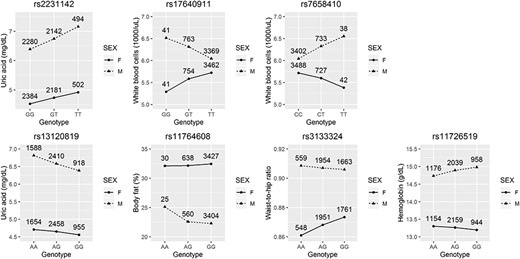
Identification of seven SNP-by-sex interactions
A total of three SNPs were detected to interact with sex at the genome-wide significance level of |$5\times{10}^{-8}$|, in which one was found on UA and two were detected on WBC (upper part of Table 2). With the two-step approach, additional four SNPs were identified to interact with sex on UA, BFP, WHR and Hb, respectively (lower part of Table 2). Figure 1 presents the interaction plots for these seven SNPs. Exploring individual SNP-by-sex interactions is challenging, because of the low power in detecting subtle interactions between sex and individual SNPs. Moreover, the multiple testing corrections would further compromise the statistical power.
SNPs detected to interact with sex
| Human complex traits | Stratum | SNP | Chromosome | Base pair | P-value of SNP-by-sex interaction |
|---|---|---|---|---|---|
| Detected at the genome-wide significance level of |$5\times{10}^{-8}$| | |||||
| UA | Younger (age |$\mathbf{\le}$| 50 y) | rs2231142 | 4 | 89 052 323 | 9.1E-9 |
| WBC | Elder (age > 50 y) | rs17640911 | 4 | 46 853 036 | 1.1E-8 |
| WBC | Elder (age > 50 y) | rs7658410 | 4 | 46 971 324 | 4.0E-8 |
| Detected according to the two-step approach | |||||
| UA | Younger (age |$\mathbf{\le}$| 50 y) | rs13120819 | 4 | 89 160 677 | 4.3E-7 |
| Body fat (%) | Elder (age > 50 y) | rs11764608 | 7 | 57 350 982 | 6.5E-7 |
| WHR | Elder (age > 50 y) | rs3133324 | 11 | 77 899 097 | 2.5E-7 |
| Hb | Elder (age > 50 y) | rs11726519 | 4 | 11 232 290 | 7.4E-7 |
SNP-by-sex interactions detected at the genome-wide significance level (|$5\times{10}^{-8}$|, top row) or by the two-step approach (bottom row).
The presence of PS-by-sex interactions in 18 out of 26 traits
As shown in Table 3, G |$\times$| S is significant in 18 traits for at least one age stratum (|${P}_{\mathrm{INT}}$| < |${$0.05$}\!\Big/ \!{$104$}\Big.=0.00048$|). Among 18 traits showing significant PS-by-sex interactions, most |${\hat{\phi}}_{\mathrm{INT}}$|s (Table 3) were in the same direction with |${\hat{\beta}}_F$|s (Table 1), except four anthropometric traits (BMI, BFP, WC and WHR), two blood-related traits (Hb and HCT [younger stratum]) and educational attainment (elder stratum). The most significant evidence of G|$\times$| S was found in WHR. Each 1 standard deviation (sd) increase in WHR–PS was associated with a 0.016 higher WHR in elder women than in elder men (|${P}_{\mathrm{INT}}$| = |$3.2\times{10}^{-55}$|), where 0.016 is approximately the length difference between the two bars in Figure 2F. Each 1 sd increase in WHR–PS was associated with a 0.011 higher WHR in younger women than in younger men (|${P}_{\mathrm{INT}}$| = |$1.1\times{10}^{-38}$|), where 0.011 is approximately the length difference between the two bars in Figure 2E.
Interaction between PS and sex on each complex trait (significant results with |${P}_{\mathrm{INT}}$| < |$0.05/104=0.00048$| are highlighted)
| Younger stratum (age |$\mathbf{\le}$| 50 y) | Elder stratum (age > 50 y) | |||||
|---|---|---|---|---|---|---|
| Human complex traits | Number of SNPs used to construct the PS | PS effect in females relative to malesa,b | |${P}_{\mathrm{INT}}$| | Number of SNPs used to construct the PS | PS effect in females relative to malesa,b | |${P}_{\mathrm{INT}}$| |
| Six cardiovascular-related traits | ||||||
| DBP (mmHg) | 15 | −0.204 | 1 | 3764 | −0.192 | 1 |
| SBP (mmHg) | 15 | 0.833 | 4.5E-02 | 399 | 0.954 | 3.2E-02 |
| TG (mg/dl) | 3842 | −2.295%a | 1.5E-03 | 810 | −1.365%a | 1 |
| Total cholesterol (mg/dl) | 415 | −2.085 | 8.1E-03 | 397 | 1.228 | 8.2E-01 |
| LDL cholesterol (mg/dl) | 423 | −2.294 | 4.7E-04 | 7193 | 0.521 | 1 |
| HDL cholesterol (mg/dl) | 765 | 1.530 | 1.4E-14 | 411 | 1.631 | 3.3E-11 |
| Two diabetes-related traits | ||||||
| FG (mg/dl) | 14 131 | −0.548%a | 8.2E-05 | 752 | −2.418%a | 2.7E-16 |
| HbA1c (%) | 7234 | −0.553%a | 6.8E-07 | 348 | −1.925%a | 1.2E-15 |
| Three kidney-related traits | ||||||
| Creatinine (mg/dl) | 1566 | 1.038%a | 4.5E-02 | 1503 | 0.559%a | 1 |
| UA (mg/dl) | 1575 | −0.223b | 3.6E-26 | 3649 | −0.139 | 9.4E-16 |
| BUN (mg/dl) | 742 | 1.453%a | 1.3E-02 | 72 | −0.782%a | 1 |
| Two liver-related traits | ||||||
| Total bilirubin (mg/dl) | 1496 | −1.369%a | 3.7E-01 | 3669 | −2.485%a | 1.4E-04 |
| Albumin (g/dl) | 3901 | 0.009 | 3.2E-02 | 51 | −0.009 | 7.3E-01 |
| Six anthropometric traits | ||||||
| Height (cm) | 7653 | −0.417 | 3.0E-05 | 1548 | −0.442 | 8.0E-04 |
| BMI (kg/m2) | 48 | 0.148 | 6.2E-01 | 765 | 0.241 | 1.9E-04 |
| Body fat (%) | 14 546 | −0.749 | 9.9E-29 | 14 606 | −0.660 | 3.6E-18 |
| WC (cm) | 416 | 0.913 | 1.2E-22 | 770 | 1.280 | 2.3E-41 |
| HC (cm) | 87 | 0.261 | 1.0E-02 | 1556 | 0.401 | 6.3E-12 |
| WHR | 780 | 0.011 | 1.1E-38 | 722 | 0.016 | 3.2E-55 |
| Five blood-related traits | ||||||
| RBC (million/uL) | 1533 | −0.035 | 6.6E-05 | 1532 | −0.049 | 2.3E-10 |
| WBC (1000/uL) | 3763 | 0.043 | 2.6E-01 | 3874 | −0.069 | 2.2E-03 |
| Platelet (1000/uL) | 1646 | 7.152 | 1.6E-15 | 3889 | 2.520 | 2.3E-03 |
| Hb (g/dl) | 1498 | 0.191 | 8.0E-14 | 837 | −0.153 | 6.4E-11 |
| HCT (%) | 1605 | 0.280 | 3.8E-04 | 876 | −0.412 | 6.6E-09 |
| Two other traits | ||||||
| Educational attainment (degree) | 375 | 0.023 | 9.2E-01 | 392 | 0.096 | 1.6E-05 |
| BSI | 831 | −0.995 | 3.5E-03 | 385 | −2.217 | 5.0E-12 |
aSix traits were natural log transformed, including TG, FG, HbA1c, creatinine, BUN and total bilirubin. For these six traits, |$(\exp ({\hat{\phi}}_{\mathrm{INT}})-1)\times 100\%$| is shown to represent the percent change in PS effect size between females and males. For example, each 1 standard deviation increase in TG–PS was associated with a 2.295% lower TG in younger women than in younger men (|${P}_{\mathrm{INT}}$| = |$1.5\times{10}^{-3}$|), where |${P}_{\mathrm{INT}}$| is the Bonferroni-corrected P-value for PS-by-sex interaction.
bFor other 20 traits, |${\hat{\phi}}_{\mathrm{INT}}$| is shown to represent the difference in PS effect size between females and males. For example, each 1 sd increase in UA–PS was associated with a 0.223 mg/dl lower UA in younger women than in younger men (|${P}_{\mathrm{INT}}$| = 3.6|$\times{10}^{-26}$|), where |${P}_{\mathrm{INT}}$| is the Bonferroni-corrected P-value for PS-by-sex interaction.
![The effect of PS on UA, WC and WHR. Sex-stratified regression model was built as $Y={\beta}_0+{\beta}_{\mathrm{PS}}\mathrm{PS}+\boldsymbol{\beta}_{\mathbf{C}}\mathbf{Covariates}+\varepsilon$, where Y is a trait, $\mathrm{PS}$ is the PS leading to the most significant gene-by-sex interactions, covariates have been described under model (1), and $\varepsilon$ is the random error term. Four regression models were built for each trait, regarding younger females (age$\le$ 50), younger males (age $\le$50), elder females (age $>$50) and elder males (age $>$50), respectively. The bars represent ${\hat{\beta}}_{\mathrm{PS}}$ on a trait, and the black segments mark the 95% confidence intervals, i.e. $\Big[{\hat{\beta}}_{\mathrm{PS}}-1.96\times \mathrm{standard}\ \mathrm{error}\ \mathrm{of}\ {\hat{\beta}}_{\mathrm{PS}},{\hat{\beta}}_{\mathrm{PS}}+1.96\times \mathrm{standard}\ \mathrm{error}\ \mathrm{of}\ {\hat{\beta}}_{\mathrm{PS}}\Big]$.](https://oup.silverchair-cdn.com/oup/backfile/Content_public/Journal/hmg/29/7/10.1093_hmg_ddaa040/1/m_ddaa040f2.jpeg?Expires=1750218541&Signature=aDRM7L4Dfn~LtBKmkd7~cEg2kYu8ONLLbRkUb51xz4VK4GSj~NwrPe2hl0wKVduCbe6qQ3CZ5XXPMHkNxPLM81RGpAs9qdaMLXjod0eYwybOYZ6wUYBKDFwl8D4Mp5XmVkP-r8I3ka0C~tKYQtwj0hnUgCM6HUpwngPWhkS0nKP27CJXR8oPF-3PJf1TT~xmp5jN2qGeW0swPRDKJNToVp4Psn4G70qobe58BPuyDe2bbhN-IFSousOIp8IQfPVwgX4unmcBPcROMBoKPfnvbw3qDsl6yJdn~E-UhDU~aUBjuAsCYIJhh9mjqUWrpFfIQXIjed8WsFJ-S1cjAQ7dsw__&Key-Pair-Id=APKAIE5G5CRDK6RD3PGA)
The effect of PS on UA, WC and WHR. Sex-stratified regression model was built as |$Y={\beta}_0+{\beta}_{\mathrm{PS}}\mathrm{PS}+\boldsymbol{\beta}_{\mathbf{C}}\mathbf{Covariates}+\varepsilon$|, where Y is a trait, |$\mathrm{PS}$| is the PS leading to the most significant gene-by-sex interactions, covariates have been described under model (1), and |$\varepsilon$| is the random error term. Four regression models were built for each trait, regarding younger females (age|$\le$| 50), younger males (age |$\le$|50), elder females (age |$>$|50) and elder males (age |$>$|50), respectively. The bars represent |${\hat{\beta}}_{\mathrm{PS}}$| on a trait, and the black segments mark the 95% confidence intervals, i.e. |$\Big[{\hat{\beta}}_{\mathrm{PS}}-1.96\times \mathrm{standard}\ \mathrm{error}\ \mathrm{of}\ {\hat{\beta}}_{\mathrm{PS}},{\hat{\beta}}_{\mathrm{PS}}+1.96\times \mathrm{standard}\ \mathrm{error}\ \mathrm{of}\ {\hat{\beta}}_{\mathrm{PS}}\Big]$|.
From Table 3, we can see that each 1 sd increase in WC–PS was associated with a 1.280 cm higher WC in elder women than in elder men (|${P}_{\mathrm{INT}}$| = |$2.3\times{10}^{-41}$|), where 1.280 cm is approximately the length difference between the two bars in Figure 2D. Each 1 sd increase in WC–PS was associated with a 0.913 cm higher WC in younger women than in younger men (|${P}_{\mathrm{INT}}$| = |$1.2\times{10}^{-22}$|), where 0.913 cm is approximately the length difference between the two bars in Figure 2C. Besides, Figure 2A and B shows sex-specific PS effects on UA, where highly significant evidence of G |$\times$| S was also detected. Each 1 sd increase in UA–PS was associated with a 0.223 mg/dl lower UA in younger women than in younger men (|${P}_{\mathrm{INT}}$| = |$3.6\times{10}^{-26}$|), where 0.223 mg/dl is approximately the length difference between the two bars in Figure 2A.
Discussion
Gene–environment interaction is defined as ‘a different genetic effect on phenotype in persons with different environmental exposures’ (11). Similarly, in this work, the presence of G |$\times$| S indicates a different genetic effect on complex trait ‘values’ in men and in women. Some previous studies transformed phenotypes within each stratum (men |$\le$| 50 year, men > 50 year, women |$\le$| 50 year and women > 50 year) (1,2) by mapping their within-stratum ranks to a standard normal distribution (4). These studies actually investigated whether genetic variants explain more/less ‘variance’ in one or the other sex. Supplementary Material, Table S1 presents our additional analyses on these rank normalized phenotypes. Except BFP, WC and WHR, all significant G |$\times$|S disappeared. This type of transformation removes heteroscedasticity in a phenotype between sexes. However, unequal phenotypic variability for the two sexes is a direct consequence of the presence of G|$\times$| S (proved in the Supplementary Material) (12,13). If we force the phenotypic variances for men and women to be equal, we may hardly detect different genetic effects on complex trait ‘values’ in men and in women.
Except anthropometric traits (1,2), few G |$\times$|S studies have been done for other traits. We used the PS-M approach (7) and provided a comprehensive investigation of sexual heterogeneity in autosomal genetic effects, for traits related to cardiovascular profiles, diabetes, kidney, liver, anthropometric, blood, etc. PS aggregates the effects among an ensemble of SNPs across the genome. Therefore, we cannot pinpoint specific genes or SNPs that interact with sex.
Because of less muscle, women on average have lower creatinine levels than men (14). Moreover, women have higher HDL-C (15,16) and lower TG (17) than men. Different gender roles in our society lead to lifetime systematic differences in environmental exposures for men and women. According to the Ministry of Labor of Taiwan, women are, on average, more risk averse than men in choosing occupations. Heavier works are generally performed by men. Moreover, across Asia, Europe, Africa and the Americas, men in general eat more meat than women (18), whereas women consume more fruits and vegetables (19). In our Taiwan Biobank (TWB) data, 5369 subjects aged under 50 and 4738 subjects aged over 50 completed the questionnaire regarding dietary habits. Consistent with most studies (18,19), our TWB data also show that women have a higher frequency in eating vegetables and a lower frequency in eating meat than men.
Because only a part of TWB subjects completed the dietary questionnaire, our regression analyses did not adjust for the dietary information. Compared with sex, information related to work, diet and environmental exposures is much more difficult to collect. Moreover, the validity of data regarding environmental factors is usually compromised by measurement errors and recall bias. In contrast, sex is a relatively unambiguous factor and can serve as a good surrogate for subtle environmental exposures.
For LDL-C and UA, the evidence of G |$\times$| S is much more significant in subjects aged under 50 years than in subjects aged over 50 years. The autosomal genetic effects of these two traits are weaker in women than in men. The evidence of G|$\times$| S in these two traits is diluted in the elder stratum. Estrogen might play a role in blunting the autosomal genetic effects of these two traits. Previous studies have found that estrogen could reduce the risk of cardiovascular disease (20–22) and was associated with lower levels of LDL-C (23–28) and UA (29). Our findings in Table 1 were in line with previous studies, where gender difference in these two traits is more notable in the younger stratum than that in the elder stratum. As shown in Table 3, our results show that estrogen might also play a role in attenuating the autosomal genetic effects of these two traits. For example, each 1 sd increase in LDL-C–PS was associated with a 2.29 mg/dl (|${P}_{\mathrm{INT}}$| = |$4.7\times{10}^{-4}$|) lower LDL-C in younger women than in younger men (Table 3). The evidence of G|$\times$| S on LDL-C was no longer significant in the elder stratum.
Studies have shown that estrogen can mitigate bone loss for postmenopausal women (30,31). Our results showed that women have lower BSI than men in both age strata, and the difference is especially prominent for subjects aged over 50 years (the last row of Table 1). Moreover, while the evidence of G|$\times$| S on BSI is not significant in the younger stratum, each 1 sd increase in BSI–PS was associated with a 2.217 lower BSI in elder women than in elder men (|${P}_{\mathrm{INT}}$| = |$5.0\times{10}^{-12}$|, the last row of Table 3).
Women in general have a healthier cardiovascular profile than men, including lower blood pressure levels, lower TG (younger stratum), lower total cholesterol (younger stratum), lower LDL-C (younger stratum) and higher HDL-C (Table 1). Moreover, women have lower values in FG, HbA1c (younger stratum), creatinine, UA, BUN and total bilirubin, where high levels in these traits are indicators of diabetes (FG, HbA1c), worse kidney function (creatinine, UA, BUN) and worse liver function (total bilirubin), respectively.
The genetic effects of some above-mentioned traits are weaker in women than in men, including: LDL-C (younger stratum), FG, HbA1c, UA and total bilirubin (elder stratum) (Table 3). Moreover, HDL-C is considered as ‘good cholesterol’ in the sense that higher levels of HDL-C are associated with a lower risk of heart disease (32). From Table 3, we can see that the genetic effects of HDL-C are stronger in women than in men. Each 1 sd increase in HDL-C–PS was associated with a 1.53 mg/dl higher HDL-C in younger women than in younger men (|${P}_{\mathrm{INT}}=1.4\times{10}^{-14}$|), and a 1.63 mg/dl higher HDL-C in elder women than in elder men (|${P}_{\mathrm{INT}}=3.3\times{10}^{-11}$|).
In this study, sexual dimorphism was observed in all the 26 complex traits (Table 1). Among these 26 traits, eight do not exhibit significant PS-by-sex interactions, including DBP, SBP, TG, total cholesterol, creatinine, BUN, albumin and WBC (Table 3).
Men and women have systematically distinct environmental contexts caused by hormonal milieu and their specific society roles, which may trigger different gene expressions even they have the same DNA materials. Although many subtle environmental factors are difficult to collect and quantify, sex can serve as a good surrogate for environmental exposures.
Materials and Methods
Taiwan biobank
The TWB aims at collecting genomic and lifestyle information from Taiwan residents aged 30–70 years (33, 34). Informed consent was obtained from all individual participants included in this study. Participants took a physical examination and provided blood and urine samples. Moreover, their lifestyle factors were collected through a face-to-face interview with one of the TWB researchers. All procedures performed in this study involving human participants were in accordance with the ethical standards of the Research Ethics Committee of National Taiwan University Hospital (NTUH-REC no. 201805050RINB) and with the 1964 Helsinki declaration and its later amendments or comparable ethical standards.
Our study comprised 20 287 TWB individuals who have been whole-genome genotyped until October 2018. To remove cryptic relatedness, we used PLINK 1.9 (35) to estimate the genome-wide identity by descent (IBD) sharing coefficients between any two subjects. Similar to many genetic studies (36–38), we excluded relatives within third-degree consanguinity by removing one subject from a pair with PI-HAT |$\ge$| 0.125, where PI-HAT = Probability (IBD = 2) + 0.5 |$\times$| Probability (IBD = 1). Finally, 18 425 unrelated subjects (9094 males and 9331 females) remained in the following analysis.
Most TWB subjects were of Han Chinese ancestry (33). The Axiom Genome-Wide TWB genotyping array was designed for Taiwan’s Han Chinese and was run on the Axiom Genome-Wide Array Plate System (Affymetrix, Santa Clara, CA, USA). In the TWB array, a total of 646 783 autosomal SNPs were genotyped. A total of 51 293 SNPs with genotyping rates < 95%, 6095 SNPs with Hardy–Weinberg test P-values < |$5.7\times{10}^{-7}$| (39), and 1869 variants with minor allele frequencies < 1%, were removed from our analyses. To adjust for population stratification, we used the remaining 587 526 SNPs to construct ancestry principal components.
10 traits obtained from physical examination or interview
Traits obtained from a physical examination included anthropometric profiles such as height, BMI, BFP, WC, HC and WHR. To have more reliable measurements, DBP of a subject was the average of two DBP measurements with a 5-min rest interval, and SBP was obtained similarly. BSI was measured as the bone exam result of an individual.
Educational attainment was obtained through a face-to-face interview with one of the TWB researchers. It was recorded as a value ranging from 1 to 7, with the following coding: 1: ‘illiterate,’ 2: ‘no formal education but literate,’ 3: ‘primary school graduate,’ 4: ‘junior high school graduate,’ 5: ‘senior high school graduate,’ 6: ‘college graduate’ and 7: ‘Master’s or higher degree.’
The sample sizes of these 10 traits obtained from physical examination or interview ranged from 17 849 (8787 males and 9062 females) to 18 425 (9094 males and 9331 females). The sample size of each trait can be found from Table 1.
16 traits obtained from blood or urine tests
Five traits related to blood were under consideration, including RBC, WBC, platelet, Hb and HCT.
Four traits related to lipids were investigated, including TG, total cholesterol, LDL-C and HDL-C. HDL-C and LDL-C are considered ‘good’ and ‘bad’ cholesterol, respectively. Numerous studies have demonstrated an inverse relationship between HDL-C and the risk of developing coronary heart disease (CHD) (40). Elevated LDL-C, elevated TG and low levels of HDL-C were causally associated with an increased risk of CHD (41).
Two traits related to diagnosis of diabetes, FG and HbA1c were analyzed. An HbA1c level higher than 6.5% can be used to diagnose diabetes (42). Moreover, according to the American Diabetes Association (43) and the Ministry of Health and Welfare in Taiwan, an FG level lower than 100 mg/dl is considered normal, an FG level between 100 and 126 mg/dl is prediabetes, and an FG level higher than 126 mg/dl is an indicator of diabetes.
Three traits related to kidney function were considered, including creatinine, UA and BUN. Creatinine is a chemical waste product produced by muscle metabolism and meat consumption. Because of more muscle mass and larger meat consumption (18), men generally have higher creatinine levels than women (Table 1). UA is a normal waste product made during the breakdown of purines. BUN is the amount of nitrogen in blood that comes from the waste product urea. In general, a BUN level around 7–20 mg/dl is considered normal. According to the Ministry of Health and Welfare in Taiwan, male creatinine higher than 1.4 mg/dl, female creatinine higher than 1.2 mg/dl, male UA higher than 7 mg/dl, female UA higher than 6 mg/dl and BUN higher than 20 mg/dl are all indicators of worse kidney function.
Two traits related to liver function, total bilirubin and albumin were under investigation. Bilirubin is a substance made during the normal breakdown of RBCs. Bilirubin passes through liver and is eventually excreted out of the body. A higher bilirubin level than the normal range (0.2–1.2 mg/dl) may indicate liver problems or an increased rate of destruction of RBCs. Moreover, according to National Institutes of Health, albumin is a protein made by liver. It carries various substances throughout one’s body, such as enzymes, hormones and vitamins. Lower than normal levels of albumin (3.8–5.1 g/dl) may indicate a problem in liver or kidneys.
The sample sizes of these 16 traits obtained from physical examination or interview ranged from 18 412 (9089 males and 9323 females) to 18 416 (9090 males and 9326 females). The sample size of each trait can be found from Table 1.
Definition of drinking, smoking and regular exercise
We here explain the definition of three covariates including drinking, smoking and regular exercise. In TWB, drinking was defined as a subject having a weekly intake of more than 150 cc of alcohol for at least 6 months and having not stopped drinking at the time his/her traits were being assessed. Smoking was defined as a subject who had smoked for at least 6 months and had not quit smoking at the time his/her traits were being assessed. Regular exercise was defined as engaging in 30 min of ‘exercise’ three times a week. ‘Exercise’ indicates leisure-time activities such as jogging, mountain climbing, yoga, etc.
Sexual dimorphism in complex traits
Six right-skewed traits were first natural log transformed before fitting the regression model (1), including TG, FG, HbA1c, creatinine, BUN and total bilirubin. The natural log transformation was widely used for these six traits in previous studies (45–50). Moreover, the R-square of model (1) was notably improved if these six traits were natural log transformed. Therefore, the natural log transformation was made on these six traits throughout all regression models in this study.
SNP-by-sex interactions in 26 traits
Notations have been described under models (1) and (2). By testing |${H}_0:{\beta}_{\mathrm{SNP},j}=0\ \mathrm{versus}\kern0.5em {H}_1:{\beta}_{\mathrm{SNP},j}\ne 0$|, we obtained marginal association P-value of the jth SNP with Y.
|${\hat{\beta}}_{\mathrm{SNP},j}$| (estimated from model (3)) and |${\hat{\gamma}}_{\mathrm{INT},j}$| (estimated from model (2)) are asymptotically independent under the null hypothesis of no SNP-by-sex interaction (proved in corollary 1 of (52)). A two-step approach that first filters SNPs by a criterion independent of the test statistic (|${\hat{\gamma}}_{\mathrm{INT},j}$| from model (2)) under the null hypothesis, and then only uses SNPs that pass the filter, can maintain type I error rates and boost power (51, 53).
Suppose there are L SNPs with marginal association P-values less than 0.1 (the largest P-value threshold in the following PS-M approach is 0.1, and therefore we also use 0.1 here). In the testing step, we fitted model (2) for these L SNPs. If the P-value of testing |${H}_0:{\gamma}_{\mathrm{INT},j}=0\ \mathrm{versus}\kern0.5em {H}_1:{\gamma}_{\mathrm{INT},j}\ne 0\ (j=1,\cdots, L)$| is less than the Bonferroni-corrected significance level of |$0.05/L$|, the jth SNP will be declared to interact with sex.
Polygenic scores of the 26 complex traits
The PS-M method (7, 8) was used to test the presence of G |$\times$| S for each of the 26 traits. This method incorporates a pruning stage and a filtering stage. We first pruned SNPs in high linkage disequilibrium (54,55), with the PLINK 1.9 command ‘plink —bfile TWBGWAS —chr 1-22 —indep 50 5 2’ (35). This means that we excluded SNPs with a variance inflation factor >2 within a sliding window of size 50, where the sliding window was shifted at each step of 5 SNPs. A total of 142 040 SNPs remained through this pruning step. Each trait or natural log transformed trait (denoted by Y) was then regressed on every SNP while adjusting for covariates, as described by model (3). Let |${P}_{\mathrm{SNP},j}$| be the P-value of testing |${H}_0:{\beta}_{\mathrm{SNP},j}=0\ \mathrm{versus}\kern0.5em {H}_1:{\beta}_{\mathrm{SNP},j}\ne 0$|, i.e. the significance of the marginal association of the jth SNP with Y (|$j=1,\cdots, 142\ 040$|).
|${\mathrm{SNP}}_j$| is the number of minor alleles at the jth SNP (0, 1 or 2). However, not all minor alleles are trait-increasing. Therefore, |${\hat{\beta}}_{\mathrm{SNP},j}$| in Eq. (4) can be positive or negative (|$j=1,\cdots, 142\ 040$|). A positive |${\hat{\beta}}_{\mathrm{SNP},j}$| indicates that the minor allele is trait-increasing, and a subject with more copies of the minor allele (more trait-increasing alleles) will have a larger |${\mathrm{PS}}_t$|. In contrast, a negative |${\hat{\beta}}_{\mathrm{SNP},j}$| represents that the minor allele is trait-decreasing, and a subject with more copies of the minor allele (more trait-decreasing alleles) will have a lower |${\mathrm{PS}}_t$|. Finally, a higher |${\mathrm{PS}}_t$| is linked to a larger trait value. Although ‘polygenic risk score’ or ‘genetic risk score’ is a commonly used terminology, we avoid inserting ‘risk’ into ‘PS.’ For some traits such as HDL-C and BSI, a higher PS is linked to a healthier profile.
PS-by-sex interactions in 26 traits
Let |${P}_{{\mathrm{INT}}_t}$| be the P-value of testing |${H}_0:{\phi}_{{\mathrm{INT}}_t}=0\ \mathrm{verus}\kern0.5em {H}_1:{\phi}_{{\mathrm{INT}}_t}\ne 0$|, where |$t=1,\cdots, 10$|. Because 10 tests have been performed, the Bonferroni-corrected P-value is |${P}_{\mathrm{INT}}=10\times \underset{t=1,\cdots, 10}{\min }{P}_{{\mathrm{INT}}_t}$|. The presence of G|$\times$| S will be declared if |${P}_{\mathrm{INT}}$| < |$0.05/104=0.00048$|, where 104 is the total number of tests performed in this study (26 traits |$\times$| 2 age strata, for sexual dimorphism tests [Table 1] and PS-by-sex interaction tests [Table 3], respectively). Although |$587\ 526$| SNP-by-sex interaction tests were performed for each trait, they were considered as the results of a benchmark method. Therefore, these |$587\ 526\times 26$| tests were not counted in our total number of tests.
Building PS with internal weights
Although the same data set is used to estimate |${\beta}_{\mathrm{SNP},j}$| from model (3) (|$j=1,\cdots, 142\ 040$|) and to test the significance of G |$\times$| S in model (5), this PS-M approach is valid in the sense that the type I error rates are satisfactorily controlled (7). Corollary 1 of Dai et al. (52) has justified the validity of using marginal associations (between SNP and a trait) as the filtering test statistics, and the data-splitting strategy is not required.
Building PS with internal weights has been widely used in gene–environment interaction analyses (7,8,51,59,61–63). Extracting weights from other cohorts or splitting data into two subsets is not required in the PS-M approach (7). The comprehensive simulations performed by Hüls et al. (61,62) and Lin et al. (7) have confirmed that building PS with internal weights is appropriate for detecting gene–environment interactions.
Acknowledgements
We would like to thank the anonymous reviewers for their insightful and constructive comments, and Mr Ya-Chin Lee for assisting with the acquisition of the TWB data.
Funding
This study was supported by the Ministry of Science and Technology of Taiwan (grant number MOST 107-2314-B-002-195-MY3 to Wan-Yu Lin). The acquisition of TWB data was supported by a MOST grant (grant number MOST 102-2314-B-002-117-MY3 to Po-Hsiu Kuo) and a collaboration grant (National Taiwan University Hospital: grant number UN106-050 to Shyr-Chyr Chen and Po-Hsiu Kuo).
Conflict of Interest Statement: The authors claim no conflict of interest.
