


SUMMARY
The global oceans are a noisy environment with characteristic acoustic and seismic soundscapes. The enclosed, sea ice-covered Arctic Ocean constitutes a particular noise environment that is rapidly changing. Here, we present a first, comprehensive description of the seismic soundscape of the Arctic Ocean recorded by ocean bottom seismometers especially equipped for the operation in sea ice. They were deployed at 4 km water depth in the Laptev Sea near the sea ice edge in September 2018 and recovered one year later. Analysis of the spectral power between 20 s and 60 Hz demonstrates that ambient noise levels are generally very low compared to other ocean bottom seismic records. Distinct noise bands at high frequencies (>6 Hz) characterize the winter time and are likely caused by the deformation of sea ice emitting seismic signals recordable at the ocean bottom over tens of kilometers. Sea ice noise decays suddenly in May while sea ice concentration is still 100 per cent, but freezing stops and compressional stresses decrease. It only gradually develops in autumn as sea ice becomes thicker, brittle and internally stressed. Microseisms with frequencies of 0.2–2 Hz appear with open water on the Laptev Shelf. Swell events in autumn cause large microseisms and high-frequency noise although ice-noise is not yet present in this season. Ice concentration decreases following the swell events, showing the impact of swell on the sea ice. Ocean bottom seismic records thus represent a powerful tool to monitor the interplay between wave action in the emerging Arctic Ocean and the physical state of its sea ice cover.
1 INTRODUCTION
The world's oceans are a noisy environment with a large variety of sound sources: sounds of biological origin like marine mammal calls, man-made noise caused by ship traffic or seismic surveys, and natural noise sources as wind and waves, earthquakes, volcanic activity, hydrothermalism or icebergs (see Bayrakci & Klingelhoefer 2023 and contributions therein). The ocean soundscape can be divided into an acoustic soundscape (Duarte et al. 2021) and a seismic soundscape (Diaz 2016). The acoustic soundscape is recorded by hydrophone moorings that capture pressure fluctuations in the water column from a lower frequency limit of 1–10 Hz to upper frequency limits in the kHz range (e.g. Dziak et al. 2013; Wilcock et al. 2014; Royer et al. 2015). These hydrophone arrays are typically moored in the sound fixing and ranging (SOFAR) channel in which sound can propagate over distances of thousands of kilometers (e.g. Dziak et al. 2012). In addition, hydrophone records also exist from the seafloor, often in combination with seismic records. The seismic soundscape of the oceans is recorded by ocean bottom seismometers (OBS) that record ground vibrations on the seafloor. This seismic soundscape extends to long-period signals covering roughly the range of 0.01–100 s (e.g. Diaz 2016). Ground vibrations recorded by OBS are only to a lesser extent produced by compressional waves travelling in the water column, but mostly of compressional, shear and surface waves that propagate below or along the seafloor. A certain overlap exists between the recording methods and the soundscapes. For example, blue whale vocalizations have been captured both by hydrophones and seismometers (Dunn & Hernandez 2009). Likewise, submarine earthquakes contribute to the seismic soundscape with P- and S-phases travelling below the seafloor and to the acoustic soundscape with T-phases propagating in the SOFAR channel (e.g. Bohnenstiehl & Dziak 2008).
Ocean microseism is the most dominant and ubiquitous signal of the seismic soundscape in the period range of 2–20 s (e.g. Bromirski et al. 2005; Beucler et al. 2015; Diaz 2016). Ocean microseisms are created by the interaction of ocean waves and the solid earth. They propagate mostly as Rayleigh waves and can be detected over thousands of kilometers. Different mechanisms have been suggested to explain how ocean waves produce energetic microseisms (e.g. Longuet-Higgins 1950; Haubrich & McCamy 1969; Ardhuin et al. 2015; Olinger et al. 2019). The description of the microseismic noise here follows the nomenclature of Bromirski et al. (2005): As ocean waves hit shallow shelf areas and shore lines, they produce seismic wavefields, the so-called single-frequency (SF) microseisms, with the same frequency as the exciting ocean waves. In the open ocean, double-frequency (DF) microseisms are created at half the period of ocean swell by nonlinear interaction of two wave fields travelling in nearly opposite directions, for example in the vicinity of powerful storms (e.g. Longuet-Higgins 1950; Ardhuin et al. 2015). Janiszewski et al. (2023) present a comprehensive review of ambient microseismic noise in OBS records. Away from coasts, the DF signal dominates the spectra, while SF noise is almost absent (Janiszewski et al. 2023). DF microseismic often displays two distinct bands, called long-period double-frequency (LPDF) and short-period double-frequency (SPDF) microseisms (e.g. Bromirski et al. 2005; Stutzmann et al. 2009; Diaz 2016). They are separated roughly at a frequency of 0.2 Hz (Bromirski et al. 2005). In particular the frequency range of the SPDF varies between ocean basins (Janiszewski et al. 2023). Near the coasts in shallow water, the SF signal is generally larger than the DF signal. The amplitude of ocean microseisms shows a seasonal variation with the stormier winter season producing stronger microseisms than the summer season (e.g. Aster et al. 2008).
At even lower frequencies (<0.03 Hz) infra-gravity (IG) waves (e.g. Crawford et al. 1991; Webb et al. 1991; Doran & Laske 2016) may be visible in spectra of OBS and pressure sensors. IG noise is mostly apparent in probabilistic power spectral density (PPSD) plots of the vertical component of broad-band OBS since tilt noise typically dominates horizontal component records (Janiszewski et al. 2023). In addition, whether IG noise is identifiable on OBS records or not is influenced by several factors, including sensor type, OBS design and in particular water depth: the period of IG waves depends on the water depth such that a so-called ‘noise notch’ clearly separates SF noise from IG noise for deep water OBS while it may be absent for shallow water stations and IG and SF signals form one pronounced peak. Yang et al. (2012) present instructive examples of clearly identifiable IG noise in PPSDs of vertical component OBS records both from deep and shallow water locations off New Zealand. In contrast, in PPSDs of Zhang et al. (2023), OBS self-noise overprints any likely existing IG signal. Webb et al. (1991) suggest that IG pressure fluctuations recorded at deep ocean sites result from long period wave energy generated at coastal areas within the ‘line of sight’ and may be blocked by topographic obstacles on the ocean floor.
The polar oceans exhibit a particular acoustic and seismic soundscape with specific sound sources related to the cryosphere: In the Southern Ocean, icebergs are a powerful source of both seismic and acoustic noise (see Schlindwein 2023 and references therein). Sea ice likewise emits acoustic noise as it deforms (e.g. Dziak et al. 2015; Duarte et al. 2021). Cook et al. (2020) give an overview of studies of the acoustic sound emissions of sea ice in the Canada Basin of the Arctic Ocean. Most of these studies were carried out in shallow water areas with hydrophones moored tens to few hundreds of meters below the ice pack. Acoustic ambient noise levels peak around 10 Hz beneath sea ice (Makris & Dyer 1986; Kristoffersen 2011). Noise is generated for example by thermally induced ice cracking or ice ridging as ice floes collide (see Cook et al. 2020 and references therein).
Since sea ice dampens ocean waves and hampers ocean swell generation (e.g. Wadhams et al. 1988), ocean microseisms are modulated by the annual sea ice cycle. The polar oceans therefore exhibit not only a particular acoustic soundscape but also a seismic soundscape that is affected by the sea ice cover. The polar oceans can serve as a natural laboratory to study the generation of ocean microseisms as the sea ice cover switches ocean noise sources on and off during the course of a year: Land-based seismic stations around Antarctica document a significantly reduced SF power in austral winter when sea ice blocks the shallow water coastal shelf areas (Stutzmann et al. 2009; Grob et al. 2011; Anthony et al. 2017; Cannata et al. 2019). Long-period DF signals in turn appear to result from more distant storms in the Southern Ocean and vary in strength throughout the year. However, they are not suppressed by sea ice since the sea ice cover does not extend to the typical source regions of long-period DF microseisms (Stutzmann et al. 2009). In the Arctic Ocean, the situation is reversed: The deep ocean basin is covered by more or less perennial sea ice. Ocean swell forms predominantly in shallow water shelf areas that become increasingly ice free as sea ice declines (Stopa et al. 2016). Tsai & McNamara (2011) exploit seasonal variations in the DF microseism power measured by land seismometers in the Bering Strait and off the Alaskan coast to infer the strength of the sea ice. Chen et al. (2025) can predict to a first order the seasonal variation in DF microseism power recorded at a coastal seismometer on Ellesmere Island for a period of 32 yr with a simple model of ocean wave activity and sea ice concentration.
All of these studies of ocean microseisms and its seasonal variations are based on data from land seismometers positioned near the polar coasts and thus do not reflect the seismic soundscape in the adjacent oceans. In general, considerably fewer studies exist that describe the seismic soundscape in the middle of the oceans far away from coasts (e.g. Webb 1998; Bromirski et al. 2005) compared to studies near shore lines, a general bias pointed out in the study of Janiszewski et al. (2023). To our knowledge no data set yet exists that could characterize the seismic soundscape in deep water areas of the Arctic Ocean over a full annual cycle. The main reason is that the deployment and recovery of OBS from sea ice covered waters requires advanced logistic efforts and bears a high risk of instrument loss. The difficulty in finding and recovering a freely rising instrument with rise times of about 1 h in dense ice fields drifting at up to 1 km h−1 and more has prevented any routine deployment of OBS. Krylov et al. (2021) tested OBS in shallow waters of the inner Laptev Shelf, but their data coverage is only about half a year, mostly in winter time. Recently Ding et al. (2022) conducted a wide-angle refraction seismic experiment at Gakkel Ridge with 43 OBS at the seafloor, but the recording time is less than 2 weeks and the seismic soundscape is dominated by active seismic data acquisition.
In this study, we present the first year-round OBS observation of seismic noise at a deep-water location in the Arctic Ocean. Our experiment was intended as pilot study mainly for testing OBS design and recovery strategies in sea ice. We deployed a small seismic network of broad-band OBS at Gakkel Ridge, roughly 500 km away from the slope of the continental shelf in the Laptev Sea, at water depths of about 4000 m (Fig. 1d). During August and September, this location is below the marginal ice zone. The remaining time of the year it is covered by dense sea ice (Figs 1a–c). This ice-covered deep-sea location adjacent to a seasonally ice-free shallow water fetch area for swell formation is highly interesting to further explore the provenance of ocean microseismic noise and its interplay with sea ice. In the emerging Arctic Ocean, wave action has hardly been studied (Thomson & Rogers 2014; Stopa et al. 2016), but swell events and storms especially in the freezing and thawing season are known to have a crucial impact on the sea ice cover and its properties like floe size distribution (e.g. Zhang et al. 2013; Kohout et al. 2014; Wang et al. 2016).
![Sea ice concentration at the OBS network location (star) around (a) deployment, (b) winter and (c) recovery time. Deep parts of the Arctic Ocean [1000 and 2000 m depth contours in black, Jakobsson et al. (2012)] remain ice-covered throughout the year. Triangle: nearest land seismic station TIXI. (d) Location of OBS stations (triangles) on Gakkel Ridge near the rim of Gakkel Deep (>5000 m water depth). Same stereographic projection as in (a)–(c). Bathymetry: Dreutter et al. (2023); sea ice concentration: Melsheimer & Spreen (2019).](https://oup.silverchair-cdn.com/oup/backfile/Content_public/Journal/gji/242/1/10.1093_gji_ggaf143/2/m_ggaf143fig1.jpeg?Expires=1750753188&Signature=PXvxf93hr~TR1GASdIumzpXw9DBTQ6z2e-UlGxMNGrzUF7BuDmQDJO7u4CdnSSDMLhjJWyafaaZRGqmzPyjFWFhXHAqzmMhk6CbSYbIa-1-UrE68OErA4DMspi63~GXpGYvTKycWVQ12yhFicsEojK0zDi1zVlw2SYYLREN1s-wZahNQDTB5RU7nP04E5z3X4lGQgX4M1FhvDTUUXz~-uUUMXmg3-RvDDiLbLqbFX6UUOx73Yls-GP4qouwLsnxvQ3E4Q3x1YQ53JILJDlEa0ZQWTKbnQFek-R1l3wAfcIxLeO6SGqoax5aCZmvbeQP3cgkVCYbhoMKd9UsW0AjELw__&Key-Pair-Id=APKAIE5G5CRDK6RD3PGA)
Sea ice concentration at the OBS network location (star) around (a) deployment, (b) winter and (c) recovery time. Deep parts of the Arctic Ocean [1000 and 2000 m depth contours in black, Jakobsson et al. (2012)] remain ice-covered throughout the year. Triangle: nearest land seismic station TIXI. (d) Location of OBS stations (triangles) on Gakkel Ridge near the rim of Gakkel Deep (>5000 m water depth). Same stereographic projection as in (a)–(c). Bathymetry: Dreutter et al. (2023); sea ice concentration: Melsheimer & Spreen (2019).
The geometry of our seismic network was optimized to record seismicity at a volcanic edifice at Gakkel Ridge providing first insights into the low-level seismicity of the ultraslow spreading Gakkel Ridge (Essing et al. 2025). Since the network consisted only of four stations spaced at about 8–20 km, advanced array processing techniques that allow for example for backtracking ambient noise sources (Pratt et al. 2017) were not applied to this data set.
The aim of this contribution is therefore to provide a comprehensive but qualitative description of the ambient seismic noise in Arctic deep-sea seismic records, highlighting the characteristics of the Arctic seismic soundscape over a spectral range of 0.02–60 Hz including artificial sources. The paper thus serves as a starting point and baseline observation for dedicated studies of ocean noise sources, and wave and sea ice interaction in the Arctic Ocean. Each noise source is described and discussed in individual chapters while the final interpretation and discussion mainly focuses on the annual noise cycle produced by sea ice and ocean swell and their mutual interaction.
2 MATERIALS AND METHODS
2.1. Ocean bottom seismometer operations in sea ice
We installed a trial network of four ocean bottom seismometers at eastern Gakkel Ridge near Gakkel Deep at about 82°N 119.5°E (Fig. 1). The network was deployed on 2018 September 15 during RV Polarstern cruise PS115/2 (Stein 2019) and recovered on 2019 September 27 during RV Polarstern cruise PS122/1a. The OBS of Lobster type with Trillium Compact seismometers (flat frequency response between 120 s and 100 Hz) and HighTechInc HTI-04-PCA/ULF hydrophones had been modified for ice operations following a prototype test in July 2014 during RV Polarstern cruise PS86 to western Gakkel Ridge (Boetius 2015). The OBS include a high-buoyancy conic head buoy with an integrated radio beacon. This head buoy is fixed to the OBS frame until release of the OBS. It is designed to force its way to the sea surface through ice slush (Fig. 2). In addition, the OBS is equipped with a Posidonia transponder to allow for accurate (about 5 m accuracy) ultra-short baseline acoustic tracking. This transponder is fixed to about 200 m of rope that is unspooled from a spindle upon release (Fig. 2). The transponder thus hangs vertically down from the OBS when it surfaces and can still be located accurately at horizontal distances of at least 150 m with the downward-looking (beam width 60°) Posidonia antenna in the hull of RV Polarstern. Although the sea ice consisted of small, soft ice floes and ice slush, the head buoy did not penetrate this ice and we had to rely on the position provided by the Posidonia transponder for tracking and recovering the OBS. The most efficient recovery strategy was to break ice at the expected surfacing position during the OBS rise time of about one hour. After surfacing, we circled the OBS position while continuously tracking the OBS until we could identify and break the ice floe retaining the OBS. All OBS were successfully recovered within 2 to 5 hr.
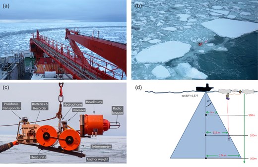
(a) Typical sea ice situation during recovery of the OBS. Ship track around the expected surfacing position of the OBS is visible. (b) OBS surfacing at the starboard side of the ship after ice breaking. Note that the head buoy did not surface. (c) Modified Lobster OBS design. Note the large head buoy and the transponder construction. (d) Concept of the OBS redesigned for continuous near surface tracking with the Posidonia system with the transponder hanging down from the OBS after release.
2.2. Data processing methods and further materials
The OBS yielded continuous data sampled at 250 Hz from 2018 September 16 until 2019 September 17. The hydrophone data were not usable due to amplification problems. The clock drift was determined from synchronization and noise cross-correlation (Hannemann et al. 2014), revealing some non-linear time drift, which was subsequently corrected. The orientation of the OBS could be determined to within 2 degrees from polarization of P waves from high quality records of teleseismic earthquakes (Scholz et al. 2017).
To assess the general noise conditions of the stations, we calculated PPSD plots (e.g. Figs 3 and 4) from the 250 Hz continuous waveforms with a window length of 3600 s using the method of McNamara & Buland (2004) as implemented in Obspy (Beyreuther et al. 2010).
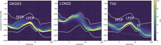
PPSD plots for 12 months of vertical component data from OBS GKD03 in the ice-covered Arctic Ocean, OBS LOK02 (Barreyre et al. 2023) in open waters of the Norwegian–Greenland Sea and land station TIXI (Laboratory/USGS, 2014). Grey lines: Peterson high- and low-noise model (Peterson 1993). See text for description of microseismic noise types SPDF, LPDF, SF.
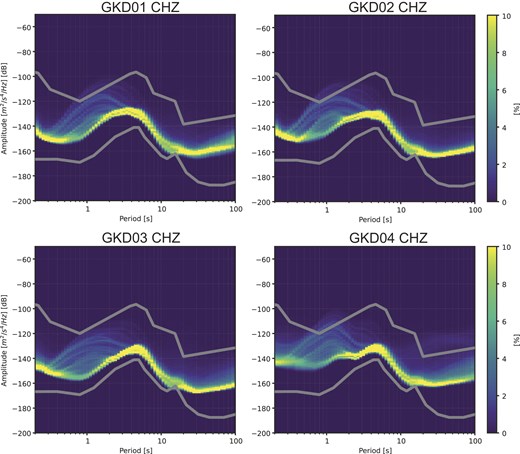
PPSD plots for 12 months of vertical component data from OBS GKD01-04. Grey lines: Peterson high- and low-noise model (Peterson 1993). Note the low noise level of station GKD03.
To resolve temporal changes of the ambient seismic noise, we additionally transformed our data into the time-frequency domain (e.g. Figs 5 and 6). The instrument response was removed, the signal decimated by a factor 2 and demeaned prior to calculating spectrograms of spectral power from 65.5 s long time windows using 213 = 8192 sample points for the Fast Fourier Transforms. The windows overlap by 10 per cent. Using the spectrogram function of Obspy (Beyreuther et al. 2010), we thus compiled a data base of spectra at 1 min intervals with a spectral resolution of 0.0159 Hz to also resolve more transient events. Depending on the signals of interest data were further averaged in time. Fig. 5 shows spectrograms of the vertical component of all four stations covering the entire year at a 30 min resolution. The electronic supplement contains data files (ds01-ds03) with high-resolution versions of the spectrograms for all stations and channels.
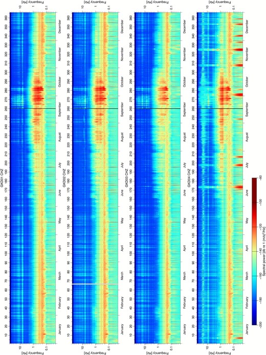
Spectrograms for the vertical channels of all stations. Vertical black line marks the start and end of the recording period with a discontinuity of the noise records across this line. Year 2018 right of black line, year 2019 left of black line. For enlarged versions and all channels see data files ds01-03.
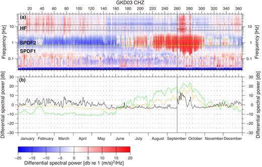
(a) Differential power spectrogram for the vertical component of GKD03. Black line: start of recording period in September 2018. Coloured boxes are frequency bands for determining the mean spectral power of the high-frequency signal HF and the SPDF microseisms. (b) Extracted differential spectral power over time for the marked frequency bands. HF and SPDF time-series are filtered with a cosine filter of 2 and 5 d full width, respectively.
For the subsequent description and analysis of the ambient seismic noise, we mostly rely on the vertical channel of station GKD03. This station showed the lowest overall noise levels (Fig. 4) being situated closest to the rift axis of Gakkel Ridge on the youngest and hardly sedimented seafloor compared to the other OBS positions, where a sediment cover was obvious in echosounder data.
To further enhance seasonal variations of the spectral power, we subtracted the annual mean spectral power of each frequency bin. Fig. 6(a) shows the resulting differential power spectrogram for the vertical component of station GKD03. To study in more detail the seasonal variations of ambient seismic noise, we extracted the spectral power in frequency bands of interest (Fig. 6), averaging the spectral power at all frequencies contained within the band. We thus obtained a time-series of spectral power per frequency band which we filtered by applying a cosine filter of full width of 2 d for the more variable HF signal and 5 d to enhance the longer period variations of the SPDF signals (Fig. 6b).
To compare the ambient seismic noise variations to the sea state and sea ice cover, we used maps of sea ice concentration retrieved from AMSR2 [Advanced Microwave Scanning Radiometer 2, www.seaice.uni-bremen.de, Melsheimer & Spreen (2019)] data using the algorithm of Spreen et al. (2008). The Arctic sea ice concentration grids have a resolution of 6.25 km by 6.25 km. We calculated the mean sea ice concentration within distances of 50 and 500 km from the OBS network, respectively, and thus obtained graphs of sea ice concentration over time with a daily resolution. Significant wave heights Hs and the primary wave mean periods Tp were obtained with a temporal resolution of 6 hr from the Wavewatch III® hindcast data set for the Arctic Ocean (Tolman 2009; Ardhuin et al. 2010). Average significant wave heights and mean wave periods were calculated for an area of 500 km radius around the OBS network and for different seas. We additionally used data of ice drift speed (OSI_SAF 2022) and ERA5 reanalyis data of 2 m air temperature (Hersbach et al. 2023) at the nearest available grid point to the OBS network on a daily resolution.
3 RESULTS: OBSERVATION OF AMBIENT SEISMIC NOISE AND DISCUSSION OF NOISE ORIGIN
The general seismic noise level in the Arctic Ocean is very low. Fig. 3 shows the probabilistic power spectral density plot of station GKD03 in comparison to OBS station LOK02 (same instrument type), placed at a geologically comparable location at the Knipovich–Mohns Ridge bend in the Norwegian–Greenland Sea in open water (Pilot & Schlindwein 2024), and to land station TIXI. Compared to TIXI, the OBSs show high noise-levels for periods longer than 20 s. At shorter periods, the noise level of station GKD03 is as low as land station TIXI close to the low noise model of Peterson (1993). For an oceanic environment this represents a very quiet seismic soundscape compared for example to the location of LOK02, where ocean microseism sources between 1 and 10 s exceed the high noise model. Even at periods <1 s, the open water location of LOK02 registers higher seismic noise levels than a sea ice covered location in the Arctic Ocean.
In the following paragraphs, we describe individual ambient seismic noise signals and their variability in time and discuss potential noise sources. We only shortly cover artificial noise sources, but focus our description on noise sources of natural origin.
3.1. Artificial noise sources
Artificial noise comprises distant noise sources such as ships or other anthropogenic noise and noise produced at the OBS for example as a consequence of ocean current acting on the structure of the OBS (Essing et al. 2021), OBS tilting, or sensor malfunctioning. Ship operations are likely to become a more prominent noise source in an increasingly ice-free Arctic Ocean. Since there is a prominent artificial HF noise signal on days 260–275 (Figs 5 and 6), we provide a description of noise signals that are potentially linked to OBS and ship-generated noise in Text S1 (Supporting Information).
3.2. Microseismic and IG wave noise
SF noise energy rapidly dissipates with depth such that SF noise is typically not seen at deep-sea OBS locations (Bromirski et al. 2005). During open water conditions in August, the PPSD plot of land station TIXI shows SF noise, whereas deep-water OBS station GKD03 has no SF noise peak (Fig. 7). During winter time, when the shallow water of the Laptev Sea shelf is covered by sea ice, SF noise is also weak for station TIXI.
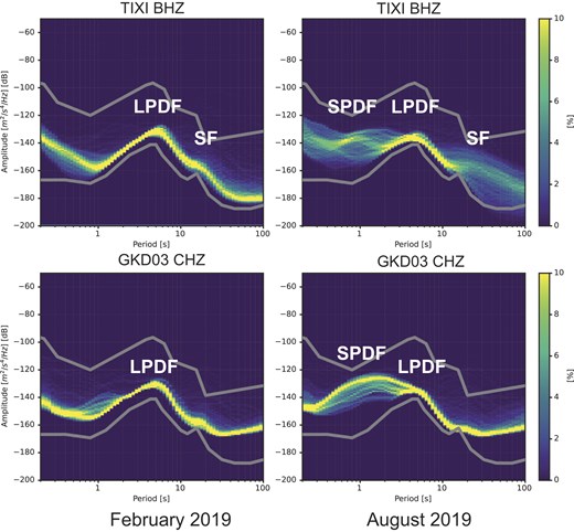
PPSD plots of vertical component data from land station TIXI and OBS GKD03 for February 2019 with sea ice cover in the Arctic Ocean and August 2019 during summer conditions. Grey lines: Peterson high- and low-noise model (Peterson 1993). See text for description of noise sources SPDF, LPDF and SF.
DF microseismic noise recorded in deep waters of the Arctic Ocean is clearly double-peaked and contains both LPDF and SPDF signals (Figs 3, 4 and 7) at distinctly different periods. The LPDF band reaches its maximum power at about 5 s, whereas the SPDF band shows a broad maximum between 1–2 s period. In contrast, station LOK02 (Fig. 3) in the Norwegian–Greenland Sea shows one broad DF peak of 2–5 s period, more in line with the shape of the bulk of the PPSDs in the comprehensive collection of Janiszewski et al. (2023).
An interesting observation is also the absence of a noise peak in the period band of IG waves at station GKD03. While station LOK02 in the Norwegian–Greenland Sea, equipped with the same sensor type, shows slightly elevated noise levels in the period range of >30 s (Fig. 3) and thus potentially some IG wave signal, we cannot fully rule out that OBS tilting obscures any IG waves at station GKD03. We have not attempted to remove tilt or compliance noise in this study to enhance IG signals (Janiszewski et al. 2023), due to malfunctioning of the hydrophones. Another explanation is that IG waves are indeed lacking or too weak to be prominently recorded at our deep water location. Bromirski et al. (2010) describe clearly identifiable IG waves in differential spectra from Ross Ice shelf, visible as dispersive events lasting for several days. Similar patterns are not observable in Fig. 6(a) in the IG noise band at periods >20 s. In the Arctic Ocean, wave buoys on the sea surface measured episodic IG waves at locations between 85°N and 87°N and 130°E with periods >19 s (Wadhams & Doble 2009). The sources of the IG waves were backtracked along a straight trajectory through the deep water passage in Fram Strait (Wadhams & Doble 2009; Ardhuin et al. 2016). Since a direct wave path is important for the observation of IG waves at the seafloor (Webb et al. 1991), the location of our seismic network at eastern Gakkel Ridge may be unfavourable for recording IG waves. We therefore limit our subsequent description to DF noise.
3.2.1. Long-period double-frequency microseismic noise (LPDF)
The LPDF band occupies the frequency range of 0.1–0.25 Hz corresponding to periods of 4–10 s (Figs 5 and 6a). This frequency range is consistent with the dominant global peak of LPDF around 0.14 Hz (Janiszewski et al. 2023). The width of the frequency band and its spectral amplitudes are higher during winter and lower during summer as illustrated by mostly blueish colours during the summer months in the differential spectrogram (Fig. 6a).
Especially during the winter time, individual LPDF events can be seen at frequencies between 0.1 and 0.15 Hz. Some of these events are dispersive with frequencies increasing over time. Similar time evolution of LPDF events has for example been observed by Diaz (2016) or Bromirski et al. (2015) and attributed to approaching storms as a moving source to cause dispersion. From qualitatively matching the timing of the LPDF events with hindcast plots of significant wave height, we can identify storm events in the Pacific Ocean and North Atlantic Ocean that likely cause the observed spectral signals (Fig. 8). Kedar et al. (2008) identified the southeast coast of Greenland (Fig. 8a) as a frequent and effective source area for the generation of deep microseisms that are recorded thousands of km away. The seasonality of the LPDF with higher noise amplitudes in winter agrees with observations by Stutzmann et al. (2009) who found from an analysis of noise spectra from land stations around the globe that the DF peaks in local winter. This yields further evidence that the LPDF signals observed at the bottom of the Arctic Ocean have their source outside the Arctic Ocean, since noise amplitudes are highest when wave action in the Arctic Ocean is inhibited by sea ice.
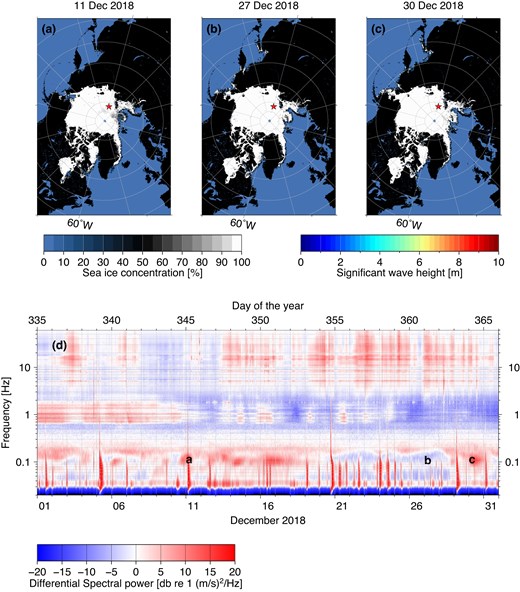
Sea state and ice conditions during (a) a swell event in the Atlantic Ocean, (b) calm conditions and (c) a swell event in the Pacific Ocean. (d) Differential spectrogram of GKD03 vertical channel marking the corresponding LPDF microseism events.
3.2.2. Short-period double frequency microseismic noise (SPDF)
The SPDF band appears very prominently in Figs 5 and 6 as time interval of high spectral power between about June and November occupying a frequency band between 0.13 and 1.7 Hz (periods about 0.6–7 s). Upon closer inspection, two components of this noise signal can be identified (Fig. 6a): The principal SPDF signal, now called SPDF1 signal, is best visible from August to October. Its lower frequency limit decreases to a minimum of 0.13 Hz at the end of September, overlapping with the LPDF signal. As for LPDF events, some dispersion is visible. The second component of the SPDF band, SPDF2, has slightly higher frequencies of about 0.7 to 1.7 Hz. Its frequency content does not vary with time, neither on seasonal scales nor within individual dispersive events. The signal starts before the main SPDF1 in June and lasts throughout November and December with some occurrences in late January and early February. It may be present throughout the summer overlain by the SPDF1 signal. Due its different signal characteristics we assume a different origin of the SPDF2. The seismic array of Pratt et al. (2017) in Antarctica detected microseismic noise in the same frequency band, which they term ultrashort-period microseism. They showed that the wavefield consists of body waves excited by distant storm systems and does not display a clear seasonality. A similar origin is likely here but our network does not have the capabilities to verify this explanation. Chen et al. (2025) observe strongly seasonally modulated SPDF noise from the Arctic Ocean in the period range of 0.5–2 Hz (2–0.5 s period) encompassing both SPDF1 and SPDF2 bands of our data.
To capture the individual evolution of the spectral power over time for these two SPDF components, we defined the extraction window for the SPDF1 from 0.13–0.64 Hz covering mostly its lower frequency part but staying clear of the SPDF2 signal, that we extracted between 0.64–1.7 Hz. The resulting variations of spectral power over time are shown in Fig. 6(b). The SPDF1 spectral power is to some extent contaminated by LPDF signal components in winter time, such that the lowest spectral power values in May and June are more representative for SPDF power also in the winter months. In general, SPDF power increases gradually from early June until mid-October and then rapidly drops to winter levels. Chen et al. (2025) observe the same seasonal modulation of their SPDF signal but with an abrupt increase in noise power at the start of the summer season followed by a more gradual decrease towards autumn.
Since SPDF microseisms in the deep ocean are proposed to result from swell in the open ocean (e.g. Bromirski et al. 2005; Stutzmann et al. 2009; Diaz 2016), we compared significant wave heights Hs and mean wave periods Tp in the Laptev, Kara and Barents Sea to spectral power and SPDF1 minimum frequencies (Figs 9a–c). The longest periods (or smallest frequencies) of the SPDF1 microseism should equal double the frequency of the exciting ocean waves, hence 2/Tp. For the purpose of this study, we defined the Barents Sea from 15°E to 60°E, the Kara Sea from 60°E to 93.4°E and the Laptev Sea from 93.4°E to an ice tongue near 165°E (Fig. 9d). The comparison shows a close match for the Laptev Sea for Hs and 2/Tp, but no similarities between the SPDF1 temporal variations and wave action in the Kara or Barents Sea. The time-series characterizing the wave action are dissimilar between the three seas and cannot easily be matched by a time lag caused by a moving storm system. Instead, swell development appears rather local, such that we can qualitatively identify the source region of the observed SPDF1 in the Laptev Sea. Fig. 9(a) distinguishes between the swell in the entire Laptev Sea area and only the deep-water area within 500 km of the OBS. The variation of spectral power over time matches better the significant wave height averaged over the entire Laptev Sea area compared to the significant wave height in the 500 km deep-water area. The latter displays considerably higher maxima during three swell events on days 271, 280 and 282 that do not lead to equally prominent peaks in the noise power. In contrast, the SPDF1 lower frequency limit is better explained by mean wave periods in the deep-sea portion of the Laptev Sea which show more pronounced variations over time than the larger area including the shallow shelf.
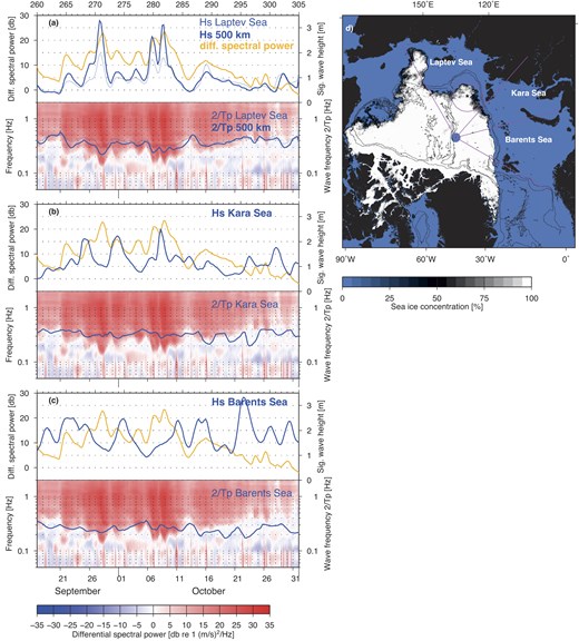
(a)–(c) Top panels: Time-series of SPDF1 differential spectral power and significant wave heights for areas outlined in (d). Bottom panels: Close-up of spectrogram (Fig. 6) showing minimum frequency of SPDF1 band overlain with the same quantity calculated from the mean wave period in the areas in (d). (d) Areas used for calculating average Hs and Tp. Circle is 500 km radius from OBS (star).
3.3. Sea ice noise
At frequencies above 3 Hz, increased spectral power dominates the winter season from about mid-November until mid-May (Figs 5 and 6a). The noise signal appears as vertical blocks or thin lines in the spectrograms covering a frequency range of 3 Hz to at least 60 Hz. The signal blocks occur simultaneously at all stations (Fig. 5) of the network, such that the same signal is perceived in an area of roughly 10–20 km extent. However, individual seismic events that could be responsible for the increased spectral power could not be identified in the waveform data. We therefore assume that the source of the signal is not local, that is, immediately above the individual seismic stations. In such a case, differences in the temporal occurrence pattern between individual seismic stations would be expected along with sharp, identifiable local seismic events. Instead, we assume that the signal is produced at distances of the order of several tens of kilometers, travels as a seismic wave in the subsurface and the same seismic wavefield is observed across our network.
We assume that the source of this HF noise is related to the sea ice. Icequakes in sea ice, recorded by seismometers on ice floes (Läderach & Schlindwein 2011), release seismic energy in a frequency range matching our ocean bottom observations. The deformation of sea ice radiates energy into the water column: Wilcock et al. (2014), summarizing earlier studies on the acoustic soundscape of ice-covered oceans, state that the frequency range below 100 Hz is strongly contaminated by noise of cracking and deforming sea ice. Temperature induced cracking of sea ice is observed locally (<10 km distance) at frequencies higher than about 60 Hz (Milne 1972; Stein et al. 2000) and can thus not explain our observations. According to Makris & Dyer (1986), noise correlating with stress in the ice pack peaks at about 10 Hz. Acoustic noise attenuation is low in the frequency band of 10–30 Hz, such that sea ice ridging at distances of several tens of km is assumed to cause a broad frequency peak centred around 20 Hz with thicker ice producing louder ridging noise (Buck & Wilson 1986; Greening & Zakarauskas 1991; Cook et al. 2020). Although all of these observations are made either with hydrophones or seismometers immediately on or just below the ice, we speculate that the acoustic energy released by sea ice deformation is high enough to reach the seafloor and convert into a seismic wave travelling in the subsurface. In the absence of concurrent seismic measurements on ice floes or individual, identifiable and locatable seismic events, a direct connection between seismic sources in the sea ice and ocean bottom records cannot be made.
To assess the temporal variation of the high-frequency signal, we averaged the spectral power between 6 and 13 Hz as a representative but arbitrarily chosen frequency band, extracted its time-series (Fig. 6b) and compared it to time-series of sea ice drift speed, air temperature and sea ice concentration within 50 km distance from the OBS network (Fig. 10d). Rapid variations of the spectral power of high-frequency noise on the order of days are not related in a systematic way to variations in air temperature, drift speed or ice concentration. For example, thermal ice cracking happens when air temperatures drop (e.g. Cook et al. 2020 and references therein), but no relation between increased noise power and cold days is observed, confirming that thermal cracking is an unlikely source for the HF noise. Likewise neither local ice drift speed nor large changes in drift speed appear to systematically cause peaks in HF spectral power. This suggests that the stress state of the sea ice cover requires a more comprehensive physical description likely on a much larger scale to elucidate potential links to the HF spectral power. However, this is beyond the scope of this descriptive manuscript of the seismic soundscape of the Arctic Ocean.
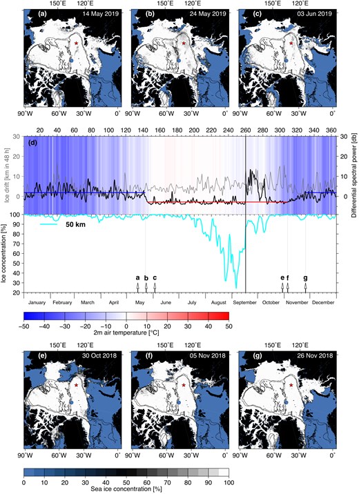
(a)–(c) and (e)–(g) Sea ice concentration from AMSR2 data (Melsheimer & Spreen 2019) on dates marked in (d). Star: OBS location. (d) Differential spectral power in HF band (black line) with winter (blue horizontal line) and summer (red horizontal line) average HF noise levels, vertical lines mark start and end of HF noise periods. Grey: ice drift speed (OSI_SAF 2022), coloured background: 2 m air temperature (Hersbach et al. 2023). Bottom panel: average sea ice concentration within 50 km of the OBS.
On a seasonal scale, the HF spectral power time-series displays two levels: a winter level, calculated from averaging the spectral power from December to April and a summer level (June–August). Spectral power variability around this level is significantly higher in winter time than in summer (Fig. 10d). Spectral power drops within 2 d starting on 2019 May 23 to summer level, concurrent with the last days of freezing. Sea ice concentration in vicinity of the OBS (50 km) remains near 100 per cent until July (Fig. 10d), but small patches of open water form in the Laptev Sea (Figs 10a–c) during the rapid transition to summer noise levels. The transition to winter noise levels takes about three weeks, starting roughly on 2018 November 5. Freezing in the area started already in September and local sea ice concentration reached 100 per cent by mid-October, but a rapid closing of the last open water patches in the Laptev Sea (Figs 10e–g) happens early in November. These observations suggest two explanations for the generation of HF seismic noise that are not mutually exclusive but potentially complementary: (1) The sea ice changes its physical properties rapidly as freezing stops and melting sets in and it quickly looses its mechanical strength. The newly formed ice in autumn needs sufficient time to gain enough thickness and mechanical strength for failure in icequakes. (2) The ice cover of the entire Arctic Ocean gets under internal compressional stresses as sea ice cover reaches the coasts, such that ridging events become frequent. Stress measurements by Richter-Menge et al. (2002) in the Beaufort Sea give indications for a similar behaviour: internal stresses increase when freezing closes seasonally open water areas between the coasts and the perennial ice zone. They further describe a spiky nature of the stress record with events of internal stress lasting for several days, related to persistent wind forcing or other conditions producing convergence. A hypothetical explanation for the distinct noise levels observed in this study is that the first mechanism contributes to the generally higher mean HF noise level in winter, while the second mechanism causes the greater temporal variations about this mean in winter time.
A further interesting aspect is the difference in winter and summer noise levels between the acoustic and seismic soundscapes: the acoustic soundscape (10–1000 Hz) is quieter during the winter months and loudest between May and October (Cook et al. 2020), just opposite to the seismic soundscape in the HF band. An explanation is that sources of acoustic noise, like waves impinging on ice floes, wind, mobile ice floes rubbing against each other, produce acoustic noise but no seismic noise that could be felt on the deep seafloor. These loud acoustic noise sources are suppressed in a totally ice covered ocean in winter. In contrast, seismic HF noise likely reflects powerful sea ice deformation events that require a frozen ocean ideally under compression.
4 INTERPRETATION: SEASONAL VARIATIONS OF THE ARCTIC SEISMIC SOUNDSCAPE REFLECT SEA ICE AND WAVE CONDITIONS
Our records of ambient seismic noise at the ocean bottom of the Arctic Ocean showing both sea ice-related HF noise and swell-induced SPDF noise give interesting insights into the seasonal states of the Arctic sea ice and wave action and their mutual influence. We describe and interpret the Arctic seismic soundscape in the following in several phases (Fig. 11):
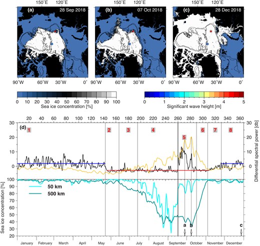
(a)–(c) Sea ice concentration (Melsheimer & Spreen 2019) and significant wave height (Ardhuin et al. 2010) on dates marked in (d). Star: OBS location. (d) Differential spectral power in HF and SPDF1 band. Horizontal lines: average HF noise levels in winter (blue) and summer (red); vertical lines mark start and end of numbered phases described in the text. Average sea ice concentration within 50 km (deep-sea area) and 500 km (also shallow Laptev Shelf) of the OBS.
Phase 1 and 8 represent the winter conditions. The Laptev Sea is entirely frozen, swell is completely suppressed and even pronounced storms in the Barents Sea (Fig. 11c) produce no SPDF1 signal at the OBS location in the Laptev Sea, confirming a local generation of SPDF1 noise. The sea ice cover in these phases is mechanically strong and potentially under internal compressional stress releasing considerable seismic energy into the water column recordable at deep-sea OBSs. In Phase 2, the sea ice-cover loses its mechanical strength and/or its internal stress within few days revealed by the mean HF spectral power rapidly dropping to summer levels. At this time, the sea ice concentration in the entire Laptev Sea area and particularly around the OBS is still near 100 per cent (Figs 10a and 11d), such that the change in HF power level is unlikely to result from a decrease of collisions between ice floes in the wider area of the OBS, but rather represents a change in the physical properties of the sea ice cover or a loss of its internal stress as the first tiny patches of open water emerge (Fig. 10c). In phase 3, the fetch area for swell in the shallow shelf area of the Laptev Sea starts to form (Fig. 11d). At the same time, SPDF1 power starts to increase from the lowest levels in phase 2, although the OBS location is still ice-covered. This shows that some SPDF1 signal can be created in shallow water areas and propagate over distances >500 km to the deep-water OBS location. Phase 4 describes the summer conditions. The OBS is now situated below the marginal ice zone. With increasing fetch area, the mean period of the swell increases as evidenced by decreasing SPDF1 minimum frequencies (c.f. Fig. 9a). The noise levels in the HF band, however, remain constant throughout phase 2–6 although the sea ice concentration varies drastically, suggesting that the summer HF noise levels are not a function of sea ice concentration.
In late September (day 271) and early October (days 280–282), large storms pass the Laptev Sea (phase 5, Figs 11b and c). Since the fetch area is still large, long-period waves can form (Figs 6 and 9a). They also affect the sea ice concentration, which had been building up already near the OBS location but drops as a consequence of the storms. Interestingly, these swell events are connected with considerable power in the HF band, deviating strongly from the summer power level. These noise events are partially overprinted by the ship-induced noise, but can be distinguished from the latter by a more gradual onset and decrease (Text S1, Supporting Information). This also discriminates these swell-related HF events from the sharper-bounded and shorter winter HF bands caused by sea ice deformation (Fig. 6a). We speculate that storm-induced collisions and break-up of sea ice still is the source of the HF noise. An explanation for the different appearance of the noise blocks is that the distance to the noise source is larger and signals become more attenuated. The observation that blocks of increased HF power occur simultaneously at the OBS stations suggests that the source region of the HF signal extends over at least several tens of km and may thus reflect storm-induced collisions of distant ice floes. For the storm in September, the OBS is located near the ice edge and the distance to more solid noise-producing ice floes may be larger than in winter time. For the events in October, the OBS location is already covered to 100 per cent by sea ice suppressing local wave action. In this case, colliding ice floes may also be some distance away. Another explanation for the different signature of the HF noise could be differences in the mechanical strength of the newly forming sea ice and the winter sea ice. Another source of swell-related noise could be the breaking of waves causing bubbles in the water column, but this noise is typically seen at considerably higher frequencies on hydrophones (Wilcock et al. 2014).
After the passage of the early October storms, the Laptev Sea freezes rapidly and SPDF power decreases constantly in phase 6. Like in phase 3, SPDF1 power is present although the fetch area is limited to the shallow Laptev Shelf. The spectral power drops at the same pace as freezing progresses and the fetch area shrinks. This suggests that already the young sea ice can efficiently suppress ocean swell while not yet emitting HF deformation noise. Phase 7 starts as 100 per cent ice concentration is reached. SPDF power is now absent and HF power levels build up gradually over a period of 20 d. As discussed previously, likely explanations are that the sea ice needs to become mechanically strong and sufficiently thick to produce icequakes by brittle failure, and internal stresses in the ice cover may increase as freezing reaches the coasts and stress events cause ridging that may produce seismic energy recordable at distant deep-water seismometers during the winter phase 8.
5 CONCLUSIONS
We presented the first records of ambient seismic noise at the bottom of Arctic Ocean over a full season and described the seismic soundscape of the Arctic Ocean and the temporal variation of its noise sources. By comparison with environmental parameters like ocean wave heights, air temperature or sea ice concentration, we identified the following noise sources in different frequency bands:
LPDF microseisms (0.1–0.25 Hz) are caused by wave action outside the Arctic Ocean. They are stronger in winter time and not modulated by the annual sea ice cycle.
IG waves (<0.05 Hz) could either not be resolved or were absent at our recording location.
SPDF microseisms (0.13–1.7 Hz) are generated by swell in the Laptev Sea area. Variations of the SPDF spectral power and minimum frequencies on a daily scale match the variations of significant wave height and mean wave periods in the Laptev Sea. The seasonal variation of the SPDF noise power is closely related to the sea ice concentration and the size of the fetch area in the Laptev Sea. SPDF power is also present when the fetch area comprises only shallow water areas of the Laptev Shelf.
Sea ice is the likely cause for high-frequency (>6 Hz) noise that is especially apparent in winter time with noise events lasting on the order of few days. We assume that sea ice deformation like for example ridging not only produces acoustic signals recorded by hydrophones below the sea ice, but emits sufficient seismic energy to be recorded at the sea floor over a distance of at least several tens of kilometers. Sea ice noise power drops to lower summer levels within about 2 d concurrent with the last days of freezing and the first appearance of open water at the shores of the Laptev Sea. Winter noise levels build up over a period of three weeks after the sea ice cover has reached the coast of the Laptev Sea. We propose that the HF noise reflects the mechanical strength of the sea ice and its internal stress state. However, a direct link between seismic signals at the sea floor and their seismic source processes in the sea ice cannot be established with the means of this study.
Of particular interest is the relative timing of SPDF and HF noise, characterizing swell and sea ice that mutually depend on each other as sea ice suppresses wave action. On shorter timescales, the passage of individual autumn storms can be monitored that directly impact the newly forming sea ice and cause HF noise. The appearance of this HF noise, however, differs from the typical winter HF noise, potentially due to a larger distance to noise sources or a different physical state of the surrounding sea ice.
Long-term installations of broad-band ocean bottom seismometers may thus represent a new and complementary way to monitor the state of the Arctic Ocean cryosphere from below at fixed locations. As sea ice further recedes and the Arctic Ocean becomes increasingly ice-free, pronounced changes of the seismic soundscape can be expected. OBS records can synchronously monitor the wave action of the emerging Arctic Ocean and the condition of its sea ice cover as its strength, composition and stress state change. To optimally profit from sub-sea ice OBS records, a direct link between the seafloor HF seismic signals and the physics of the overlying sea ice needs to be established, ideally by concurrent multiparameter measurements on the sea ice to reveal the source processes of HF noise on the Arctic seafloor.
ACKNOWLEDGEMENTS
The authors thank crew and scientists of Polarstern cruises PS115/2 and PS122/1a. J.-R. Scholz and M. Hiller are thanked for their aid in deploying and developing the OBS. The Editor J. R. Hopper, L. Bie and an anonymous reviewer provided helpful comments to improve this manuscript. Funding: Shiptime was granted under Alfred-Wegener-Institut Helmholtz-Zentrum für Polar- und Meeresforschung Grant No. AWI_PS115/2_01. OBS were provided by the DEPAS Pool (Alfred-Wegener-Institut 2017). We acknowledge support by the Open Access publication fund of Alfred-Wegener-Institut Helmholtz-Zentrum für Polar- und Meeresforschung.
AUTHOR CONTRIBUTIONS
VS (Conceptualization, funding, data curation, formal analysis, investigation, supervision, writing original draft), SL (Formal analysis, investigation, writing review), HK (Conceptualization, resources) and MS (Funding, data curation, methodology, writing review).
DATA AVAILABILITY
Raw, continuous seismic data of stations GKD01-04 are available from PANGAEA (Schlindwein et al. 2022b), 10.1594/PANGAEA.947045, time-corrected miniseed data from GEOFON network code 8F (Schlindwein et al. 2022a), 10.14470/3S7563492742. We further used seismological data from stations LOK02 (Barreyre et al. 2023), 10.14470/3Z326135, KNR03 (Schlindwein et al. 2018), 10.1594/PANGAEA.896635 and TIXI (Laboratory/USGS 2014), 10.7914/SN/IU. Figures were prepared with GMT4 and 5 (Wessel et al. 2013). Seismological data were processed with Obspy (Beyreuther et al. 2010).
