SUMMARY
Central to the task of seismic hazard assessment is the evaluation of potential amplifications due to site effects. The horizontal-to-vertical spectral ratio (HVSR) of ambient seismic noise (ASN) is a widespread measurement to assess the predominant soil frequency of a given site and estimate the wave velocities of the subsoil stratigraphy using inversion schemes. In practice, the inversions are currently made, assuming flat layers. In fact, HVSR measurements may show significant lateral and azimuthal changes due to the spatial variations of local geology, which can introduce uncertainties into the characterization of a site. This suggests the importance of considering detailed measurements of lateral and angular variations in layered settings. Inversion of soil properties at depth for horizontally layered media has become feasible assuming that ASN constitutes a diffuse field, that is, produced by equi-partitioned uniform illumination and/or by random sources and the ensuing multiple scattering by heterogeneities. Under the diffuse field assumption (DFA), the HVSR have been modelled by calculating the imaginary parts of the Green's function (IMGs) when source and observer coincide at the same point. In this work we use the 3-D indirect boundary element method (IBEM) to model the HVSR for each independent horizontal direction referred to here as directional-HVSR for layered media with lateral inhomogeneity. The IMGs at the source required to get HVSR have locality properties that depend on frequency and may imply significant economies in the calculation. For simple models we modelled the IMGs approximately using an adaptive meshing scheme that accounts both for the locality of the problem and the diffraction properties of waves at low and high frequencies. The obtained directional-HVSR displays variations in both frequency and azimuth. The results also show that layer interface variations can lead to ‘spots’ of higher wave excitation associated to local resonant modes. This shows the importance of HVSR in forecasting earthquake response and suggests the need for denser field measurements to study lateral and azimuthal variability. In order to show the reality of directional-HVSR, field data from Chalco, a soft soil site at the southern part of the Valley of Mexico, have been preliminarily analysed.
1. INTRODUCTION
The main goal in earthquake resistant design is to obtain design spectra of structures such that they withstand strong earthquakes. A crucial ingredient in this task is to evaluate the site effects through seismic characterization of the site. This complex issue needs to be simplified in order that practical measures could be at the reach of practitioners such as the predominant soil frequencies and the wave velocities of the soil profile to compute amplification factors.
In Japan, the tradition of studying microtremors dates back to the first half of the 20th century. Microtremors originate by the interaction of the ocean waves and the solid earth, by wind and by human activity as well. Here we call them ambient seismic noise (ASN). Kanai (1983) measurements in the 30s displayed the predominant frequency or period of a site by counting zero crossings in his smoked glass recordings. Nogoshi & Igarashi (1971) first computed the horizontal-to-vertical spectral ratio (HVSR or ), but their findings received little attention. It was Nakamura (1989) who proposed to use the HVSR to assess the predominant frequency of a site. He went farther and proposed HVSR as a proxy of transfer function to be used to compute the site effect. Nakamura's proposal was rapidly considered around the world mostly by engineers. For example, the SESAME European Research Project (2004) led a significant research effort.
On the other hand, the early 21st century has experienced a boom in passive seismology based on the formalization of the pioneering studies of Aki (1957) and the discoveries of Weaver (1982, 1985), which produced spectacular results in experimental (Weaver & Lobkis 2001) and field (Hennino et al. 2001; Campillo & Paul 2003) studies, in regional tomography (Shapiro et al., 2005) and exploration seismology (Schuster 2009). ASN is crucial to construct virtual sources in exploration seismology. In some circumstances, when the field is not completely diffuse, weighting approaches may enhance the diffuse field characteristics (Weaver & Yoritomo 2018; Piña-Flores et al. 2021).
Weaver (1982, 1985) formulated, four decades ago, the diffuse field theory in dynamic elasticity. This theory asserts that, within a diffuse field the average of cross-correlation is proportional to the imaginary part of the Green's function (IMGs) (Sánchez-Sesma & Campillo 2006; Sánchez-Sesma et al. 2008). In the same way, the average autocorrelations are proportional to the IMGs when source and receiver coincide. This fact is associated with the partitions of energy among states or modes (Perton et al. 2009) and exact deterministic results (Miller & Pursey 1955; Sánchez-Sesma et al. 2011a). Under the diffuse field assumption, Sánchez-Sesma et al. (2011b) modelled the HVSR of ASN for horizontally layered medium in terms of the IMGs when source and receiver coincide at the point of interest, and its inversion allowed to retrieve vertical profiles of mechanical properties (see García-Jerez et al. 2016; Piña-Flores et al. 2017, 2024) even for borehole recordings and for offshore and lake sites with an uppermost water layer (see Lontsi et al. 2015, 2019). Molnar et al. (2022) give a complete account of HVSR.
Additionally, the horizontal ASN may show azimuthal variations which may influence HVSR results, these polarizations have been attributed to fault-induced cracking, topographical effects and even anisotropy (see Pischiutta et al. 2017). Matsushima et al. (2014, 2017) explored the HVSR of a varying layer profile at Uji, Kyoto, Japan and Onahama, Tohoku, Japan, respectively, where several measured points allowed detecting significant differences in the HVSRs for independent horizontal components. In those cases, the spectral element method (SEM) was used to compute the response in time domain and the IMGs were computed by Fourier analysis of data close to the loading point. The exercises were not formal inversions, but the numerical modelling showed significant improvement in the matching of calculations with observations when the known structure was accounted for. Similarly, Perton et al. (2017) modelled the lateral variations at the Ijen volcano, Indonesia, taking advantage of the exposed layers at the crater rim.
Looking to understand and model these cases, we studied a flat layer over a half-space using the 3-D indirect boundary element method (IBEM) adapting the formulation by Sánchez-Sesma & Luzón (1995) and Perton & Sánchez-Sesma (2015) to compute the system IMGs directly in frequency domain. The IBEM in 3-D is not too restrictive regarding absorbing boundary conditions. In fact, we left open the layer sides and the underlying half-space was modelled only by a finite flat surface. The HVSR for a single layer is obtained almost as fast as the analytical modelling in cylindrical coordinates. Results reveal the crucial role of diffraction at low frequencies and the asymptotic ray behaviour at high ones. They also show the strong local behaviour of the IMGs ;at a point.
Furthermore, we studied two cases of a layer over a half-space with smooth lateral variations of the interface. The localized behaviour close to the observation point also exists in these varying profiles (the number of equations to solve is no longer constant, but it shows small variations). Our strategy is to compute the system IMGs at a single point implementing an adaptive mesh whose element sizes diminish with frequency as required for wavelength resolution. In this sense, we use large elements and lateral extent for low frequencies; those sizes contract around the observation point as the frequency increases. The number of equations thus remains almost constant for all the frequencies leading to greatly reduced computational burden.
We obtained the HVSR for the horizontal directions and called it directional-HVSR. The computed profiles show the changes in amplitude and localization of the frequency peaks and the apparent polarizations for varying directions and frequencies. The directional-HVSR variations in amplitude make it clear that inverting the spatial distribution of mechanical properties from HVSR requires a novel approach that includes measurements in dense arrays and perhaps attempting a kind of full-wave inversion.
From these numerical exercises we identified simple configurations which, according to the results and theory, can be interpreted as dominance of either energy scattering or energy trapping with also intermediate or mixed behaviours as well. The corresponding HVSR, even if they are relatively simple and are not transfer functions, offer a glimpse of phenomena that may appear in reality.
2. PROBLEM'S FORMULATION
In order to establish the formulation for our study, we will first introduce the concept of energy tensor, , which is constructed from the Fourier transforms of ground motion components at point , performing the cross-correlation among orthogonal components. Thus, the diagonal terms are the spectra of directional energy densities, which are real. The cross terms in this extended description of energy reflects the medium lateral variations. Moreover, considering that the ground motions under scrutiny at a point are diffuse and, therefore, they come from sundry random sources, the tensor of a wavefield in directions i and j at frequency f is conveniently defined to be the ensemble average of the Fourier transforms products of time windows into which the signals are divided, as follows:
where is mass density, is angular frequency, is the Fourier transform of the displacement vector in direction i, the same applies for , , which correspond to the components x, y and z, respectively; ‘’ means complex conjugate and means the ensemble average over running time windows.
Under the DFA, we associate with the system Green's tensor, , which represents the displacement at point in direction i due to an impulsive force at the same point in direction j. As the tensor is Hermitian (the elements of the diagonal are real and the off-diagonal real elements are symmetric), while the tensor is complex and symmetric, for a fully diffuse field we posit that:
where is the real part of and is the imaginary part of . In general, this identity gives six observable spectral quantities and six components of system Green's tensor.
For transversely isotropic medium these tensors are diagonal. In fact, Arai & Tokimatsu (2004) expressed the HVSR of horizontal layers in terms of the power spectra of the two orthogonal horizontal motions over the one of vertical motion. This can be, referring to eq. (1), written as follows:
Sánchez-Sesma et al. (2008) called the spectral energy density of each direction as directional energy densities (DEDs or D), then , and . Under the DFA, Sánchez-Sesma et al. (2011b) associated the traces of both and .
Expressing eq. (3) in terms of DEDs and considering the eq. (2), we have:
The expression at the right end introduces the imaginary parts of Green's tensor which are intrinsic properties of a layered system model. Therefore, eq. (4) is suited for inversion as discussed by Sánchez-Sesma et al. (2011b), Sánchez-Sesma (2017) and Lontsi et al. (2015, 2019).
In this communication, we explore a relatively simple case which can be seen as a slight departure of the transverse isotropy case. We are considering smooth lateral variations of the interface between a soft layer and the underlying half-space. In this case, and will have cross terms. In order to keep the format simple, we assume that (1) the description of horizontal energy density requires , and the cross term and (2) the vertical energy density is well represented by . In this case, the ratios:
are indeed generalizations of HVSR and could be compared with the system Green's function counterpart ratios.
3. DIRECTIONAL-HVSR
The directional-HVSR describes the ratio of rotated horizontal energy spectral densities in a given direction , relative to x-axis and vertical energy density. In laterally inhomogeneous structures, the computation of directional-HVSR (or ) allows the detection of the inhomogeneities of the local subsurface geology. Replacing the rotated horizontal component, , in eq. (3), the measured directional-HVSR can be written as:
which describes how the recorded HVSR varies with horizontal direction. Regarding the modelling, the directional effects in a horizontal direction described in eq. (6) can be written using the system Green's function by means of:
The modelling of HVSR is then transformed into a quest for the 3-D Green's function. To get the system Green's functions we have to simulate the elastic field for unit forces at the observation points. As the lateral inhomogeneities considered here are smooth and restricted to the interface, the description given suffices to analyse and display results. Eq. (7) can be displayed in contours by plotting , where is the position and is the azimuth (defined as ). Section 5 presents the contours of for two synthetic examples. In addition, Section 7 presents observations made in a real case by plotting the same contours.
A proper generalization of spectral ratios from flat layering to non-flat structure requires reporting the eigenvalue ratios and the eigenvectors of tensors and . To really account for a general case, we ought to embrace the 3-eigenvalue perspective and develop adequate representation of the new terms. Such treatment is beyond the scope of this communication.
4. COMPUTATION OF SYSTEM GREEN'S FUNCTION
The system Green's function is computed using the 3-D IBEM (Sánchez-Sesma & Luzón 1995; Perton & Sánchez-Sesma 2015), which is based on first principles and is formulated directly in frequency domain. The 3-D IBEM allows modelling complicated geometries with moderate effort. It is closely related with the Somigliana identity (see Sánchez Sesma & Campillo 1991). The elastic wavefield within a given region is constructed as the superposition of the effects of 3-D unknown point forces distributed on the surfaces that will be boundaries of the region once the boundary conditions are fulfilled. In other words, the displacements and tractions in each region are given by integral representations in terms of the Green's function of full space (Stokes 1849) with the properties of the region.
To fix ideas, consider an elastic layer R of varying thickness, , overlaying an elastic half-space E. The origin of z-axis is at free-surface and runs downward (see Fig. 1). The free-surface is represented by a finite surface K and the interface with the underlying half-space is the finite surface L.
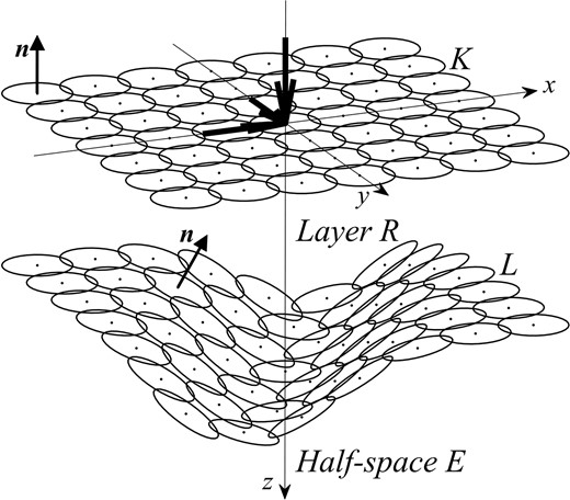
Figure 1.
3-D model of a layer R over a half-space E bounded by finite surfaces K and L. The last one is the smooth interface with half-space E. Their normal vectors n are shown. The black arrows at the origin of coordinates indicate vertical and horizontal unit harmonic loads.
The displacement field in the layer R in direction i at a point , , assuming the layer is embedded in a full space with the same properties, is given by the continuous superposition of the contributions of a force distribution on the surfaces K and L by means of force densities multiplied by surface differentials , as follows:
where is the full space Green's function with properties of layer R, it is the displacement at point in direction i for a unit harmonic force at point in direction j; and are unknown force densities at point in direction j in region R at surfaces K and L, respectively; is surface differential. Repeated sub-indices on the products within the integrands mean summation.
The traction vector in the layer R in direction i at a point at K, , is computed from the stresses by applying Hooke's law and Cauchy's surface formula, and assuming that the normal vector is upward, given by:
In the middle section of eq. (9), the first term of the equality is the contribution of force density when . It is the combined result of both derivation and integration of the singular Green's tensor of region R in the neighbourhood of the boundary (see Sánchez-Sesma & Campillo 1991). The result for the scalar case was found by Fredholm in 1900 (see Webster 1955); and the second and third terms represent the contributions of the force densities at K and L to the tractions at the surface K, and the integrals should be considered in the Cauchy principal value sense. The right end of eq. (9), is the boundary condition, represented by the product of the Kronecker and the Dirac deltas, which means a unit concentrated harmonic load at the origin, , in direction m. The index m does not appear now in the left term but has to be accounted for to give the proper meaning to the system Green's function. For tractions at region R at surface K, the first term is minus because the normal are all upward. For details see Sánchez-Sesma & Luzón (1995).
For the half-space E the displacement field is given by:
Here, is the full space Green's function, in frequency domain, with properties of region E and the force densities are acting along L. As before, the tractions at surface L are given by:
These expressions have to be discretized along the surfaces K and L for the components x, y and z corresponding to directions . We approximately discretize the domain using circles and take the centres as collocation points. This is because at the integral of the Green's tensor at each flat circle can be computed analytically and the integral of traction Green's tensor is null (for details, see Sánchez-Sesma & Luzón 1995).
Surfaces K and L are discretized and force densities are assumed constant within the element. We call and the total number of elements in K and L, respectively. The number of elements in each side of K and L are and , respectively. Therefore, and . In our implementation, and are odd numbers (typically from to ) to guarantee that the centre of our mesh is the observation point.
The tractions boundary conditions at surface K and the continuity of both tractions and displacements at L, give a system of equations that has the following structure:
where and are the centre of each of the circular surface elements in K for the observation and source points, respectively, and goes from 1 to ; and and are the centre of each of the circular surface elements in L for the observation and source points, respectively, and goes from 1 to .
The force densities in each element are assumed to be constant. They appear in the unknown vector. Therefore, the various entries in the matrix represent each a block of discretized tractions or displacements after integration in the source elements considering their centres as collocation points. For example, the block
is a matrix of by . In the term , the upper index indicates the region of validity of Green´s function (which corresponds to a full space) while the lower indices indicate: the direction of the observer's displacement and the direction of the source load; within the parentheses, the first term is the observer's collocation point and the second term is the source's collocation point.
The same applies for the force densities. For example, , we keep the first upper index to represent the region while the second upper index represents the surface of the applied sources; the term within the parentheses is the source's collocation point. Thus, the block
is a vector with the three components of force densities along surface K.
Regarding the loading points, we consider each component as an independent load vector, so we have three vectors for the loads. We assumed the load point at centre of surface K.
The solutions of eq. (12) for the three load components may allow us to compute the system Green's function. In the layer R, using the meshes K and L and a discretized version of eq. (8), we can define . The loads have the directions implicit in sub-index m. The system IMGs are calculated at the point of application of the three harmonic loads on the free-surface, the origin of the mesh, that is, .
5. ADAPTIVE MESHES
We require to evaluate the system IMGs at the source, . Then, we collect all the contributions of waves that return to such point. According to theoretical results (see Sánchez-Sesma et al. 2016), the part corresponding to the source itself is proportional to the frequency, being the instantaneous velocity, and the variations from this linear trend represent the multiples.
In low frequencies (long wavelengths), the reflections include significant amounts of non-specular waves that are precisely diffracted waves. They cancel the source up to a cut-off frequency. Therefore, non-geometric reflections may be engendered at distant points. Then, the lateral extension of the L mesh may be large to allow for the diffracted waves reaching the source point. In high frequencies (short wavelengths), the diffraction is less important, and the reflections are mainly specular and well described by rays, the clearly geometric waves require collimated reflections. Then, the lateral extent of the L mesh may be small. Fig. 2 presents a sketch of the adaptive meshes in a flat layer model.
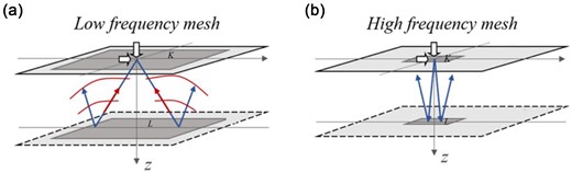
Figure 2.
3-D sketch of the adaptive meshes approach of a flat layer R over a half-space E bounded by the K mesh for the surface and the L mesh for the interface (indicated with dark grey squares): (a) for low frequencies (long wavelengths), non-geometric reflections may be engendered at distant points and the mesh extent of K and L is large; and (b) for high frequencies (short wavelengths), the reflections are specular and well described by rays and the mesh extent of K and L is small. The arrows on the surface indicate the applied loads. The light grey squares indicated the extent of the study area.
After a series of tests with small and large meshes and sundry considerations on the size of elements (uniformly located along the surface), we establish a discretization criterion: the minimum wavelength of layer R, , should be larger than eight times the radius r of the circular surface elements. Then, for the soft layer we have:
where is the shear wave propagation velocity of the layer R. Consequently, is the maximum theoretical frequency-dependent element radius and we can set where . To fulfill this condition and have a reasonable size for the minimum frequency, a horizontally isotropic geometrical scale factor, SF, is chosen to scale the mesh, which has to be applied to all horizontal dimensions and distances from the element at centre. The expression for the scale factor is:
where the first factor is less than one (here it runs from 0.75 to 0.15 in the frequency range) for fine-tuning the size of elements and the extension of the mesh. We assumed a square initial mesh K with collocation points at each side. The mesh size is then function of frequency with side .
As for the L interface mesh, its characteristics are the same if the boundary is flat. For cylindrical profile of slope or channel type the distribution of surface elements is made essentially in 2-D and the y direction follows suite. The number of elements of L may vary with frequency. For more general surfaces, good meshing is critical. However, for smooth mesh L, the surface K provides convenient support.
6. NUMERICAL RESULTS
Using the IBEM in this endeavour allows us to deal with lateral inhomogeneity at the expense of more complex calculations. This critical problem can be simplified with the development of appropriate tools to handle the geometry. Our aim is to obtain meaningful solutions that give insight into the use and limitations of the spectral ratios of ASN and their modelling using IBEM.
It is possible to have a fixed mesh which has to be computed for the maximum frequency, that is, for the shortest wavelengths, to simultaneously introduce various observation-load points and have results for all of them in the same run. This would imply having three independent load vectors and three solutions of force densities for each selected point, that is, each new observation-load point would imply three new vectors in both the independent terms and unknowns. For such a system the number of collocation points would be extremely large, scaling approximately as the square of the maximum frequency. Further scrutiny is required to assess the advantages and limitations of a fixed mesh.
Instead, we propose that our shrinking 3-D meshes scheme become local for a given observation-load point. Then, we can handle both a global and local meshes. At each observation point its local mesh shrinks as frequency grows.
This drastically reduces the computational burden if other stations have to be considered in a global array. This strategy of keeping the number of equations to solve approximately fixed, attempts to keep the problem relatively small and within the reach of diverse practitioners.
Let us describe this idea in detail. In our 3-D IBEM implementation there are two independent meshes: the global and the local. The global mesh describes the surface and the geometry of the interface. On the surface global mesh, a set of observation points are located. The local meshes are generated for each observation point and centred on it in order to calculate its response. Thus, local meshes are those to which the adaptive mesh scheme is applied and move over the global ones. At certain points such as the edges they can even exceed the latter. For the calculation at all frequencies, they have essentially the same number of points, but as the frequency increases the only point that prevails is the observation one. In fact, the separation between the collocation points decreases and then the side length of each mesh will be smaller. This frequency-dependent decrease is obtained by applying the factor (eq. 16).
In this section we present numerical results in which we model HVSR at the free-surface for three cases: (1) a single flat layer overlying a half-space; (2) a layer with a channel-like interface and (3) a layer with a smoothly varying interface making both anticlinal and synclinal shapes. These 3-D models are symmetrical with respect to the x-axis, the system Green's tensor is no longer diagonal. The current results display symmetries as well. Fortunately, the cross-term is relatively small for smooth profiles.
In the following, the local meshes K and L for the first calculation frequency of each example will be called initial mesh, and those corresponding to the last calculation frequency of each example will be called final mesh.
The physical properties of interest are the layer thickness h, the vertical and lateral extent of interface perturbation, if any, the mass density , the shear and compressional velocities of the layer R and the shear and compressional velocities of the half-space E. Two ratios are relevant to our analysis: shear velocities ratio and mass densities ratio .
6.1 Example 1
In order to illustrate our approach, we first study the case of a flat layer over a half-space. The flat surface L is at a depth m, shear wave velocities are m s−1 and m s−1, mass densities kg m−3 and kg m−3. The ratios are and . In this example, the theoretical resonance frequency of shear waves is Hz. For a flat layered medium, trustworthy reference results are available in cylindrical coordinates from the frequency–wavenumber (f-k) formulation given by Sánchez-Sesma et al. (2011b) and the improved calculation in HV-Inv software (García-Jerez et al. 2016 and Piña-Flores et al. 2017, 2024), so we can use it to calibrate our adaptive meshes for the simplest cases.
A calculation from to Hz with Hz, implies frequencies. Fig. 3(a) depicts the initial and final meshes corresponding to the first and last calculation frequencies, respectively. The K and L meshes for all frequencies have 49 elements. For each frequency, simultaneous equations are solved using the classical LU Gaussian elimination algorithm. The solution was obtained in about s (less than the analytical solution). In Fig. 3(b) the size of final surface mesh is shown. It corresponds to the frequency-dependent scaling of eq. (16). The final surface mesh occupies about one sixth of the central element of the initial surface mesh. This extraordinary behaviour shows how important in high frequencies are the strongly collimated reflections between boundary elements and the source point.
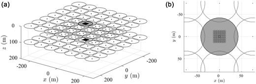
Figure 3.
3-D model of an infinite layer of thickness m and flat surface over a half-space. (a) Adaptive initial (big circles) and final (small circles) local meshes for surface K and interface L, with () collocation points each, for the observation point at the surface at m and m (grey circle). The initial mesh corresponds to the lowest frequency to be resolved, and the small one corresponds to the highest frequency of interest. (b) Detail of the final surface mesh occupying about one sixth of the central element of the initial surface mesh.
Regarding numerical results, Figs. 4(a) and (b) depict the analytical reference results for and , and HVSR, respectively. Fig. 4(a) also show the corresponding exact values for the half-space with properties of the layer in order to show how the solution include the ‘instantaneous frequency’ and clearly show a cut-off frequency produced by diffraction. On the other hand, Figs. 4(c) and (d) show the IBEM results with the adaptive meshes for and , and HVSR, respectively. A fairly good qualitative agreement is observed that shows that the physics of problem is generally accounted for. The results also highly show how well localized the solution is.
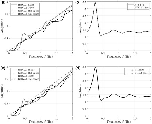
Figure 4.
HVSR of the 3-D model of a flat layer over a half-space shown in Fig. 3. (a) and (c) Imaginary parts of Green's function, and , for an observation point at the surface. (b) and (d) HVSR associated. (a) and (b) Correspond to the reference solution computed by analysis and HV-Inv which are considered as trustworthy. (c) and (d) Results from the 3-D IBEM with our adaptive meshes.
6.2 Example 2
The second example corresponds to a layer with a cylindrical channel-type interface over a half-space model. The channel looks like an inverted Gaussian. The mesh L is made along the generator in 2-D and the surface elements along the y direction are uniform following the extension of surface mesh K. Thus, the number of elements of mesh L will vary with frequency and may increase or decrease slightly. At the extremes of surface L, m and smoothly grows to a maximum depth of m; the variation along x-axis (for m) is given by two cubics. Along y-axis the depths are constant. The shear wave velocities are m s−1 and m s−1, mass densities kg m−3 and kg m−3. The ratios are and .
Fig. 5(a) depicts the initial and final meshes K and L for the observation point at the origin coinciding with the centre of interface topography. Mesh K is flat and conserves elements (), while mesh L have elements (). The two initial meshes (for Hz) cover approximately a horizontal surface of about m2 while the last meshes (for Hz) cover only m2. The mesh size reduction is gradual, at the end the linear dimension of mesh is (regarding the area, it is ) but the number of equations remains practically constant. Slightly larger meshes were used and results do not present changes suggesting that the contributions of layer-associated boundary sources are well represented by the used meshes, which are constructed for each frequency. We found that closely collimated reflections are essential in high frequencies and wide reflection angles still generate energy contributions at the source for low frequencies. This is the subject of our current research.
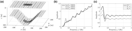
Figure 5.
3-D model of an infinite layer with a flat surface over a half-space with a cylindrical channel-type interface. The layer thickness varies from m for m, reaching m at the centre. (a) Adaptive initial (big circles) and final (small circles) local meshes for surface K and interface L, for the observation point at the surface at m and m (grey circle); (b) IBEM results for imaginary parts of Green's function of the system, , and for the observation point of (a); and (c) total and directional-HVSR: and , for the same point.
The theoretical frequency of a uniform layer of thickness m is Hz. The numerical calculations give a value of Hz and significant difference in horizontal directions. The single components are and , and the total HVSR is . For this observation point, the maximum value of HVSR is along y-axis, almost two times the value along x-axis. This suggests enhanced waves along y-axis and/or large stiffness along x-axis. This channel-like model resembles the configuration studied by Matsushima et al. (2017) for Onahama, Tohoku, Japan, and the results qualitatively agree. There is a significant increase in HVSR in the direction of channel. For various positions of the observation point along x-axis (not shown here), the behaviour of HVSR changes. At the top of the edge, the components are similar and for values of m the component along x-axis is larger, for m the symmetry is recovered.
Fig. 5(b) displays some peaks in higher frequencies that reveal trapped waves that we are currently studying. It is of interest at this point to display the azimuthal variation of results. This variation is already shown in Fig. 5(c), but a more suggestive description can be achieved projecting the results according to eq. (7).
The contours of the are displayed in Fig. 6. The symmetry and the strong directionality are evident. This type of display has to be studied in detail as it can be retrieved from field data. It is a challenge to unlock most of the causative factors which are in a shadow so far.
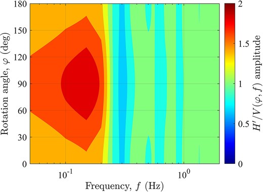
Figure 6.
Contour plots of directional HVSR ( of a layer with a deep channel-like interface model shown in Fig. 5(a), at the surface observation point located at m and m, for frequencies up to Hz and . The contours show a peak of about at Hz for , the direction of the cylinder, and have a minimum at (and ), recovering amplitude at Hz.
6.3 Example 3
The third example corresponds to an infinite layer with a flat surface over a half-space with an interface formed by a syncline-shape and an anticlinal-shape. This analytical shape is given by , where . Now the variables x, y and h are dimensionless and in what follows are scaled by a common dimension factor ( m, which is the depth of the flat reference layer). The shear wave velocities are m s−1 and m s−1, mass densities kg m−3 and kg m−3. The ratios are and . The dominance frequency of the flat reference layer is Hz.
Fig. 7(a) shows the global mesh of the interface geometry; the syncline shape is centred at m and m with thicknesses m, and the anticlinal shape is centred at m and m with thicknesses m. Fig. 7(b) shows the surface global mesh where observation points are regularly distributed over a square of 9 points on each side. To obtain the HVSR at these observation points, local meshes are generated, centred at each point, whose collocation points in this particular case are for the L mesh () and for the K mesh (). A schematic example is shown in Fig. 7(b) for point , for which the local mesh K used to calculate its response is indicated by a red line. Note that the red square exceeds the boundaries of the global mesh, where the observers are located but the interface is well defined everywhere. Surface L is discretized starting with the horizontal positions of mesh K and iterative corrections in each direction are performed to improve the representation of interface with a uniform distribution of the circular elements along the surface. This simple model configuration captures some spatial variation that can be found in reality.
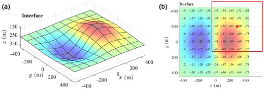
Figure 7.
3-D model of an infinite layer with a flat surface over a half-space with an interface formed by a syncline-shape and an anticlinal-shape. (a) Global mesh of the interface; the syncline-shape is centred at m and m with thicknesses m. The anticlinal-shape is centred at m and m with thicknesses m. (b) Global mesh of the surface where the observation points are marked and numbered. As a schematic example, the local mesh K used to calculate the response for point 70 (marked with a circle) is indicated by a bulk line.
In a relatively straightforward manner, the results are obtained for all global mesh points in about a minute for each one using a common laptop.
In Figs 8(a), (c) and (d) display the results for an observation point located above the topography L at the maximum thickness m (at m and m) forming a kind of valley. The frequency corresponding to a flat layer with m is Hz while the computed peak is about Hz (Fig. 8d). The IMGs in Fig. 8(c) display significant peaks in the horizontal components that suggest trapping of shear waves and local mode resonances (see Rial et al. 1992). However, have a small amplitude.
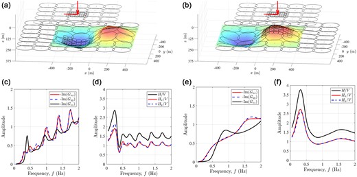
Figure 8.
HVSR for the 3-D model of an infinite layer with a flat surface over a half-space with an interface formed by a syncline-shape and an anticlinal-shape shown in Fig. 7. (a) Adaptive initial (big circles) and final (small circles) local meshes for surface K and interface L, for the observation point at the surface at m and m (point 23 in Fig. 7b), colourmap indicate the global mesh for the interface; (b) adaptive initial (big circles) and final (small circles) local meshes for surface K and interface L, for the observation point at the surface at m and m (point 59 in Fig. 7b), colourmap indicate the global mesh for the interface; (c) and (d) imaginary parts of Green´s function, and total and directional-HVSR: and , respectively, for the observation point at (a), (c) and (d) imaginary parts of Green´s function, and total and directional-HVSR: and , respectively, for the observation point at (b).
Figs 8(b), (e) and (f) display the results for a surface observation point (at m and m), above the top of the topography of profile L with the minimum thickness m. The frequency corresponding to a flat layer with m is Hz while the computed peak is about Hz (Fig. 8f). Both the IMGs and the are rather smooth (see Figs 8e and f, respectively). In higher frequencies, this site above the underground hill shows that a good part of the energy seems to be scattered away and has a smooth shape. This behaviour of in a convex setting may be useful to explain the absence of local resonances or, in other words, of local modes, as suggested by Rial et al. (1992).
As in the channel-like example in this anticlinal–synclinal shape somehow larger meshes were employed and results are stable. The HVSR results depend on the position of the observer. The simplicity of the horizontally layered case is lost. Now we have positional and directional effects. For the ‘bump’ anticlinal shape of Fig. 8(b) the has large amplitudes and smooth shapes suggesting that the emitted waves are scattered away by the geometrical configuration (see Figs 8e and f), while for the ‘pouch’ of Fig. 8(a) the peak is small with rough behaviour (Figs 8c and d) associated to energy trapping; the emergence of peaks suggests local modes. These may produce damage in seismic events where large amount of energy is supplied into the system. Closely collimated reflections give significant contributions to the energy budget in high frequencies while wide reflection angles give energy contributions at the source for low frequencies.
Fig. 9 displays the spatial location of peak amplitude values and associated frequencies for the observation points in the horizontal domain displayed in Fig. 7. As expected, both distributions show an asymmetrical behaviour along x-axis.
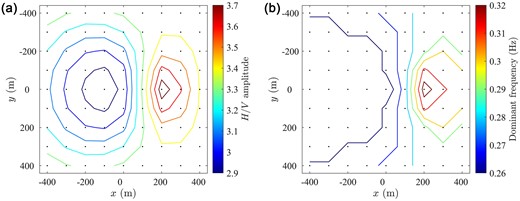
Figure 9.
HVSR main peak contours of (a) amplitude and (b) fundamental frequency of the -station array of the 3-D model of an infinite layer with a flat surface over a half-space with an interface formed by a syncline-shape and an anticline-shape shown in Fig. 7.
In this example, there are points in which the directional-HVSR was obtained. Adapting Matsushima et al. (2017) directionally dependent coefficient (), we use the following expression,
This directional measure averages in the frequency range between and for which we have N samples. allows us to classify the sites according to their directional dependence. In this expression, indicates almost no lateral inhomogeneity for the selected frequency range, being f the central value which may provide a clue for origin depth of the directionality. An adequate modelling strategy for inversion has yet to be developed.
Fig. 10 displays at the points the vectors whose direction is governed by the rotation angle of the directional-HVSR at which the maximum values of are found, the modulus of the vectors is the value of . Comparing the vectors of the maximum of the stations array (Fig. 10) with the geometry of the interface (Fig. 7), in the anticline area (right side), the direction of the vectors seems to surround the irregularity, with a minimum value of the module found at the top of it. In the synclinal zone (left side) the direction of the vectors is parallel, and it is seen as if they entered the irregularity. The minimum values of the modules are found when areas that resemble flat layers are found, as is the case of the stations located at m. The vectors in Fig. 10 convey the idea of a fundamental local mode and the flow of energy suggests a torsional behaviour. Other local modes can be spotted at higher frequencies and are subjects of our current research.
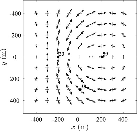
Figure 10.
Direction and modulus of the maximum directionally dependent coefficient () of the -stations array of the 3-D model of an infinite layer with a flat surface over a half-space with an interface formed by a syncline-shape and an anticline-shape shown in Fig. 7 for the frequency Hz. Three stations marked with a dot and numbered are selected to show the directional-HVSR () in Fig. 11 (see Fig. 7b for station reference).
Three stations 23, 38 and 59 (Fig. 10) were selected to display the directional-HVSR against azimuth and frequency, and the corresponding to the azimuths for the maximum at the peak frequencies. Fig. 11 displays these results.
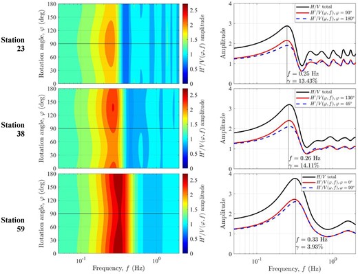
Figure 11.
Directional-HVSR () for three stations of the 3-D model of an infinite layer with a flat surface over a half-space with an interface formed by a syncline-shape and an anticline-shape shown in Fig. 7, in the left column. Total and corresponding to the maximum directionally dependent coefficient () obtained from the directional-HVSRs in the right column (see Fig. 7b for station reference).
Station 23 is at the centre of the synclinal zone; the module at the peak frequency suggests the presence of an irregularity. Station 59 is at the centre of the anticlinal zone; at the peak frequency the module is small as in the flat layer case. Station 38 is located over the slope of the anticline zone; at the peak frequency, module has one of the maximum values found in the array suggesting a lateral change. Indeed, its direction is parallel to the contours of the irregularity. These results suggest the importance of measurements using dense arrays that can contribute to making a trustworthy interpretation.
7. OBSERVED DIRECTIONAL-HVSR AT CHALCO, VALLEY OF MEXICO
At the southern part of the Valley of Mexico, in the Chalco region were used to be a lake (Fig. 12). ASN measurements ( min of recording) at sites were analysed to obtain HVSRs and directional-HVSRs (Baena-Rivera et al. 2024). Fig. 12 shows the deployment of the Chalco array that covered approximately km2, with a maximum distance between points of m, and a minimum of m.
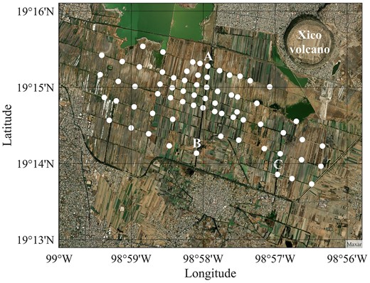
Figure 12.
Satellite image with location of the Chalco array at the southern part of the Valley of Mexico (Mapping Toolbox—MATLAB), with the measured points georeferenced in white. Stations marked with A, B and C were selected for discussion in Section 7.
The total and the directional-HVSR () at three sites of the Chalco array (see Fig. 12) are displayed in Fig. 13. The total and small at the peak frequency allowed to make a reliable standard inversion for station A. In contrast, at stations B and C, the directional-HVSR () suggests significant effects of lateral variations.
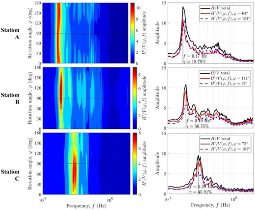
Figure 13.
Measurements of directional-HVSR at three sites in Chalco array, Valley of Mexico. Left column, directional-HVSR,, for three stations. Right column, total and the minimum and maximum values for each station.
Station A shows a minimum value at Hz (see Fig. 13), which indicates an area where the energy propagates as in the case of flat layers, so it is assumed to be an area with low irregularity. Stations B and C present significant values at Hz and Hz, respectively, which a priori indicates areas with significant lateral variations. Since there are no nearby stations, it is not possible to map or determine the nature of the detected disturbance. Further discussions can be found in Baena-Rivera et al. (2024).
8. CONCLUSIONS
For a single layer with varying interface, we model the system IMGs using 3-D IBEM. This approach allows the analyst to use the principle of superposition and construct the fields as summations of contributions of unknown force densities, after fulfillment of boundary conditions. This model allowed us to point out the complexity of the problem and opens the door to the numerical modelling based on the diffuse field assumption. Certainly, the exercise could be facilitated if trustworthy information of the system configuration is available (e.g. Matsushima et al. 2017; Perton et al. 2017). The numerical solution of 3-D realistic cases can be very demanding of computer resources. In the design of our simple one-layer model with smooth varying interface, we tried to keep the problem with a reasonable small size and devise adaptive meshes that change size with frequency. Our strategy is based on the properties of diffracted waves which display distinct behaviour at low and high frequencies. This is based upon our preferred interpretation of the cut-off frequencies that appear in the system IMGs spectra. We tested the adaptive mesh concept for the flat layer case with reasonable qualitative results. The concept of locality employed in the modelling can be extended along the lines of reasoning pioneered more than three decades ago by Rial et al. (1992) using local modes and by Kanai (1983) at the beginning of the 20th century.
For a layer over a half-space with a laterally varying interface, we obtained the directional-HVSR detecting both changes in peak frequency and amplitudes for varying azimuth. From these results, it is far from realistic to invert the total HVSR to estimate the vertical velocity model using flat layers.
The full directional-HVSR reveals a more complex problem like the opening of Pandora's box. Fortunately, the 3-D IBEM is a powerful method formulated in the frequency domain. The SEM has also been used for modelling HVSR with success for a known configuration (Matsushima et al. 2017). Here we focused on smooth interface variations and the results are consistent but require further scrutiny to clarify the advantages and limitations of the technique and the simplifications we propose herein. We believe it is too early to foresee the inversion of the structure using one or a few measuring points. The potential variations of possible substructures greatly exceed any information present in a single HVSR measurement. Recorded data in Chalco, at the southern part of the Valley of Mexico, reinforces this idea (Baena-Rivera et al. 2024). One must supplement measurements with extra geophysical information, possibly non-seismic.
A growing number of tasks emerges. A new set of approaches, such as gathering data from dense arrays of measurements, more complete parametric analysis and new ideas to interpret polarizations are needed to generate practical recommendations. The calculation of pseudo-reflection seismograms (PRS) as discussed in Scherbaum (1987) and Sánchez-Sesma et al. (2016) is a pending task. The PRS and the polarization results in the directional-HVSR could be useful to establish the nature of local modes. The measurements themselves have to be used extensively as an output of an analogue computer to foresee possible responses in case of earthquakes.
Acknowledgements
Many thanks are given to R. Avila-Carrera, M. Campillo, E. de Mejía, J.G. González, L.F. Kallivokas, O.I. López-Sugahara, J.C. Pardo-Dañino, J. H. Spurlin, F. Storey and L. Rivera for their comments and suggestions. Particular thanks to I.R. Valverde-Guerrero for his multifarious help. C. Carreón-Otañez participated in early stages of this research. The careful and insightful reviews of S. Matsushima, Y. Zheng and H. Chauris contributed to greatly improve the manuscript. J.E. Plata and M.G. Sánchez of USI-IINGEN, UNAM (Universidad Nacional Autónoma de México), helped locating useful references. This work was partially supported by the UNAM-University of Illinois Research Partnership Program 2023 and by UNAM's DGAPA (Dirección General de Asuntos del Personal Académico) under projects PAPIIT IN105523 and IN104823.
Author contributions: FJS-S and RLW conceived the study and drew the general layout, interpreted the results and wrote the manuscript. MB-R, MP, DAR-Z and FJS-S wrote the codes and performed numerical computations. AA-C organized Chalco, Valley of Mexico, experiment collected the seismograms and interpreted results. MB-R and AA-C analysed the Chalco data, made the numerical models and computed the directional-HVSR and polarization information. MB-R and DAR-Z generated numerical meshes. All authors contributed with discussions and improvements of the manuscript.
DATA AVAILABILITY
The seismograms used in this study were collected by AA-C. Data are available upon request to the corresponding author. The synthetic seismograms used in this study were computed by means of computer codes wrote by the authors and are available upon request to FJS-S.
References
Aki
K.
,
1957
.
Space and time spectra of stationary stochastic waves with special reference to microtremors
,
Bull. Earthq. Res. Inst.
,
35
,
415
–
456
.. Available at:
Arai
H.
,
Tokimatsu
K.
,
2004
.
S-wave velocity profiling by inversion of microtremor H/V spectrum
,
Bull. seism. Soc. Am.
,
94
,
53
–
63
..
Baena-Rivera
M.
,
Arciniega-Ceballos
A.
,
Sánchez-Sesma
F.J.
,
Rosado-Fuentes
A.
,
Pardo-Dañino
J.C.
,
2024
.
Directional HVSR at the Chalco lakebed zone of the Valley of Mexico: analysis and interpretation
,
J. Appl. Geophys.
,
228
,
105452
,
Campillo
M.
,
Paul
A.
,
2003
.
Long range correlations in the seismic coda
,
Science
,
299
,
547
–
549
..
European Research Project
S.E.S.A.M.E.
,
2004
.
Guidelines for the implementation of the H/V spectral ratio technique on ambient vibrations measurements
,
Processing and Interpretation. European Commission—Research General Directorate
. .
García-Jerez
A.
,
Piña-Flores
J.
,
Sánchez-Sesma
F.J.
,
Luzón
F.
,
Perton
M.
,
2016
.
A computer code for forward computation and inversion of the H/V spectral ratio under the diffuse field assumption
,
Comput. Geosci.
,
97
,
67
–
78
..
Hennino
R.
,
Tregoures
N.
,
Shapiro
N.
,
Margerin
L.
,
Campillo
M.
,
van Tiggelen
B.
,
Weaver
R.L.
,
2001
.
Observation of equipartition of seismic waves in Mexico
,
Phys. Rev. Lett.
,
86
,
3447
–
3450
..
Kanai
K.
,
1983
.
Engineering Seismology
,
251p
.,
University of Tokyo Press
.
Lontsi
A.M.
et al.
2019
.
A generalized theory for full microtremor horizontal-to-vertical [H/V (z, f)] spectral ratio interpretation in offshore and onshore environments
,
Geophys. J. Int.
,
218
,
1276
–
1297
..
Lontsi
A.M.
,
Sánchez-Sesma
F.J.
,
Molina-Villegas
J.C.
,
Ohrnberger
M.
,
Krüger
F.
,
2015
.
Full microtremor H/V (z, f) inversion for shallow subsurface characterization
,
Geophys. J. Int.
,
202
(
1
),
298
–
312
..
Matsushima
S.
,
Hirokawa
T.
,
de Martin
F.
,
Kawase
H.
,
Sánchez-Sesma
F.J.
,
2014
.
The effect of lateral heterogeneity on horizontal-to-vertical spectral ratio of microtremors inferred from observation and synthetics
,
Bull. seism. Soc. Am.
,
104
,
381
–
393
..
Matsushima
S.
,
Kosaka
H.
,
Kawase
H.
,
2017
.
Directionally dependent horizontal-to-vertical spectral ratios of microtremors at Onahama, Fukushima, Japan
,
Earth Planets Space
,
69
,
96
.
Miller
G.F.
,
Pursey
H.
,
1955
.
On the partition of energy between elastic waves in a semi-infinite solid
,
Proc. R. Soc. Lond. Series A, Mathematical and Physical Sciences
,
233
,
55
–
69
.. doi:
Molnar
S.
et al.
2022
.
A review of the microtremor horizontal-to-vertical spectral ratio (MHVSR) method
,
J. Seismol.
,
26
,
653
–
685
..
Nakamura
Y.
,
1989
.
A method for dynamic characteristics estimation of subsurface using microtremor on ground surface
,
Q. Rep. RTRI
,
30
,
25
–
33
.
Nogoshi
M.
,
Igarashi
T.
,
1971
.
On the amplitude characteristics of microtremor (part 2)
,
J. Seismol. Soc. Japan
,
24
,
26
–
40
.. doi:
Perton
M.
,
Sánchez-Sesma
F.J.
,
2015
.
The indirect boundary element method to simulate elastic wave propagation in a 2-D piecewise homogeneous domain
,
Geophys. J. Int.
,
202
,
1760
–
1769
..
Perton
M.
,
Sánchez-Sesma
F.J.
,
Rodríguez-Castellanos
A.
,
Campillo
M.
,
Weaver
R.L.
,
2009
.
Two perspectives on equipartition in diffuse elastic fields in three dimensions
,
J. acoust. Soc. Am.
,
126
,
1125
–
1113
..
Perton
M.
,
Spica
Z.
,
Caudron
C.
,
2017
.
Inversion of the horizontal to vertical spectral ratio in presence of strong lateral heterogeneity
,
Geophys. J. Int.
,
212
(
2
),
930
–
941
..
Piña-Flores
J.
,
Cárdenas-Soto
M.
,
García-Jerez
A.
,
Campillo
M.
,
Sánchez-Sesma
F.J.
,
2021
.
The search of diffusive properties in ambient seismic noise
,
Bull. seism. Soc. Am.
,
111
,
1650
–
1660
..
Piña-Flores
J.
,
García-Jerez
A.
,
Sánchez-Sesma
F.J.
,
Luzón
F.
,
Márquez-Domínguez
S.
,
2024
.
HV-Inv: a MATLAB-based graphical tool for the direct and inverse problems of the horizontal-to-vertical spectral ratio under the diffuse field theory
,
Softw. Impacts
,
22
,
100706
.
Piña-Flores
J.
,
Perton
M.
,
García-Jerez
A.
,
Carmona
E.
,
Luzón
F.
,
Molina-Villegas
J.C.
,
Sánchez-Sesma
F.J.
,
2017
.
The inversion of spectral ratio H/V in a layered system using the diffuse field assumption (DFA)
,
Geophys. J. Int.
,
208
(
1
),
577
–
588
..
Pischiutta
M.
,
Fondriest
M.
,
Demurtas
M.
,
Di Toro
G.
,
Magnoni
F.
,
Rovelli
A.
,
2017
.
Structural control on the directional amplification of seismic noise (Campo Imperatore, central Italy)
,
Earth Planet. Sci. Lett.
,
471
,
10
–
18
..
Sánchez-Sesma
F.J.
,
Campillo
M.
,
1991
.
Diffraction of P, SV, and Rayleigh waves by topographic features: a boundary integral formulation
,
Bull. seism. Soc. Am.
,
81
(
6
),
2234
–
2253
.. doi:
Sánchez-Sesma
F.J.
,
Campillo
M.
,
2006
.
Retrieval of the Green's function from cross-correlation: the canonical elastic problem
,
Bull. seism. Soc. Am.
,
96
(
3
),
1182
–
1191
..
Sánchez-Sesma
F.J.
,
Luzón
F.
,
1995
.
Seismic response of three-dimensional alluvial valleys for incident P, S, and Rayleigh Waves
,
Bull. seism. Soc. Am.
,
85
(
1
),
269
–
284
.. doi:
Sánchez-Sesma
F.J.
et al.
2011b
.
A theory for microtremor H/V spectral ratio: application for a layered medium
,
Geophys. J. Int.
,
186
(
1
),
221
–
225
..
Sánchez-Sesma
F.J.
,
2017
.
Modeling and inversion of the microtremor H/V spectral ratio: physical basis behind the diffuse field approach
,
Earth Planets Space
,
69
,
92
. doi:
Sánchez-Sesma
F.J.
,
Iturrarán-Viveros
U.
,
Perton
M.
,
2016
.
Some properties of Green's functions for diffuse field interpretation
,
Math. Methods Appl. Sci.
,
40
(
9
),
3348
–
3354
..
Sánchez-Sesma
F.J.
,
Pérez-Ruiz
J.A.
,
Luzón
F.
,
Campillo
M.
,
Rodríguez-Castellanos
A.
,
2008
.
Diffuse fields in dynamic elasticity
,
Wave Motion
,
45
,
641
–
654
..
Sánchez-Sesma
F.J.
,
Weaver
R.L.
,
Kawase
H.
,
Matsushima
S.
,
Luzón
F.
,
Campillo
M.
,
2011a
.
Energy partitions among elastic waves for dynamic surface loads in a semi-infinite solid
,
Bull. seism. Soc. Am.
,
101
(
4
),
1704
–
1709
..
Scherbaum
F.
,
1987
.
Seismic imaging of the site response using microearthquake recordings. Part II. Application to the Swabian Jura, Southwest Germany, seismic network
,
Bull seism. Soc. Am.
,
77
(
6
),
1924
–
1944
..
Schuster
G.T.
,
2009
.
Seismic Interferometry
,
Cambridge Univ. Press
.
Shapiro
N. M.
,
Campillo
M.
,
Stehly
L.
,
Ritzwoller
M.
,
2005
.
High resolution surface wave tomography from ambient seismic noise
,
Science
,
307
,
1615
–
1618
.
Stokes
G.G.
,
1849
.
On the dynamic theory of diffraction
,
Trans. Camb. Philos. Soc.
,
9
,
1
–
62
.
Weaver
R.L.
,
Lobkis
O.I.
,
2001
.
Ultrasonics without a source. Thermal fluctuation correlations at MHz frequencies
,
Phys. Rev. Lett.
,
87
,
134301
.
Weaver
R.L.
,
Yoritomo
J.Y.
,
2018
.
Temporally weighting a time varying noise field to improve green function retrieval
,
J. acoust. Soc. Am.
,
143
(
6
),
3706
–
3719
..
Weaver
R.L.
,
1982
.
On diffuse waves in solid media
,
J. acoust. Soc. Am.
,
71
,
1608
–
1609
..
Weaver
R.L.
,
1985
.
Diffuse elastic waves at a free surface
,
J. acoust. Soc. Am.
,
78
,
131
–
136
..
Webster
A.G.
,
1955
.
Partial Differential Equations in Mathematical Physics
,
Dover
.
APPENDIX. GREEN'S FUNCTION FOR A FULL SPACE
For the sake of completeness, we give here the expression of the Green's function (see Stokes 1849; Sánchez-Sesma & Luzón 1995) in an unbounded space E:
where is the distance between , are the direction cosines of the source–receiver unit vector ; is shear modulus, is mass density, is shear wave velocity, is compressional wave velocity. The functions and are given in term of the shear and compressional wave numbers and , by means of
and
which have the constants 1 and (1 + )/2, respectively, as limits if or r tends to zero.
The corresponding Green's tractions are given by,
Further details can be found in Sánchez-Sesma & Luzón (1995).
© The Author(s) 2025. Published by Oxford University Press on behalf of The Royal Astronomical Society.
This is an Open Access article distributed under the terms of the Creative Commons Attribution License (
https://creativecommons.org/licenses/by/4.0/), which permits unrestricted reuse, distribution, and reproduction in any medium, provided the original work is properly cited.


