


SUMMARY
Utilizing statistical tests to evaluate earthquake forecasting models is crucial to improve forecasting strategies for seismic hazard assessment. We develop a novel evaluation method for alarm-based earthquake forecast, taking into account the magnitude of seismic energy and the impact area of earthquakes, instead of using solely seismic event number and epicentre locations in conventional approaches. First, we derive a scale law of Seismic Area by statistically analysing coseismal maps of past M ≥ 7.0 earthquakes. Second, we proportionally allocate Seismic Moment to surrounding cells based on corresponding seismic area within each cell (SASM-test). Compared to the Molchan test which is conventionally applied for models that forecast the epicentre location, our proposed SASM-test can be applied to the evaluation of forecasting models that focus on the whole earthquake rupture (source area). Third, we apply the SASM-test method to the time-independent probabilistic earthquake forecasting model for the southeastern Tibetan Plateau (RELM-TibetSE) and compare it with other evaluation methods. The retrospective testing shows that the SASM-test demonstrate relatively higher sensitivity, enabling to detect subtle differences between similar models that conventional methods may overlook. Additionally, retrospective test results indicate that: (i) Earthquake forecasting models using Global Navigation Satellite System (GNSS) data performed better in forecasting the ‘source area’ than the ‘epicentre location’; (ii) forecasting models based on principal strain rate outperformed the models based on maximum shear strain rate in forecasting both the epicentre location and the source area and (iii) incorporating spatially varying seismogenic layer thickness and rigidity into seismic forecasting models could improve their ability to forecast the ‘source area’ compared to using uniform seismogenic layer properties. The newly proposed SASM-test method can provide a more sensitive and comprehensive approach for the evaluation of earthquake forecasting models, contributing to the refinement of seismic hazard assessments.
1 INTRODUCTION
A statistically effective earthquake forecasting model is crucial to seismic hazard assessment. Numerous Regional Earthquake Likelihood Models (RELM) are proposed to improve disaster preparedness over past decades for earthquake-prone regions, such as California (Bird & Liu 2007; Field et al. 2007, 2009, 2014, 2015, 2017; Rhoades 2007; Shen et al. 2007; Zeng et al. 2018; Rollins & Avouac 2019) and Southeastern Tibet (Wang et al. 2015; Wang et al. 2019; Cheng et al. 2020; Li et al. 2023; Wei et al. 2023). A key question arises from the various RELMs: which model is more trustworthy? To answer this question, Southern California Earthquake Center conducted likelihood consistency tests to evaluate the agreement of forecasting models with actual seismic activity (Jordan 2006) using various evaluation methods, including Number test (Kagan & Jackson 1995; Schorlemmer et al. 2007), Likelihood test (Moschetti et al. 2016) and Molchan error diagram (Molchan-test; Molchan 1990, 1991, 1997, 2010; Molchan & Kagan 1992; Wang et al. 2013). Additionally, statistical tests, such as information gain per earthquake (IGPE, Imoto 2007; Nandan et al. 2019) and T-test (Rhoades et al. 2011) can be employed to assess earthquake likelihood models.
Molchan-test enable to assess the forecasting efficacy of various earthquake likelihood models at different alarm thresholds, and further to refine the seismic forecasting models. Molchan-test require spatially discretized forecasting indicators, projecting epicentres onto each grid cell, and calculating miss rates at various alarm thresholds. Molchan-test is widely applied in testing earthquake forecasting models. For instance, Rhoades et al. (2017) tested a multiplicative hybrid earthquake likelihood model in New Zealand. Talbi et al. (2013) retrospectively tested a new earthquake forecasting model in Japan, employing the moment ratio of the first- to second-order moments of earthquake interevent times as a precursory alarm index for forecasting large seismic events. Xiong et al. (2021) used the Molchan-test to examine the correlation between strain rate fields and seismic activity in China. However, it might be overly simplistic to calculate miss rate solely based on ‘proportion of unforecasted earthquakes relative to total earthquakes’. As earthquake impact is beyond a single point at the epicentre, it usually involves rock volume sliding. Thus, a forecasting model should forecast not only epicentre locations but also the magnitude and range of seismic energy release. Accordingly, the method using only epicentre locations might be less effective than the one with earthquake impact zone considered in evaluating forecasting models.
In this study, we develop a novel method for evaluating earthquake forecasting models, known as the SASM-test, taking into account earthquake magnitude and impact area, rather than the number of seismic events and epicentre locations. We first conduct statistical analysis of seismic intensity maps and derive a scaling law for the ratio of the major to minor axes of the seismic area. We then allocate the seismic moment to assess model forecasting performance. Additionally, we apply the SASM-test method to the time-independent probabilistic earthquake forecasting model of the southeastern Tibetan Plateau (RELM-TibetSE) and compare the SASM-test method with other evaluation methods, providing detailed analyses of the advantage and disadvantage of each testing method. Finally, we compare the retrospective testing results of six submodels of the RELM-TibetSE. The comparison of test results could provide significant guidance for the selection of GNSS strain rates and seismogenic layer structures in the future development of earthquake forecast models. The newly proposed method is characterized by a more accurate assessment of the reliability of seismic forecasting models, which is conducive to the mitigation of seismic hazards.
2 SEISMIC MOMENT ALLOCATION FOR VERIFYING EARTHQUAKE FORECASTING MODEL
2.1 Methodology
If the RELM provides spatial forecasting indices (alarm), Molchan-test can evaluate its performance by defining the relationship between proportion of space occupied by the alarm (τ) and miss rate (υn) using Molchan error diagrams. Figs 1(a) and (b) show principles of Molchan-test and our proposed SASM-test. The Molchan-test discretize forecasting indices spatially and projecting epicentre locations onto the discretized grid. Epicentre in alerted cells (shaded in Fig. 1a) count as hit (successful forecast), while other cells are as miss (unsuccessful forecast). The threshold is lowered until all targeted earthquakes are correctly forecasted.
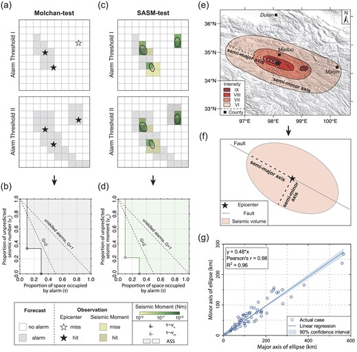
Schematic diagrams of the principles for Molchan-test and our proposed SASM-test. (a) Molchan-test alarms under different thresholds in spatial discretization of alarm functions. Stars represent the epicentre; (b) Molchan error diagram and (c) SASM-test alarms under different thresholds in spatial discretization of alarm functions. Ellipses represent the seismic area; (d) SASM error diagram and (e) seismic intensity map of the 2021 Ms 7.4 Maduo earthquake, northeastern Tibetan Plateau, China. The coseismal contours on a horizontal surface plane were obtained from the China Earthquake Administration (CEA) available at www.mem.gov.cn/xw/yjglbgzdt/202105/t20210528_386251.shtml; (f) schematic diagram of the elliptical model of earthquake area and (g) linear regression analysis of the major and minor axes of the elliptical model of large earthquakes from BC 70 to AD 2021 over Chinese continent, as listed in Table S1 (Supporting Information).
An earthquake epicentre provides the nucleation locus of its source rupture, which cannot reflect impact range of the event itself. Therefore, to verify the forecasting ability of an earthquake forecasting model, we need also to take in account the magnitude and impact range of earthquakes, in addition to the number and epicentre positions. As the magnitude of an earthquake can be described by its seismic moment, we define the primary impact range of an earthquake on the Earth's surface as its seismic area.
In the SASM-test method, we allocate seismic moment to surrounding cells based on the proportionality between the area of seismic area within the cell and the seismic moment assigned to each cell, substituting the epicentre distribution in Molchan-test (Fig. 1a) with the seismic moment distribution (Fig. 1c). Thus, in the SASM-test, ‘hit’ refers to correctly capturing the distribution of seismic moment, rather than accurately forecasting the epicentre location. In SASM-test error diagram (Fig. 1d), we calculate seismic moment miss rate (|${{\upsilon }_m}$|) as the ratio of unforecasted seismic moment that fails to meet a specific forecast threshold to total seismic moment (eq. ). The proportion of space occupied by the alarm (τ) can be expressed by eq. (2):
where, |$P( i )$| represents the forecasting indicator value for the ith cell, such as the earthquake forecast probability in the ith cell in the RELM. |$plevel$| is the threshold for the forecasting indicator values; |${{M}_o}( i )$| denotes the seismic moment value within the ith alerted cell and |$A( i )$| is the area of the ith cell. The τ and ν range from 0 to 1.
When applying SASM-test to evaluate forecasting models, we first collect seismic catalogue of study area, and then calculate seismic moment from the seismicity. Next, the seismic moment of each earthquake is allocated to the spatially discretized cells based on its seismic area. For instance, as shown in Fig. 1(c), the coloured cells display the distributed seismic moment. Finally, by progressively lowering the threshold of alarm, we calculate the proportion of space–time occupied by the alarm (τ) and the corresponding seismic moment miss rate (|${{\upsilon }_m}$|), and then plot the (τ,|${{\upsilon }_m}$|) step curve on the SASM-test error diagram (Fig. 1d).
The forecasting performance can be evaluated in several ways: (1) estimating probability gain (G) from SASM-test error diagram. Molchan (1991) provided a method to calculate G in eq. (3). If the (τ, |${{\upsilon }_m}$|) step curve falls below and to the left of dashed line at G = 1, it indicates the model performs better than random forecasting. A higher G signifies better forecasting performance. (2) Assessing the distance between the (τ, |${{\upsilon }_m}$|) curve and the horizontal and vertical coordinate axes. For model with better forecasting performance, the (τ, |${{\upsilon }_m}$|) curve is closer to the Y- and X-axes. (3) Estimating area skill score (ASS). The ASS uses the Molchan diagram particularly for continuous alarm functions (Zechar & Jordan 2008). Specifically, the area enclosed by the (τ, |${{\upsilon }_m}$|) curve, τ = 1 and |${{\upsilon }_m}$|=1 lines is known as ASS. A larger ASS indicates a better forecasting and that earthquakes are concentrated in cells with higher forecasted probabilities. (4) Assessing forecast capacity by the proportion of seismic moment forecasted within the top 30 per cent high-probability cells. A higher proportion indicates greater forecasting ability. (5) Examine the relationship between each point on the (τ, |${{\upsilon }_m}$|) curve and the significance level (|${\rm{\alpha }}$|) contour lines corresponding to the number of ‘hit’. The distribution probability that h or more events are ‘hit’ (i.e. forecasted) out of a total of N events can be represented by the binomial expression eq. (4). The corresponding significance level (|${\rm{\alpha }}$|) can be calculated using eq. (5)
where, |$N$| represents the total number of earthquakes, and |$h$| denotes the number of earthquakes that have been ‘hit’ (i.e. successfully forecasted).
2.2 Seismic area and the allocation of seismic moment
Given unavailability of source rupture models for certain historical earthquakes, the SASM-test method allocates moment of each earthquake to surrounding cells proportionally to the earthquake area in each cell. Here, seismic area is defined as the zone of perceived intensity and surface destruction of an earthquake. Seismic intensity map, which reflects the distribution of earthquake energy at the surface, corresponds well to the seismic area as defined in the proposed SASM-test method, enabling the estimation of seismic area accordingly.
However, intensity distributions vary among different earthquakes. An elliptical model is conventionally employed to describe earthquake intensity distributions (Chen & Liu 1989). For instance, the intensity map of the 2021 Ms 7.4 Maduo earthquake, northeastern Tibetan Plateau, China (Fig. 1e) shows clearly elliptical coseismal contours on a horizontal surface plane. Therefore, we adopt an elliptical model to represent seismic area distribution (Fig. 1f).
The geometric centre of the ellipse is the epicentre, its (semi-)major axis aligns with the fault direction (Hong & Feng 2019). The (semi-)major axis length is determined by the fault length (L), calculated using empirical eq. () proposed by Blaser et al. (2010)
The direction of earthquake ruptures on a fault could be random. For a bilateral rupture starting from the fault centre, major axis (D) is assumed to be equal to the fault length (L) for simplicity. For various scenarios of earthquake rupture, the most extreme one is unilateral rupture starting from one fault end. In this scenario, the semi-major axis (R) is equal to L. We consider two extreme scenarios: Case 1, where D = L, and Case 2 where D = 2 L to test their suitability in Sections 3.2 and 4.1.
The (semi-)minor axis length is based on the empirical relationship of major and minor axes from seismic intensity maps of the study area. We collect the major and minor axes data of coseismal ellipses for 64 M ≥ 7.0 earthquakes in Chinese mainland spanning BC 70 to AD 2021 (Table S1, Supporting Information). A linear regression analysis of major and minor axes of the 64 earthquakes (Fig. 1g) yields a Pearson correlation coefficient of 0.98 and a coefficient of determination of 0.96, indicating a strong positive correlation between the major and minor axes. The relationship between the major and minor axes is that minor axis = 0.48 * major axis.
It is worthy to note that not all earthquakes, particularly those below magnitude 7, occur on faults. In such cases, we cannot determine the (semi-)major axis using fault strike. Therefore, the elliptical model is simplified to be a circular model, with the epicentre as the centre of the circle, and the seismic moment assigned to each grid cell is proportional to the area of a circle with diameter (or radius) L.
3 APPLICATION TO SEISMIC FORECASTING MODELS OF THE SOUTHEASTERN TIBETAN PLATEAU
To illustrate how the SASM-test method is applied to the evaluation of earthquake forecasting models, we choose southeastern Tibetan Plateau as a test area. Frequent seismic activities occurred this area and several RELMs were established by previous studies, making it an ideal test area. By examining the forecast results, we first compare the performance of the original Molchan-test and SASM-test methods to determine their efficacy in earthquake forecasting, and then further explore the best selection scheme for the parameter D in the SASM-test method. This comparison enables a comprehensive evaluation of the forecasting ability of these RELMs
3.1 Testing data and evaluated earthquake forecasting models
3.1.1 Epicentre locations of historical earthquakes on the southeastern Tibetan Plateau
To statistically test the forecasting performance of models, we first collect seismic catalogue of M ≥ 6.0 earthquakes (AD 624–2015) over southeastern Tibetan Plateau, including Sichuan–Yunan region of China and part of Myanmar and Laos. The earthquake catalogue of Sichuan–Yunan region is obtained from China Earthquake Networks Center (CENC), the Department of Earthquake Disaster Prevention, State Seismological Bureau (1995), the Department of Earthquake Disaster Prevention, China Earthquake Administration (1999) and the reference of Xu & Gao (2014). The earthquake catalogue of Myanmar and Laos is extracted from the International Seismological Centre (ISC), Global Centroid Moment Tensor (GCMT) Project and the publication of Wang et al. (2014).
Given the multiple sources of earthquake catalogue and the lack of uniformity in magnitude scales among these sources, it is essential to standardize the magnitude scale. Over 90 per cent of the earthquake catalogue data comes from official Chinese records, where the mostly employed magnitude is the surface wave magnitude (Ms). To minimize the errors that could be introduced during magnitude conversion, we choose MS as the target magnitude scale for standardization. First, for the historical earthquake catalogue prior to 1965, we directly treat the magnitudes as Ms due to the inherent uncertainties in historical magnitude estimates. Second, for instrumentally recorded earthquakes after 1965, we utilize previously established magnitude conversion relationships (Table S2, Supporting Information) to convert body wave magnitude (Mb), moment magnitude (Mw), and other magnitude into surface wave magnitude (Ms).
We divide the testing earthquake catalogue into two groups: a complete (i.e. original) earthquake catalogue and a declustered earthquake catalogue. The complete catalogue is suited for evaluation of the forecasting models' ability in forecasting the entire earthquake sequence, including aftershocks, while the declustered catalogue is more appropriate for assessing the models' ability to forecast main shocks (i.e. independent seismic events). We apply the algorithm proposed by Gardner and KnopoffGardner and Knopoff (1974) to remove foreshocks, aftershocks and earthquake clusters. The spatial window for aftershocks is determined by |$\log D = 0.1238M + 0.983$|, and the temporal window by |$\log T = \left\{ _{0.5409\ M\ -\ 0.547\ (M\ < \ 6.5)}^{0.032\ M\ +\ 2.7389\ (M\ \geq \ 6.5 )} \right.,$|, where distance (D) is measured in kilometres and time (T) in years.
After the above processing, we select 180 Ms ≥ 6 earthquakes as the testing data for the ‘complete earthquake catalogue’ and 124 Ms ≥ 6 earthquakes for the ‘declustered earthquake catalogue’. The brown circles in Fig. 2 and Fig. S1 (Supporting Information) show the spatial distribution of epicentres in declustered and complete earthquake catalogues, respectively. Although the source area of a large earthquake may occupy multiple cells in the Molchan-test, the number of earthquakes in each cell is counted using the epicentre location to ensure that only one cell is responsible for each earthquake. Finally, the distribution of epicentres is used to test RELM-TibetSE in the Molchan-test.
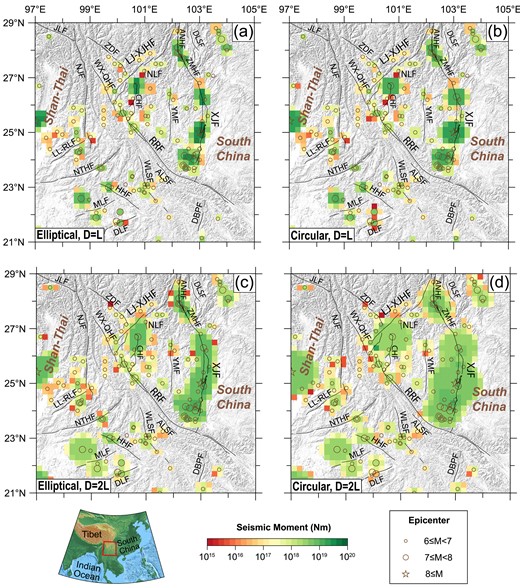
The spatial distribution of epicentres and seismic moments of historical earthquakes in the southeastern Tibetan Plateau after declustering. (a) The seismic moment distribution derived from elliptical area model with major axis equal to fault length (D = L). (b) The seismic moment distribution derived from circular area model with major axis equal to fault length (D = L). (c) The seismic moment distribution derived from elliptical area model with semi-major axis equal to fault length (D = 2 L). (d) The seismic moment distribution derived from circular area model with semi-major axis equal to fault length (D = 2 L). The stars and circles represent the epicentres of M ≥ 6 earthquakes from AD 624 to 2015 after declustering (data are from ISC, the CENC and the Department of Earthquake Disaster Prevention, State Seismological Bureau 1995; Department of Earthquake Disaster Prevention, China Earthquake Administration 1999). The solid lines indicate Quaternary faults. ALSF = Ailaoshan fault; ANHF = Anninghe fault; CHF = Chenghai fault; DBPF = Dien Bien Phu fault; DLF = Daluo fault; DLSF = Daliangshan fault; HHF = Heihe fault; JLF = Jiali fault; LJ-XJHF = Lijiang–Xiaojinhe fault; LL-RLF = Longling–Ruili fault; MLF = Menglian fault; NJF = Nujiang fault; NLF = Ninglang fault; NTHF = Nantinghe fault; RRF = Red River fault; WLSF = Wuliangshan fault; WX-QHF = Weixi–Qiaohou faults; YMF = Yuanmou fault; ZDF = Zhongdian fault and ZMHF = Zemuhe fault.
3.1.2 Spatial distribution of historical seismic moments in the southeastern Tibetan Plateau
First, we calculate the scalar seismic moment Mo (in N·m) for each historical earthquake selected in Section 3.1.1, using the relationship between the scalar seismic moment (Mo) and surface wave magnitude (Ms) in the Tibetan Plateau proposed by Wang et al. (2010), as the following eq. ()
Next, we adopt the elliptical model as described in Section 2.2 as a simplified representation of the seismic area in the southeastern Tibetan Plateau. The geometric centre of the ellipse corresponds to the epicentre, with its (semi-)major axis aligned with the fault strike. The length of the (semi-)major axis is determined by the fault length (L). The fault length (L) is calculated using the relationship between moment magnitude (Mw) and surface wave magnitude (Ms) for the Tibetan Plateau region proposed by Wang et al. (2010), as shown by above eq. (), as well as the relationship between fault length (L) and moment magnitude (Mw) given by Blaser et al. (2010), as shown by above eq. (6). In comparison, we also take a circular area model (Nishimura 2022) into account to identify which seismic area model is more appropriate
After the above processing, we obtain the distribution of seismic areas for M ≥ 6.0 historical earthquakes (AD 624–2015) in the southeastern Tibetan Plateau, as shown in Fig. 3. Finally, we allocate the seismic moment of each earthquake to the grid cells surrounding the epicentre, following that the seismic moment assigned to each cell is proportional to the seismic area within that cell. Finally, the spatial distribution of seismic moments used for retrospective testing in the SASM-test is shown as coloured squares in Fig. 2 and Fig. S1 (Supporting Information).
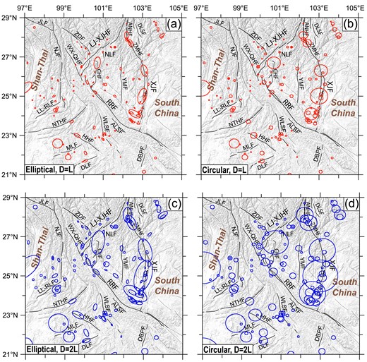
Seismic area distribution of historical earthquakes in the southeastern Tibetan Plateau after declustering. The circles and ellipses represent seismic area. (a) Elliptical area model with major axis equal to fault length (D = L). (b) Circular area model with major axis equal to fault length (D = L). (c) Elliptical area model with semi-major axis equal to fault length (D = 2 L). (d) Circular area model with semi-major axis equal to fault length (D = 2 L).
3.1.3 Earthquake forecasting models evaluation
We test the recently established RELM-TibetSE models (Wei et al. 2023), which are time-independent earthquake forecasting models for M ≥ 6.0 earthquakes in southeastern Tibetan Plateau, developed using Global Navigation Satellite System (GNSS) strain rates and seismicity. The RELM-TibetSE models, which encompasses six probabilistic submodels, that is, UNI 1–3 and VARI 1–3, provide 30-yr probability for M ≥ 6.0 earthquakes. We use the 30-yr probability as the alarm function. The coloured cells in Fig. 4 represent the values of the alarm function.
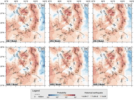
Alarm function values of the RELM-TibetSE models. The alarm function represents the probability of M ≥ 6 earthquakes over future 30 yr. The UNI submodels (a)–(c) are derived from uniform seismogenic layer thickness and rigidity. The VARI submodels (d)–(f) are derived from the seismogenic layer thickness and rigidity with spatial variations. UNI-1 and VARI-1 established using maximum engineering shear strain rate. UNI-2, VARI-2, UNI-3 and VARI-3 established using maximum and minimum principal strain rates in the horizontal plane.
UNI submodels had uniform seismogenic layer thickness and a rigidity, whereas in VARI submodels, the two lithospheric medium parameters were spatially variable. UNI-1 and VARI-1 submodels were established using maximum engineering shear strain rate. UNI-2, VARI-2, UNI-3 and VARI-3 submodels were established using principal strain rates in the horizontal plane. Specifically, the UNI-2 and VARI-2 submodels were established by |$\mathrm{ Max}( {| {\mathop {{{\varepsilon }_1}}\limits^{.} } |,\ | {\mathop {{{\varepsilon }_2}}\limits^{.} } |} )$|, while the UNI-3 and VARI-3 submodels were established by |$\mathrm{ Max}( {| {\mathop {{{\varepsilon }_1}}\limits^{.} } |,\ | {\mathop {{{\varepsilon }_2}}\limits^{.} } |,\ | {\mathop {{{\varepsilon }_1}}\limits^{.} + \mathop {{{\varepsilon }_2}}\limits^{.} } |} )$|. |$\mathop {{{\varepsilon }_1}}\limits^{.} $| and |$\mathop {{{\varepsilon }_2}}\limits^{.} $| denote the maximum and minimum principal strain rates in the horizontal plane. The differences between the six submodels of the RELM-TibetSE are shown in Fig. S2 (Supporting Information).
3.2 Retrospective testing
In addition to the SASM-test, we also employ other classical testing methods from the Collaboratory for the Study of Earthquake Predictability (CSEP), such as the IGPE relative to a reference model with a uniform earthquake distribution (Imoto 2007) and the Molchan-test (Zechar & Jordan 2008), to conduct retrospective statistical testing of the earthquake forecasting models of RELM-TibetSE. The IGPE is the logarithm of the probability gain (G). The probability gain (G) for each earthquake relative to a reference model is calculated using |$G = {\rm{exp}}( {\frac{{L - {{L}_{ref}}}}{N}} )$| (e.g. Helmstetter et al. 2007), where L and |${{L}_{\mathrm{ ref}}}$| represent the log-likelihood of RELM-TibetSE models and the reference model, respectively, and N is the number of earthquakes. The log-likelihood of RELM-TibetSE models is calculated using |$L = \mathop \sum \limits_{i = 1}^K {\rm{log}}[ {{{p}_i}( {l,t} )} ]$|, where |${{p}_i}( {l,t} )$| represents the probability of the ith cell having |$l$| events in period |$t$|, and K is the total number of cells. A higher IGPE value indicates that the forecasted earthquake occurrence probabilities align more closely with actual events, reflecting better model performance. Conversely, a lower IGPE value suggests a poorer forecasting ability of the model.
Fig. 5 illustrates the process of evaluating the submodel UNI-1 of RELM-TibetSE using the SASM-test method. The alarm function values of the UNI-1 submodel are shown in Fig. 5(a). Figs 5(b)–(d) show the alarm regions for three decreased thresholds, and Fig. 5(e) shows the corresponding SASM error diagram. Fig. 6 illustrates the process of evaluating the submodel UNI-1 of RELM-TibetSE using the Molchan-test method. The SASM-test and Molchan-test procedure for other submodels can be found in Figs S3–S12 (Supporting Information).
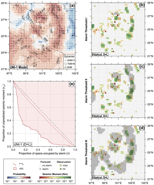
Illustration of retrospective testing using the SASM-test method. (a) Alarm function values of the UNI-1 submodel. (b)–(d) The alarm regions for three decreased thresholds. (e) SASM error diagram of the UNI-1 submodel.
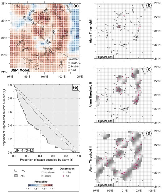
Illustration of retrospective testing using the Molchan-test method. (a) Alarm function values of the UNI-1 submodel. (b)–(d) The alarm regions for three decreased thresholds. (e) Molchan error diagram of the UNI-1 submodel.
The retrospective test results are shown in Fig. 7. In SASM and Molchan error diagrams of the RELM-TibetSE models (Fig. 7), the horizontal axis represents the proportion of space occupied by the alarm. The vertical axis indicates the number of historical earthquakes or the seismic moment in cells without alarms, normalized by the total number of earthquakes and the total seismic moment, respectively. The black solid (τ,|${{\upsilon }_n}$|) curves in Fig. 7 show the results of the original Molchan-test. The red solid (τ,|${{\upsilon }_m}$|) curves in Figs 7(a)–(f) show the miss rates obtained using an elliptical model where the major axis of the ellipse is equal to the fault length (i.e. D = L). The blue solid (τ,|${{\upsilon }_m}$|) curves in Figs 7(a)–(f) show the miss rates obtained using a circular model where the diameter of the circle is equal to the fault length (i.e. D = L). The red solid (τ,|${{\upsilon }_m}$|) curves in Figs 7(g)–(l) show the miss rates obtained using an elliptical model where the semi-major axis of the ellipse is equal to the fault length (i.e. D = 2 L). The blue solid (τ,|${{\upsilon }_m}$|) curves in Figs 7(g)–(l) show the miss rates obtained using an elliptical model where the radius of the circle is equal to the fault length (i.e. D = 2 L).

Molchan error diagrams and SASM error diagrams of the RELM-TibetSE models. The test results using the declustered seismic catalogue. (a)–(f) The test results using the major axis of the ellipse or the diameter of the circle equal to the fault length (D = L). (g)–(l) The test results using the semi-major axis or radius equal to the fault length (D = 2 L). The (τ,|${{\upsilon }_n}$|) curves represented by black (grey) solid curves represent the results of the Molchan-test, with its Y-value normalized by the number of earthquakes. The (τ,|${{\upsilon }_m}$|) curves represented by the red solid step curves indicate the results of the SASM-test, with its Y-value normalized elliptical seismic moment. The (τ,|${{\upsilon }_m}$|) curves represented by the blue solid step curves show the results of the SASM-test, with its Y-value normalized by the circular seismic moment. The dotted step curves indicate 5 per cent confidence level.
In Molchan and SASM error diagrams of the RELM-TibetSE models (Fig. 7), all (τ,|${{\upsilon }_n}$|) and (τ,|${{\upsilon }_m}$|) curves lie below the G = 1 dashed line, indicating that all forecasting models outperform the spatially uniform reference model. For all RELM-TibetSE models, the SASM-test's miss rate (τ,|${{\upsilon }_m}$|) curves (the red lines) are closest to the Y-and X-axes, followed by the circular model's (τ,|${{\upsilon }_m}$|) curves (the blue lines), while the Molchan-test's (τ,|${{\upsilon }_n}$|) curves are farthest away from the Y- and X-axes.
In Figs 7(a)–(f), the red and blue solid (τ,|${{\upsilon }_m}$|) curves are closer to each other, and in Figs 7(g)–(l), the blue solid (τ,|${{\upsilon }_m}$|) curves are closer to the black solid (τ,|${{\upsilon }_n}$|) curves. This indicates that, for any forecasting model, when the seismic area in SASM-test is modelled as an ellipse with its major axis equal to fault length (D = L), the difference between this model and its corresponding circular model is less than that of ellipses modelled with semi-major axis equal to fault length (D = 2 L) and their corresponding circular models.
The statistics of ASS from the SASM-test and Molchan-test (Table 1 and Fig. 8) revealed the performance of five different seismic area parameter applied to six submodels of the RELM-TibetSE. First, the retrospective testing results show that the ASS is highest when modelling the seismic area as an ellipse with the major axis equal to the fault length (D = L), followed by a circle with the diameter equal to the fault length (D = L), then an ellipse with the semi-major axis equal to the fault length (D = 2 L), and lowest when modelled as a circle with the radius equal to the fault length (D = 2 L). Second, the ASS for moment is consistently higher than the ASS for epicentre. Third, as showed in Fig. 8(b), the five miss rate lines exhibit similar shapes without crossing, indicating consistent performance across different parameter settings in these sub-models. The red (τ,|${{\upsilon }_m}$|) curve in Fig. 8(a) fluctuate significantly more than the other miss rate curves, suggesting that the SASM-test method exhibits higher sensitivity when the ellipse's major axis is set equal to the fault length (i.e. D = L). This higher sensitivity may enable better differentiation between similar models. Therefore, we recommend using the parameter where the seismic area is defined as an ellipse with a major axis equal to the fault length (D = L) in SASM-test applications.
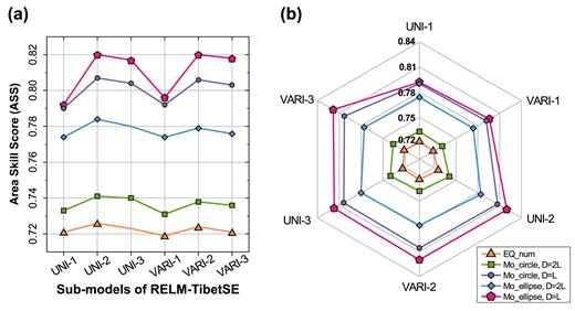
Comparison of ASS for the RELM-TibetSE models. UNI1-3 and VARI1-3 are the submodels of RELM-TibetSE. EQ_num is the ASS for epicentre, Mo_circle is the ASS for moment when the seismic area is modelled as a circle and Mo_ellipse is the ASS for moment when the seismic area is modelled as an ellipse. D = L is the major axis of the ellipse or the diameter of the circle equal to the fault length, and D = 2 L is the semi-major axis of the ellipse or the radius of the circle equal to the fault length.
ASS of the six RELM-Tibet submodels in the retrospective testing
| Test method | Test parameters | UNI-1 | UNI-2 | UNI-3 | VARI-1 | VARI-2 | VARI-3 |
|---|---|---|---|---|---|---|---|
| Molchan-test | EQ_num | 0.721 | 0.726 | 0.723 | 0.719 | 0.724 | 0.721 |
| Mo_circle, D = 2L | 0.733 | 0.741 | 0.740 | 0.731 | 0.738 | 0.736 | |
| Mo_circle, D = L | 0.790 | 0.807 | 0.804 | 0.792 | 0.806 | 0.803 | |
| SASM-test | Mo_ellipse, D = 2L | 0.774 | 0.784 | 0.780 | 0.774 | 0.779 | 0.776 |
| Mo_ellipse, D = L | 0.792 | 0.820 | 0.817 | 0.796 | 0.820 | 0.818 |
Notes. The ASS values range from 0 to 1. EQ_num is the ASS for epicentre, Mo_circle is the ASS for moment when the seismic area is modelled as a circle, Mo_ellipse is the ASS for moment when the seismic area is modelled as an ellipse. D = L is the major axis of the ellipse or the diameter of the circle equal to the fault length and D = 2 L is the semi-major axis of the ellipse or the radius of the circle equal to the fault length.
Finally, the results of the three retrospective statistical tests are presented in Table 2. Comparing these results, we find high consistency between our SASM-test results and those from the widely recognized IGPE and Molchan error diagram. This consistency may suggest a certain degree of reliability and validity in SASM-test method. Additionally, while the IGPE and Molchan-test methods assess, respectively, models from the perspectives of information gain and epicentre alarming ability, the SASM-test provides a new perspective by evaluating alarms for the seismic source area. This comparison results also show that the SASM-test can be consistent with previous methods and can be applied to the evaluation of earthquake forecasting models.
Statistical results of retrospective testing.
| Method | UNI-1 | UNI-2 | UNI-3 | VARI-1 | VARI-2 | VARI-3 |
|---|---|---|---|---|---|---|
| IGPE | 0.829 | 0.976 | 0.98 | 0.743 | 0.893 | 0.914 |
| ASS (Molchan-test) * | 0.721 | 0.726 | 0.723 | 0.719 | 0.724 | 0.721 |
| ASS (SASM-test) * | 0.792 | 0.82 | 0.817 | 0.796 | 0.82 | 0.818 |
| Method | UNI-1 | UNI-2 | UNI-3 | VARI-1 | VARI-2 | VARI-3 |
|---|---|---|---|---|---|---|
| IGPE | 0.829 | 0.976 | 0.98 | 0.743 | 0.893 | 0.914 |
| ASS (Molchan-test) * | 0.721 | 0.726 | 0.723 | 0.719 | 0.724 | 0.721 |
| ASS (SASM-test) * | 0.792 | 0.82 | 0.817 | 0.796 | 0.82 | 0.818 |
The values range from 0 to 1. IGPE is information gain per earthquake of RELM-TibetSE models over a reference model assuming seismic uniform distribution; ASS (Molchan-test) is area skill score for epicentre and ASS (SASM-test) is area skill score for moment when the seismic area is modelled as an ellipse with the major axis equal to the fault length (i.e. D = L).
4 DISCUSSION
4.1 Characteristics of the SASM-test
Using the SASM-test method to evaluate earthquake forecasting models, the evaluation results only indicate forecasting performance of the tested models, but cannot reflect the quality of the testing method itself. For example, the evaluation of the six RELM-TibetSE submodels shown in Fig. 8 indicates that the UNI-2 and VARI-2 submodels have the highest ASS in all five tests, demonstrating the best forecasting performance of the UNI-2 and VARI-2 submodels. However, the red miss rate curves having higher ASS than other miss rate curves do not imply that the SASM-test method is better than Molchan-test method.
To analyse the discriminating ability of various testing methods (or testing parameters) in evaluating earthquake forecasting models, we calculate the variation coefficient of the retrospective testing results of the six similar submodels of RELM-TibetSE in the five testing methods, and we generate the comparative box plots as shown by Fig. 9. Specifically, Fig. 9 indicates that, if the seismic area in the SASM-test method is modelled as an ellipse with the major axis equal to the fault length (D = L), the coefficient of variation was largest. This suggests that model's forecasting sensitivity was largest in this case, resulting in a largest dispersion in the evaluation results of similar models as shown by the pink box. Such high sensitivity could enable better discrimination among similar models. In contrast, the Molchan-test shows the lowest coefficient of variation, as shown by the orange box with shorter box heights and whiskers, indicating that the distribution of the ASS is more concentrated, and the evaluation results of similar models are more consistent. Moreover, if the seismic area is modelled as a circular shape with a radius equal to twice the fault length (D = 2 L) (green box) and as a circular shape with a diameter equal to the fault length (D = L) (blue box), the results show moderate coefficients of variation and box heights, indicating that, in these two cases, SASM-test method provides a balance between discriminating ability and evaluation consistency.
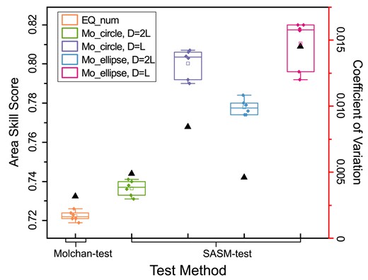
Comparison of ASS box plots and coefficient of variation for evaluating forecasting ability of different testing methods. The diamonds represent the ASS of the six submodels of RELM-TibetSE using the SASM-test or Molchan-test methods. The triangles represent coefficients of variation. Boxes represent the distribution of the ASS obtained by evaluating the six similar forecasting submodels using different testing method or testing parameter.
Overall, the SASM-test method demonstrates higher sensitivity than the Molchan-test method, particularly when the seismic area in the SASM-test is modelled as an elliptical shape with the major axis equal to the fault length (D = L). In this case, the SASM-test method may have an advantage in discriminating the performance subtlety of similar earthquake probabilistic forecasting models.
Additionally, although the proposed SASM-test method exhibits consistency with the classical IGPE and Molchan-test methods in evaluating earthquake forecasting models, the method is characterized by several novelties. This high level of consistency suggests that the SASM-test method can effectively reflects the assessment results of existing approaches and offer deeper insights, thereby adding a new perspective to the evaluation of earthquake forecasting models. Specifically, one key novelty of the SASM-test method lies in its approach to testing the entire seismic source area as the target for evaluation, rather than being limited to the epicentre alone. This is different from the Molchan-test method, which focuses solely on the epicentre. The SASM-test method complements the Molchan-test by capturing the seismic source area and thus can provide additional perspective for evaluating earthquake forecasting models. This approach expands the spatial area of the assessment and may identify details that are difficult to be discerned with Molchan-test method.
4.2 Implications from SASM-test results for refining forecasting models
In this study, we have conducted retrospective testing on the RELM-TibetSE forecasting models using the SASM-test and Molchan-test methods, obtaining two ASS, respectively. The ASS obtained from the SASM-test method, referred to as ‘ASS for moment,’ primarily reflects the model's ability in forecasting the seismic source area. In contrast, the ASS obtained from the Molchan-test method, known as ‘ASS for epicentre,’ reflects the model's ability in forecasting the epicentre location. Comparing the ASS (as shown in Table 1 and Fig. 8) from the six RELM-Tibet submodels in the retrospective testing, we find that the ASS for epicentre is consistently lower than the ASS for moment for all models. This result indicates that earthquake forecasting models based on GNSS strain rates exhibit better performance in forecasting the seismic source area, compared to epicentre location forecasting.
These findings have several implications. First, the spatial distribution of GNSS strain rates more directly reflects the cumulative effects of crustal deformation, making it more suitable for forecasting broader seismic source regions. In contrast, the precise forecasting of epicentre locations may require more complex models or additional information, such as historical earthquake data or local lithospheric structure. Therefore, models based on GNSS data are likely to provide more reliable results in forecasting seismic source regions, while they may be relatively less effective in forecasting specific epicentre locations. These findings further support the effectiveness of GNSS data in earthquake forecasting, particularly in source region forecasting, suggesting that incorporating geodetic data in developing earthquake forecasting models could enhance the accuracy of epicentre location forecasting.
Furthermore, we find that, regardless of whether the Molchan-test or SASM-test method is used to evaluate the six RELM-Tibet forecasting submodels, the ASS for the UNI-2, VARI-2, UNI-3 and VARI-3 submodels are consistently higher than those for the UNI-1 and VARI-1 submodels. This result suggests that the forecasting models based on GNSS principal strain rate may outperform those based on GNSS maximum shear strain rate in both epicentre location forecasting and seismic source area forecasting. The superiority of the former submodels might be attributed to that GNSS principal strain rates can capture large-scale, continuous deformation patterns of the crust, providing more comprehensive characterization of tectonic deformation. In contrast, the maximum shear strain rate is more sensitive to localized stress accumulation along faults or fracture zones, which, while important, may not fully represent the broader tectonic processes driving seismic activity. The former submodels are potentially more suitable for large-scale source region forecasting, thereby being advantageous in earthquake forecasting accuracy and reliability. Additionally, this finding suggests that closer attention should be paid to the selection of strain rate components in the development and evaluation of earthquake forecasting model. For large-area earthquake forecasting, the models based on principal strain rate may result in more accurate forecasts. However, in more localized forecasts that require the capturing intricate fault structures and areas of concentrated stress, the models based on maximum shear strain rate may be more advantageous, as they are more sensitive to small-scale variations and localized stress accumulation that play a key role in seismogenic processes. Overall, this result provides deep insights for optimizing earthquake forecasting models based on GNSS data, suggesting that it is justified to further explore the impact of different strain rate components on model performance in future studies.
Table 2 presents the statistical results of the retrospective testing of the six RELM-Tibet submodels using various testing methods. The results indicate that the IGPE and Molchan-test methods, which primarily assess epicentre forecasting ability, yielded slightly higher statistical results for the UNI submodels which were developed with uniformly distributed seismogenic layer thickness and rigidity, compared to the VARI submodels based on spatial variations in seismogenic layer thickness and rigidity. In contrast, in the SASM-test method, which is characterized by evaluating seismic source area forecasting ability, the statistical results for the UNI submodels were lower than or equal to those for the VARI submodels. In addition to comparing the ASS results evaluated by the SASM-test and Molchan-test methods, we also calculate the percentage of earthquakes forecasted in the top 30 per cent highest probability cells of the forecasting models, indicated by the proportion of unforecasted seismic number or seismic moment at x = 0.3 in the SASM or Molchan error plots (Fig. 10), to compare the models' forecasting performance. According to the intersection of the grey dashed line with the light blue and orange miss rate curves in Fig. 10, the Molchan-test results show that 65.9 per cent of historical earthquake epicentres are located within the top 30 per cent highest probability grids of the UNI-2 submodel, while this proportion was 66.7 per cent for the VARI-2 submodel. On the other hand, the SASM-test results show that 77.9 per cent of historical seismic moments are located within the top 30 per cent highest probability grids of the UNI-2 submodel, while this proportion is 81.6 per cent for the VARI-2 submodel (see Table 3) as indicated by the intersection of the grey dashed line with the red and dark blue miss rate curves in Fig. 10. These findings suggest that incorporating spatial variations in seismogenic layer thickness and rigidity into the forecasting models, as opposed to using uniform seismogenic layer thickness and rigidity, may significantly enhance the model's ability in forecasting the ‘seismic source area.’ This further supports the necessity of introducing spatial heterogeneity lithospheric properties into earthquake forecasting models to improve their forecasting accuracy.
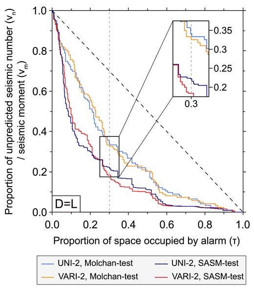
SASM and Molchan error diagrams of UNI-2 submodel compared with VARI-2 submodel.
Statistical results of retrospective testing for UNI-2 and VARI -2 submodels.
| Submodel | Molchan-test | SASM-test | ||
|---|---|---|---|---|
| ASS for epicentre* | Proportion of epicentre concentration* | ASS for moments* | Proportion of moment concentration* | |
| UNI-2 | 0.726 | 0.659 | 0.820 | 0.779 |
| VARI-2 | 0.724 | 0.667 | 0.820 | 0.816 |
| Submodel | Molchan-test | SASM-test | ||
|---|---|---|---|---|
| ASS for epicentre* | Proportion of epicentre concentration* | ASS for moments* | Proportion of moment concentration* | |
| UNI-2 | 0.726 | 0.659 | 0.820 | 0.779 |
| VARI-2 | 0.724 | 0.667 | 0.820 | 0.816 |
*The parameter values range from 0 to 1. ASS is area skill score; proportion of epicentre or moment concentration is the proportion of forecasted earthquakes in cells of the upper 30 per cent of high alarms.
It should be mentioned that the seismogenic layer model used by Wei et al. (2023) does not have a high spatial resolution, far from matching the spatial resolution of 0.2° × 0.2° of the forecasting models (i.e. RELM-TibetSE). If a higher resolution seismogenic layer model for the southeastern Tibetan Plateau is available in the future, the RELM-TibetSE established using spatially variable seismogenic layer data might have higher forecasting performance.
5 CONCLUSIONS
In this study, we propose a novel statistical method, the SASM-test, for evaluating earthquake forecasting models. This method addresses the limitations of conventional approaches, such as the Molchan-test, which focus solely on the epicentre location, by introducing the seismic source area. We apply this method to the recently developed earthquake forecasting models of RELM-TibetSE for south-eastern Tibet. The evaluation results demonstrates that the SASM-test exhibits higher sensitivity in the retrospective testing of the seismic forecasting models, particularly when the seismic area is modelled as an ellipse with the major axis equal to the fault length (D = L). The SASM-test proves to be more effective in discriminating the performance subtlety of similar earthquake forecasting models.
Comparing the statistical results obtained from retrospective testing using the SASM-test method, we obtain the following findings: (i) RELM-TibetSE based on GNSS strain rates exhibits higher accuracy in forecasting the source region compared to forecasting the epicentre location; (ii) seismic forecasting models developed with GNSS principal strain rates involved outperform those based on GNSS maximum shear strain rate in both epicentre location forecasting and source area forecasting, possibly due to that principal strain rates better capture large-scale, continuous crust deformation patterns, whereas the maximum shear strain rates, though more sensitive to localized stress accumulation along faults, may not fully represent the tectonic processes driving seismic activity and (iii) If taking spatial heterogeneity lithospheric properties into account, such as spatially varying seismogenic layer thickness and rigidity, we can enhance the performance of seismic forecasting models in source region forecasting.
In conclusion, the proposed SASM-test method can supplement the evaluation techniques for earthquake forecasting models, highlighting the advantages of forecasting models developed based on GNSS data and the spatial heterogeneity of lithospheric properties. These findings may further advance the development of more accurate and effective earthquake forecasting models, and contribute to improve seismic hazard assessments and risk management.
ACKNOWLEDGMENTS
This study is financially supported by National Key R&D Program of China (2019YFE0108900), National Natural Science Foundation of China (42374009, 42304008 and 41874024) and Special Fund of Institute of Earthquake Forecasting, China Earthquake Administration (CEAIEF20240404). We thank editor Margarita Segou, reviewer Matteo Taroni, and an anonymous reviewer for their insightful comments, which have significantly improved our manuscript. We sincerely thank Professor Mengtan Gao for the valuable insights gained through prior discussions, which inspired the development of the methodology in this study. We acknowledge earthquake catalogues provided by the China Earthquake Networks Center (CENC), the International Seismological Centre (ISC) and the Global Centroid Moment Tensor (GCMT) Project.
DATA AVAILABILITY
The earthquake catalogues are collected from CENC available at http://data.earthquake.cn/, the Department of Earthquake Disaster Prevention, State Seismological Bureau (1995), the Department of Earthquake Disaster Prevention, China Earthquake Administration (1999) and the reference of Xu & Gao (2014). The Earthquake catalogue of Myanmar and Laos are extracted from the ISC, Online Bulletin at 30: 10.31905/D808B830, GCMT Project available at https://www.globalcmt.org/, and the publication of Wang et al. (2014). The alarm function of RELM-TibetSE model is obtained from Wei et al. (2023). The fault data are downloaded from the SAFSDC (https://www.activefault-datacenter.cn/). Partial plots were generated using the Generic Mapping Tools (GMT) version 5.3.3 (Wessel et al. 2013).
