


SUMMARY
Within the Western Branch of the East African Rift (EAR), volcanism is highly localized, which is distinct from the voluminous magmatism seen throughout the Eastern Branch of the EAR. A possible mechanism for the source of melt beneath the EAR is decompression melting in response to lithospheric stretching. However, the presence of pre-rift magmatism in both branches of the EAR suggest an important role of plume-lithosphere interactions, which validates the presence of voluminous magmatism in the Eastern Branch, but not the localized magmatism in the Western Branch. We hypothesize that the interaction of a thermally heterogeneous asthenosphere (plume material) with the base of the lithosphere enables localization of deep melt sources beneath the Western Branch where there are sharp variations in lithospheric thickness. To test our hypothesis, we investigate sublithospheric mantle flow beneath the Rungwe Volcanic Province (RVP), which is the southernmost volcanic center in the Western Branch. We use seismically constrained lithospheric thickness and sublithospheric mantle structure to develop an instantaneous 3D thermomechanical model of tomography-based convection (TBC) with melt generation beneath the RVP using ASPECT. Shear wave velocity anomalies suggest excess temperatures reach ∼250 K beneath the RVP. We use the excess temperatures to constrain parameters for melt generation beneath the RVP and find that melt generation occurs at a maximum depth of ∼140 km. The TBC models reveal mantle flow patterns not evident in lithospheric modulated convection (LMC) that do not incorporate upper mantle constraints. The LMC model indicates lateral mantle flow at the base of the lithosphere over a longer interval than the TBC model, which suggests that mantle tractions from LMC might be overestimated. The TBC model provides higher melt fractions with a slightly displaced melting region when compared to LMC models. Our results suggest that upwellings from a thermally heterogeneous asthenosphere distribute and localize deep melt sources beneath the Western Branch in locations where there are sharp variations in lithospheric thickness. Even in the presence of a uniform lithospheric thickness in our TBC models, we still find a characteristic upwelling and melt localization beneath the RVP, which suggest that sublithospheric heterogeneities exert a dominant control on upper mantle flow and melt localization than lithospheric thickness variations. Our TBC models demonstrate the need to incorporate upper mantle constraints in mantle convection models and have global implications in that small-scale convection models without upper mantle constraints should be interpreted with caution.
1 INTRODUCTION
The Eastern Branch of the East African Rift (EAR; Fig. 1a) includes widespread magmatism with flood basalts extending hundreds of kilometers. For example, the Kenyan Rift alone in the Eastern Branch has an estimated 924 000 km3 of mafic magma and underplated material generated in the past 30 Ma (Latin et al. 1993). However, the Western Branch (Fig. 1a) is characterized by limited and sparse magmatism and the reason for this dichotomy in melt volume between the Eastern Branch and Western Branch is not well understood (e.g. Rosenthal et al. 2009; Hudgins et al. 2015; O'Donnell et al. 2016; Njinju et al. 2021), partly because existing geodynamic models do not incorporate upper mantle heterogeneities constraints from observations (Njinju et al. 2021). Previous studies suggest that the localized magmatism in the Western Branch results from decompression melting in response to lithospheric stretching (e.g. Yu et al. 2020). However, there is geochemical evidence of pre-rift magmatism in the Eastern Branch and Western Branch of the EAR (Roberts et al. 2012; Mesko et al. 2014; Mesko 2020; Rooney 2020), which suggest that sublithospheric melt generation beneath the entire EAR is more importantly generated from thermal perturbations in the asthenosphere rather than decompression melting in response to lithospheric stretching. Koptev et al. (2016, 2018) developed fully coupled thermomechanical models which suggest that the position of the Eastern Branch, the Western Branch and the Malawi Rift with respect to the Tanzanian and Bangweulu Cratons can be explained by a non-uniform splitting of the Kenyan plume, which has been rising underneath the southern part of the Tanzanian Craton. Thus, asthenospheric processes play an important role in the generation and localization of sublithospheric melt beneath the Western Branch. The development of a geodynamic model that incorporates asthenospheric heterogeneities (complex plume geometry) constraints from observations is therefore necessary in order to understand the origin of the localization of magmatism in the Western Branch of the EAR. Such geodynamic models with a complex plume geometry will complement the Koptev et al. (2016, 2018) studies, which implement a rather simple plume geometry. We therefore hypothesize that the interaction of a thermally heterogeneous asthenosphere (plume material) with the base of the lithosphere enables localization of deep melt sources beneath the Western Branch where there are sharp variations in lithospheric thickness.
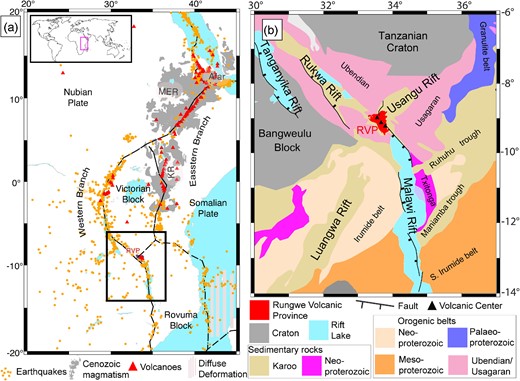
(a) Map of the EAR showing the Eastern and Western Branches. The Western Branch of the EAR has fewer volcanic centers (red triangles are Holocene volcanoes) and more earthquakes (orange dots are earthquakes with >M2) than the Eastern Branch. The Holocene volcanoes are from the Smithsonian Global Volcanism Project and the earthquakes are from the NEIC catalog (Beauval et al. 2013). The Cenozoic volcanic rocks (gray) are outlined after Thiéblemont et al. (2016) and indicate the large igneous province in East Africa. RVP = Rungwe Volcanic Province. KR = Kenyan Rift. MER = Main Ethiopian Rift. The black rectangle shows the location of Fig. 1(b). Dashed lines represent plate boundaries from Stamps et al. (2008). RVP lies at the Mbeya triple junction. The inset map shows the relative location of part of the EAR (pink rectangle) on Earth. The diffuse deformation offshore of the Eastern Branch is based on a geodetic study by Stamps et al. (2021). (b) Map of major terranes and geological features in the southern part of the Western Branch of the EAR that are based on Fritz et al. (2013). The major rift faults are extracted from Muirhead et al. (2019). Black triangles from north to south represent the three large active volcanoes (Ngozi, Rungwe and Kyejo; Fontijn et al. 2010; Harkin 1960) of the RVP.
To test our hypothesis, we investigate sublithospheric mantle flow beneath the Rungwe Volcanic Province (RVP; Fig. 1b), which is the southernmost volcanic center in the Western Branch of the EAR. The RVP provides a natural laboratory to investigate the role of asthenospheric processes in the generation and localization of melt in the magma-poor Western Branch. The RVP lies at the triple junction formed by the Rukwa Rift, Malawi Rift and the Usangu Rift (Fig. 1a and b), which may link the magma-rich Eastern Branch to the Western Branch of the EAR (Purcell 2018). The RVP lies within the 1.8 Ga Ubendian-Usagaran mobile belts that circumvent the thick lithosphere of the Tanzanian and Bangweulu cratons (Fig. 1b; e.g. Corti et al. 2007; Fritz et al. 2013; Bahame et al. 2016; Ganbat et al. 2021) and consists of three large volcanoes, Ngozi, Rungwe and Kyejo that were, respectively, last active about 1 ka (erupted trachytic tuff), 1.2 ka (erupted trachytic tephra) and 0.2 ka (erupted tephrite lava flow; Harkin 1955; Ebinger et al. 1989; Fontijn et al. 2010, 2012; black triangles, Fig. 1b). Magmatism in the RVP is highly localized with past eruptions covering ∼1500 km2 (Fig. 1b; Ebinger et al. 1989, 1997; Fontijn et al. 2012). 40Ar/39Ar radiometric dating of samples from the RVP suggest that magmatism in the RVP started at least by 19 Ma (Mesko et al. 2014; Mesko 2020) and possibly as early as ∼25 Ma (Roberts et al. 2012), which predates rifting in the northern Malawi Rift that started at ∼8.6 Ma (Ebinger et al. 1993) and the reactivation of the Rukwa Rift at ∼8.7 Ma (Hilbert-Wolf et al. 2017). These ages suggest that magmatism in the RVP might have played an important role in thermally weakening the lithosphere, thereby facilitating rifting, yet the sublithospheric mantle flow fields and deep melt source beneath the RVP have not been well constrained (i.e. Furman 1995; Fontjin et al. 2012; Kimani et al. 2021; Njinju et al. 2021). A previous investigation of lithospheric modulated convection (LMC) and deep melt generation beneath the RVP by Njinju et al. (2021), just like with most small-scale convection models, did not include constraints of the upper mantle structure and is thus suffering from an information gap.
Here, we develop an instantaneous 3D thermomechanical model of tomography-based convection (TBC) and melt generation beneath the RVP using the finite element code ASPECT (Advanced Solver for Problems in Earth's ConvecTion; Dannberg & Heister 2016; Heister et al. 2017; Bangerth et al. 2018a, b). TBC is defined as a model of mantle convection that is generated from temperature variations derived from seismic velocity perturbations. We impose a laterally varying rigid lithosphere (Fishwick 2010) with an approximately conductive geotherm that is modeled as a linear gradient from the surface (293 K) to the base of the lithosphere [TLAB; temperature at lithosphere-asthenosphere boundary (LAB)], which is an adiabatic boundary defined by the mantle potential temperature (Tp; McKenzie & Bickle 1988). For the sublithospheric mantle, we implement an adiabatic background temperature with additional temperature perturbations derived from shear wave seismic velocity constraints from Emry et al. (2019). We also use rheological flow laws that account for melt generation in a continental setting following Njinju et al. (2021).
We find upwelling asthenosphere from TBC beneath the RVP where the lithosphere is relatively thin and slow seismic velocity anomalies are present. We test the competing role of sublithospheric heterogeneities and the effect of lithospheric thickness variations on upper mantle flow by replacing the lithospheric thickness model with a uniform 100-km thick lithosphere and compare the resultant flow fields with those from the TBC model and find similar flow patterns. The TBC models reveal mantle flow patterns not evident in LMC models such as upwelling beneath the Tanzanian Craton and corner flow adjacent to the Bangweulu Craton. Our results show that with a seismically derived excess temperature of ∼250 K beneath the RVP, upwelling from TBC generates melt at a maximum depth of ∼140 km beneath the RVP. Our results suggest that upwelling from a thermally heterogeneous asthenosphere distributes and localizes deep melt sources beneath the Western Branch where the lithosphere is thin. Our TBC models suggest a dominant control of sublithospheric heterogeneities on upper mantle flow and melt localization than lithospheric thickness variations, which demonstrates the need to incorporate upper mantle constraints in mantle convection models. Thus, there should be caution in the interpretation of small-scale convection models that do not incorporate upper mantle constraints.
2 METHODS
We model instantaneous TBC in a 3D regional domain that incorporates melt generation in the sublithospheric mantle beneath the RVP using the finite element code ASPECT (Dannberg & Heister 2016; Heister et al. 2017; Bangerth et al. 2018a, b); to test the hypothesis that the interaction of a thermally heterogeneous asthenosphere with the base of the lithosphere enables localization of deep melt sources beneath the Western Branch where there are sharp variations in lithospheric thickness.
2.1 3D TBC modeling
2.1.1 Governing equations
We simulate an instantaneous TBC model for an incompressible Newtonian viscous fluid by solving for the mantle flow fields, u and pressure, p, in the conservation of momentum (eq. 1) and conversation of mass (eq. 2) equations.
where ε(u), η, g and |$\rho $| are, respectively, the strain rate, viscosity, gravitational acceleration and density. We assume a uniform crustal density of 2700 kg m−3 in the model with a uniform thickness of 30 km (after Rajaonarison et al. 2020). For the lithospheric mantle, we assume a uniform density of 3400 kg m−3. We apply the Boussinesq approximation, which neglects small density variations in the model except for the buoyancy term (right-hand side of the momentum equation, eq. 1) in the sublithospheric mantle where the density varies with both temperature and pressure (T and p; eq. 3).
where |${\rho }_{solid}$| is the density of solid rocks, |${\rho }_{melt}$| is the density of melt, α is the thermal expansivity and |${\rho }_{0}$| is the reference density at reference temperature, |${T}_0$| and reference pressure, |${p}_{0}$|. |${\rho }_{0}$| = 3300 kg m−3 for solid rocks and |${\rho }_{0}$| = 3000 kg m−3 for melts. We normalize the pressure to a surface pressure of |${p}_{0}$| = 105 Pa where |${T}_{0}$| = 293 K (Yang et al. 2018; Njinju et al. 2021). For the Earth's mantle, α = 3.0 × 10⁻⁵ K−1 and β = 4.2 × 10⁻¹² Pa−1. We however, test the effect of mantle compressibility in the density model by comparing the density structure with a density model without mantle compressibility (i.e. β = 0 Pa−1) and find that there is significant increase in density when we include mantle compressibility with density residuals reaching ∼75 kg m−3 at 150 km depth and reaching >120 kg m−3 at deeper depths (>250 km) in the sublithospheric mantle (see Fig. S1).
We consider melt buoyancy in the sublithospheric mantle by assuming a reference density defined by the effective density of partially molten rocks (|${\rho }_{eff}$|), i.e.:
where F is the melt fraction (see Section 2.2 below).
2.1.2 Model setup
We use seismically constrained lithospheric structure (Fig. 2a; Fishwick 2010) and shear wave velocity perturbations in the sublithospheric mantle (Fig. 2b; Emry et al. 2019) to define the temperature fields of the model. The lithosphere is thinnest beneath the RVP (∼100–120 km) and thickest beneath the central to southern segment of the Malawi Rift (∼175–200 km). These thicknesses are consistent with gravity-derived lithospheric depth estimates in Njinju et al. (2019a).
We assume an approximately conductive geothermal temperature distribution for the lithosphere by implementing a linear temperature gradient from the surface (T0 = 293 K) to the base of the lithosphere (TLAB), which is an adiabatic boundary defined by the Tp (eq. 5 derived from the adiabatic temperature gradient |${( {\frac{{\partial T}}{{\partial z}}} )}_s = \frac{{\alpha Tg}}{{{C}_p}}\ $|; McKenzie & Bickle 1988).
where g,|$\ \alpha $|, |${z}_{LAB}$| and |${C}_p$| is, respectively, the gravitational acceleration, thermal expansivity, depth to the LAB and specific heat. For the Earth's sublithospheric mantle we define Cp = 1250 J.kg−1. K−1 following Dannberg & Heister (2016). The variable lithospheric thickness (Fig. 2a; Fishwick 2010) produces lateral variations in temperature and pressure, which leads to lateral density perturbations in the sublithospheric mantle. Fig. 2(c) shows lateral variations of the LAB temperatures beneath the RVP and surroundings derived from eq. (5) for ambient mantle potential temperature of 1200° C (1473 K). Unlike studies that suggest the LAB to be a 1300° C isotherm (e.g. Artemieva 2006; Koptev & Ershov 2011), we consider the LAB to be an adiabatic boundary with lateral variations in temperatures (∼1510–1545 K; Fig. 2c). The insulating effect of the LAB following the adiabatic boundary assumption is such that the thin lithosphere beneath the RVP (Fig. 2a) is characterized with low LAB temperatures (<1515 K; Fig. 2c) and regions with thick lithosphere (Fig. 2a) are characterized with elevated LAB temperatures (>1535 K; Fig. 2c).
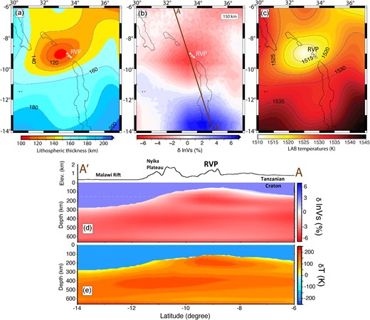
(a) Lithospheric thickness map of the RVP (white triangles) and surroundings, updated from Fishwick (2010), which we use as input in this study. Contours show lines of equal lithospheric thickness at 20 km intervals. The thinnest lithosphere (∼100 km) adjacent to RVP occurs beneath the Mbeya triple junction. Black lines indicate the outline of rift lakes. (b) 150 km depth slice of seismic velocity perturbation derived from Emry et al. (2019). The velocities are relative to the AK135 global average Earth Model (Kennett et al. 1995). Brown line AA′ is the profile location for Fig. 2(c) and (d). (c) LAB temperatures beneath the RVP and surroundings for ambient mantle potential temperature of 1200° C (1473 K). (d) Cross-section of seismic velocity perturbation after Emry et al. (2019) along profile AA′. The velocities are relative to the AK135 global average Earth Model (Kennett et al. 1995). (e) Temperature anomalies derived from the velocity perturbations are in Fig. 2(c).
We derive excess temperatures in the sublithospheric mantle from shear wave velocity anomalies. We first convert the shear wave velocity anomalies |$\delta $|vs/vs from Emry et al. (2019) to the equivalent density perturbations |$\delta $|ρ/ρ using a velocity-density conversion factor of 0.20 using eq. (6a). The conversion of shear wave velocity anomalies to density perturbations is based on the assumption that the shear wave velocity anomalies are due to temperature variations only (e.g. Hager & Richards 1989; Lithgow-Bertelloni & Silver 1998). For example, Becker (2006), Conrad & Lithgow-Bertelloni (2006) and Conrad & Behn (2010) use a conversion factor between shear wave velocity anomalies and density anomalies of 0.15, while Ghosh et al. (2010, 2017) and Wang et al. (2015) assume a conversion factor of 0.25. The limitations of the conversion of shear wave velocity perturbations to density perturbations through the design of a simple velocity-density conversion factor have been examined by Adam et al. (2021) and Njinju et al. (2023). In order to limit the complexity of our model setup, we however, adopt a simple approach and test a range of velocity-density conversion factors (0.15–0.25). We choose 0.20, which generates realistic melt fractions for the sublithospheric mantle (see Section 3.1.1 and Table 2). We follow the approach of Austermann et al. (2017) and multiply the derived density perturbations by the negative inverse of thermal expansivity α to obtain the temperature anomaly |$\delta $|T (eq. 6b; Fig. 2d). The temperature of the sublithospheric mantle (TSLM; eq. 7a) thus consists of a sublithospheric background temperature (TSLB; eq. 7b) with an additional temperature perturbation (|$\delta $|T) derived from shear wave velocity anomalies (Fig. 2b and d; Emry et al. 2019). We note that the shear wave velocity perturbations from Emry et al. (2019) are relative to the AK135 global average Earth Model (Kennett et al. 1995) so ideally, the sublithospheric background temperature (TSLB) should be consistent with the AK135 global average Earth Model (Kennett et al. 1995). However, we make our model simple by allowing TSLB to increase adiabatically to the base of the model (McKenzie & Bickle 1988).
The temperature anomaly (Fig. 2e) suggests excess temperatures reach ∼250 K in the sublithospheric mantle beneath the RVP where shear wave velocities decrease by 6 per cent.
where the sublithospheric depth, z > zLAB (depth to LAB). TSLB, Tp, TSLM, g, |$\alpha $| and |${C}_p$| is, respectively, the background temperature in the sublithospheric mantle, the mantle potential temperature, the temperature in the sublithospheric mantle, the gravitational acceleration, thermal expansivity and specific heat. The Tp in the RVP ranges from ∼1693 to 1723 K based on geochemical observations (Rooney et al. 2012). We test a range of Tp values in melt generation (see Section 3.1.1). The resultant temperature structure for the TBC model is shown in Fig. 3(a) and (b).
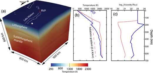
(a) Numerical model setup showing the model dimensions and the temperature structure as the background in 3D for the TBC model with lateral variations in lithospheric thickness. Red triangles represent the RVP. White lines show the outline of rift lakes. (b) Temperature-depth profile beneath the RVP (red line) and beneath the 180 km thick lithosphere in the southern part of the Malawi Rift indicated with a white star in Fig. 3(a) (blue line). Red line represents the 0.4 K km−1 adiabat with mantle potential temperature, Tp. (c) Viscosity-depth profile beneath the RVP (red line) and beneath the white star in Fig. 3(a) (blue line).
Our model domain has dimensions of 800 × 900 × 660 km along latitude, longitude and depth, respectively, for a spherical chunk geometry (Fig. 3a). We refine the entire model domain to a global mesh refinement of 6 such that each element is ∼12 × 14 × 10 km with 17.5 million unknowns computed on 640 cores from Virginia Tech's High-Performance Cluster called Tinkercliffs. We set the velocities at all sides of the model to zero, which exerts minimal edge-effects on the model interior from the boundaries of the model as shown in Njinju et al. (2019a, 2021). The temperature boundary conditions are given by fixed temperatures at the surface and bottom of the model with zero heat flux at the sides of the model (e.g. Rajaonarison et al. 2020). The surface temperature is fixed at 293 K while the temperature at the base of the model is defined by the temperature in eq. 7(a) for z = 660 km.
2.1.3 Rheology
We impose a strong, uniform viscosity of 1023 Pa.s for the lithosphere (Fig. 3c), while for the sublithospheric mantle, we use non-Newtonian, temperature-, pressure- and porosity-dependent creep laws of anhydrous peridotite. The viscosity of the sublithospheric mantle (ηSLM) is given by the multiplication of a porosity dependence factor to a background viscosity governed by the composite rheology of dry olivine material parameters following Rajaonarison et al. (2020). The composite rheology (ηcomp) is the harmonic average of the viscosity from dislocation-creep (ηdisl) and diffusion-creep (ηdiff) flow laws of dry olivine (Jadamec & Billen 2010),
where A is the prefactor, n is the stress exponent, |$\dot{\epsilon }\ $|is the square root of the second invariant of the deviatoric strain rate tensor, d is the grain size, m is the grain size exponent, Ea is the activation energy, Va is the activation volume, p is pressure, R is the gas constant and T is the temperature. The values for the parameters A, n, m, Ea and Va are obtained from experimental studies of dry olivine (Hirth & Kohlstedt 2003; Table 1). The exponential melt-weakening factor is experimentally constrained to 25 ≤αΦ ≤30 (Mei et al. 2002). We use αΦ= 27 following Dannberg & Heister (2016). The porosity Φ is the ratio of the volume of pore spaces between the olivine grains of peridotite to the bulk volume of the peridotite constituent of the asthenosphere. We assume the pore spaces are 100 per cent saturated with melt. The material properties for each layer (lithosphere and sublithospheric mantle) are tracked through compositional fields with the asthenosphere and transition zone further divided into two compositional fields called ‘porosity’ and ‘peridotite’, respectively. Partial melt in the model is tracked through the compositional field ‘porosity’. The viscosity at each quadrature point is calculated from the harmonic average of the compositional fields weighted by the volume fraction of each composition at the same location.
Rheological parameters for dry olivine used in the viscosity flow law of the sublithospheric mantle.
| Parameter | Symbol | Dislocation creep | Diffusion creep | Unit |
|---|---|---|---|---|
| Activation energy | Ea | 530 × 103 | 375 × 103 | J mol−1 |
| Activation volume | Va | 25 × 10−6 | 6 × 10⁻⁶ | m3 mol−1 |
| Grain size | d | – | 10 × 10−3 | m |
| Grain size exponent | m | – | 3 | – |
| Stress exponent | n | 3.5 | 1.0 | – |
| Prefactor | A | 7.4 × 10⁻¹⁵ | 4.5 × 10⁻¹⁵ | Pa−nmms−1 |
The rheological parameters for the sublithospheric mantle are from Hirth & Kohlstedt (2004). The prefactor in Hirth & Kohlstedt (2004) (i.e. A′) is derived from uniaxial strain experiments and is converted to the plane strain equivalent (i.e. A) using the following relationship: |$A\ = \frac{{{3}^{\frac{{n + 1}}{2}}}}{{{2}^{1 - n}}}\ \times {10}^{ - 6( {m + n} )}A^{\prime}$| for dry olivine (Becker 2006).
2.2 Partial melting
We model low extent batch melting of anhydrous lherzolite, which occurs prior to the exhaustion of clinopyroxene. Batch melting is considered melting of an upwelling parcel of mantle rock without instantaneous melt extraction and assumes that the melt fraction only depends on temperature, pressure and how much melt has already been generated at a given point (Ribe 1985; Asimow & Stolper 1999).
We use the melting parameterization by Katz et al. (2003), which is valid for shallow upper mantle melting beneath continental lithosphere at pressures generally less than 13 GPa. Partial melting in the sublithospheric mantle occurs if the Tp is such that an adiabatically ascending mantle intersects the solidus (Fig. 4; McKenzie & Bickle 1988). The derived melt fraction F (p, T) depends on the pressure p (Pa) and temperature T (K) and is given by
where the mantle solidus temperature Tsolidus and liquidus temperature Tliquidus are respectively given by
3 RESULTS
3.1 Tests of mantle potential temperatures, velocity-density conversion factors and the competing roles of lithospoheric thickness variations and sublithospheric heterogeneities in melt generation
3.1.1 Sensitivity tests of mantle potential temperature and velocity-density conversion factor in melt generation
Partial melting in the sublithospheric mantle occurs if the mantle potential temperature Tp and the velocity-density conversion factor are such that the resultant geotherm intersects the solidus (Fig. 4). The derived melt fraction is proportional to the temperature in excess of the solidus. Geochemical observations from the RVP suggest that the Tp in the RVP is elevated and ranges from ∼1420 to 1450° C (∼1693–1723 K; Rooney et al. 2012). However, more recent temperature estimates of olivine thermobarometry from volcanic samples from the RVP range from 1199–1375° C (1472–1648 K; Class et al. 2018; Mesko 2020). These may not represent Tp in the sublithospheric mantle if they are from samples of solidified magma. However, according to Faul & Jackson (2005) and Goes et al. (2012), who applied empirical relationships to model mantle material properties, the temperature range of 1199–1375° C is a reasonable range for normal ambient asthenosphere. We therefore test a wide range of mantle potential temperatures beneath the RVP (Tp = ∼1200–1470° C; 1473–1743 K). The geotherm for Tp = 1473 K is not hot enough to generate melt even after including excess sublithospheric mantle temperatures that we constrain with a shear wave velocity-density conversion factor of 0.15 (Table 2). We further test conversion factors of 0.20 and 0.25 and find that for a conversion factor of 0.20, melt is generated with maximum melt fraction reaching 0.8 per cent and for a conversion factor of 0.25, the maximum melt fraction is 21.1 per cent (Table 2). We also test a geotherm for Tp = 1483 K and conversion factor of 0.20 and generate decompression melts with maximum melt fractions reaching 10.5 per cent (Table 2). Experimental studies by Chantel et al. (2016) on asthenospheric rock samples provide evidence of partial melting in the asthenosphere with melt fractions generally between 0 and 0.5 per cent, which they suggest to be a viable origin for the low velocity zones at the base of the lithosphere. We therefore chose the TBC model with Tp = 1473 K and conversion factor of 0.20 as our preferred model because the maximum melt fraction of 0.8 per cent is more representative of asthenospheric conditions.
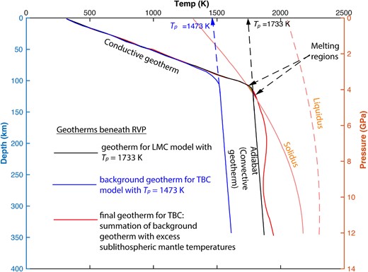
A combined plot of temperature-depth profiles and a pressure-temperature phase diagram depicting shallow melting of anhydrous peridotite parameterized from Katz et al. (2003). Blue-dashed lines represent the geotherm for an ambient mantle (constrained with Tp = 1473 K) beneath the RVP. Red solid line is the geotherm when a tomography-based (Emry et al. 2019) excess temperature is added to the ambient mantle potential temperature (same as temperature structure in Fig. 3b). Black solid line represents the geotherm beneath the RVP constrained with Tp = 1733 K. The orange solid line represents the solidus (0 per cent melt) and the orange-dashed line represents the liquidus (100 per cent melt). The solidus and liquidus are plotted from eqs (9b) and (9c), respectively. Tp represent the mantle potential temperature.
Model tests for different mantle potential temperatures and conversion factors, including the maximum melt fractions generated.
| Model groups | Mantle potential temperatures (K) | Velocity-density conversion factor | Maximum melt fraction (per cent) |
|---|---|---|---|
| TBC | 1473 | 0.15 | 0 |
| – | – | 0.20 | 0.8 |
| – | – | 0.25 | 21.1 |
| – | 1483 | 0.20 | 10.5 |
| LMC | 1723 | – | 0 |
| – | 1733 | – | 0.4 |
| – | 1743 | – | 1.8 |
| TBC-litho100km | 1473 | 0.20 | 0.8 |
The preferred models with their corresponding conversion factors and maximum melt fractions are highlighted in bold. TBC = Tomography-based convection constrained with lithospheric thickness from Fishwick (2010) and shear-wave velocity perturbation from Emry et al. (2019). TBC-litho100km = Tomography-based convection with a uniform 100-km thick lithosphere. LMC = Lithospheric modulated convection constrained with lithospheric thickness from Fishwick (2010).
We test elevated Tp values for models driven by lithospheric thickness variations alone (LMC models) and find that the geotherm for Tp = 1723 K does not generate decompression melt (Table 2). We further test a higher Tp value, that is, Tp = 1733 K and observe that the geotherm crosses the solidus (Fig. 4) producing decompression melt with maximum melt fraction reaching 0.4 per cent (Table 2). For Tp = 1743 K, the maximum melt fraction is 1.8 per cent (Table 2). This test demonstrates that in order to generate decompression melt beneath the RVP, the mantle potential temperature must be elevated (Tp > 1723 K) suggesting a heat source at depth. Shear-wave velocity perturbations from Emry et al. (2019) provides a first order estimate of the excess temperature from this heat source to be up to 250 K.
3.1.2 Test of the competing effects of lithospheric thickness variations and sublithospheric heterogeneities in melt generation
In order to examine the competing effects of lithospheric thickness variations and sublithospheric heterogeneity in melt generation, in addition to the TBC models and the LMC models, we develop a third model group called TBC-litho100km, which is a model of mantle convection that is generated from temperature variations derived from seismic velocity perturbations (Emry et al. 2019) beneath a uniform lithospheric thickness of 100 km. We choose a uniform 100-km thick lithosphere in order to be consistent with the minimum lithospheric thickness in the area (Fishwick 2010). For the TBC-litho100km model, we follow the choice of our preferred TBC model to use Tp = 1473 K and conversion factor of 0.20 and generate the same maximum melt fraction of 0.8 per cent as for our preferred TBC model (Table 2).
Depth slices of the melt models indicate that melt generation due to TBC (Fig. 5a, b and c) and TBC-litho100km (Fig. 5d, e and f) is restricted to depths of ∼120–140 km beneath the RVP. While melt generation due to LMC (Fig. 5h) is restricted at shallower sublithospheric depths (generally between 107 and 112 km) with the maximum melting region occurring at 110 km and focused beneath the thin lithosphere of the Mbeya triple junction. Compared to the LMC models, the melting region for the TBC models is highly localized and slightly displaced to the SE of the Mbeya triple junction where shear-wave velocity perturbations from Emry et al. (2019) is minimum in the region (-7 per cent). This test demonstrates that sublithospheric heterogeneity from shear-wave velocity perturbations (Emry et al. 2019) exert a dominant control on the localization of melt beneath the RVP regardless of whether the lithosphere is flat or varies in thickness.
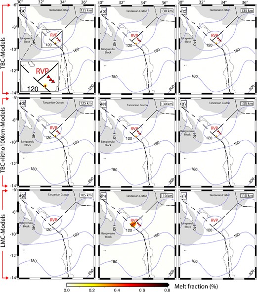
(a), (b) and (c) show depth slices of melt fractions beneath the RVP due to TBC at 125, 130 and 135 km depth, respectively. (d), (e) and (f) show depth slices of melt fractions beneath the RVP due to TBC with a uniform 100-km thick lithosphere (TBC-litho100km) at 125, 130 and 135 km depth, respectively. (g), (h) and (i) show depth slices of melt fractions beneath the RVP due to LMC at 105, 110 and 115 km depth, respectively, which indicate that melt is generated only at 110 km depths. Red triangles represent.
3.2 Tomography-based convection
In our numerical model, TBC in the sublithospheric mantle arises from our temperature conditions. The lithosphere, which is made rigid in the model by imposing a high viscosity (1023 Pa.s), is not deforming. We assume a rigid lithosphere so we can better investigate the sublithospheric mantle flow patterns and determine if there is sublithospheric melt beneath the RVP at present. In order to improve our understanding of the possible origin of the localization of magmatism in the Western Branch of the EAR. We focus our interpretation of the instantaneous TBC for the model with excess temperature in the sublithospheric mantle whose background temperature is constrained with Tp = 1473 K and velocity-density conversion factor of 0.20, which is our preferred model (see Section 3.1.1 and Table 2). Fig. 6(a), (b) and (c) respectively show 150, 200 and 250 km depth slices of sublithospheric mantle flow patterns resulting from our numerical modeling of TBC for our preferred model. Mantle upwelling occurs where there are slow (negative) seismic velocity perturbations (Fig. 2b; Emry et al. 2019) which tend to be slowest at shallower depths beneath the thin lithosphere of the RVP. Sublithospheric mantle downwelling occurs beneath the relatively thick lithosphere of the surrounding cratons. At 150 km depth (Fig. 6a), the sublithospheric mantle upwelling (∼4 cm yr−1) is focused beneath the RVP where the lithosphere is thin (∼100–120 km) with a characteristic radial horizontal mantle flow (∼4 cm yr−1). At 200 km depth (Fig. 6b), the sublithospheric mantle upwelling (∼5 cm yr−1) remains focused beneath the RVP and the horizontal flow pattern (∼3 cm yr−1) is characterized by a southwestward flow between and around the thick cratonic keels of the Tanzanian and Bangweulu Cratons to the base of the lithosphere beneath the Malawi Rift. The horizontal mantle flow stagnates beneath the RVP where there is rapid mantle upwelling (∼5 cm yr−1). At 250 km depth (Fig. 6c) there is a zone of mantle upwelling (∼1 cm yr−1) at the southwestern margin of the Tanzanian Craton, that extends southeastward through the RVP to the northern segment of the Malawi Rift. This mantle flow pattern is consistent with earlier interpretations from seismic studies by Grijalva et al. (2018) and numerical modeling by Koptev et al. (2018).
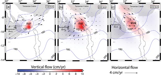
Depth slices showing TBC beneath the RVP and surrounding at (a) 150 km, (b) 200 km and (c) 250 km depth for our preferred model, which is the model with excess temperature in the sublithospheric mantle whose background temperature is constrained with mantle potential temperature, Tp= 1473 K and a velocity-density conversion factor of 0.20. The vertical flow (background colors) is overlain by the horizontal flow field (black arrows). White triangles represent the RVP. Blue contours show lines of equal lithospheric thickness at 20 km intervals from Fishwick (2010). Black lines indicate the outline of rift lakes.
4 DISCUSSION
4.1 TBC versus LMC
In order to better understand the influence of upper mantle heterogeneities and lithospheric thickness variations on sublithospheric mantle flow beneath the RVP and their control on melt localization, we compare mantle flow patterns from the three model groups: (1) TBC, which is TBC model that includes sublithospheric heterogeneities derived from shear wave velocity perturbations (Emry et al. 2019) beneath a rigid lithosphere with laterally variations in thickness (Fishwick 2010; Fig. 7a, b and c); (2) TBC-litho100km, which is a TBC model with sublithospheric heterogeneities beneath a uniform 100-km thick rigid lithosphere (Fig. 7d, e and f); and (3) LMC, which is LMC model driven by lateral variations in lithospheric thickness from Fishwick (2010) and do not include sublithospheric heterogeneities (Fig. 7g, h and i).
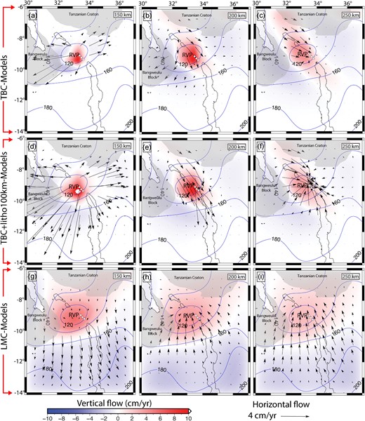
(a), (b) and (c) show depth slices of sublithospheric mantle flow from TBC beneath the RVP at 150, 200 and 250 km depth, respectively. (d), (e) and (f) show depth slices of sublithospheric mantle flow beneath the RVP due to TBC with a uniform 100-km thick lithosphere (TBC-litho100km) at 150, 200 and 250 km depth, respectively. (g), (h) and (i) show depth slices of sublithospheric mantle flow beneath the RVP due to LMC at 150, 200 and 250 km depth, respectively. The vertical flow (background colors) is overlain by the horizontal flow field (black arrows). White triangles represent the RVP. Blue contours show lines of equal lithospheric thickness at 20-km intervals from Fishwick (2010). Black lines indicate the outline of rift lakes.
The mantle flow fields from the TBC model (Fig. 7a, b and c) and TBC-litho100km model (Fig. 7d, e and f) are similar, except that the TBC-litho100km model is ∼1.5 times faster owing to the lower overburden pressure exerted by the uniform 100 km thin lithosphere compared to lithospheric thicknesses >110 km beneath the RVP (Fig. 2a). The similarities in the flow fields regardless of whether the lithosphere is flat or varies in thickness suggest that sublithospheric heterogeneities from shear wave velocity perturbations (Emry et al. 2019) exert a dominant control on the upper mantle flow and also the localization of melt beneath the RVP (see Section 3.1.2). At shallow sublithospheric depths (150 km), the TBC model (Fig. 7a) and TBC-litho100km model (Fig. 7d) show a more focused region of upwelling beneath the RVP with a characteristic radiating pattern of horizontal flow compared to the LMC model. The LMC model (Fig. 7g) shows a broad zone of upwelling beneath the thin lithosphere of the RVP and a general southward horizontal flow beneath the thick lithosphere in the southern parts of the Malawi Rift. At deeper depths (200 and 250 km), the return horizontal mantle flow from the LMC model (Fig. 7h and i) comes from the south and flow northward towards the upwelling region beneath the RVP (Fig. 7h and i), while in the TBC model (Fig. 7b and c) and TBC-litho100km model (Fig. 7d and e) the horizontal mantle flow fields originate from the southwestern part of the Tanzanian Craton and flow southward towards the upwelling region beneath the RVP.
Fig. 8(a), (b) and (c) respectively show depth sections of the TBC, TBC-litho100km and LMC models with melt generation beneath the RVP along profile AA′. And similarly, the TBC, TBC-litho100km and LMC models with melt generation beneath the RVP along profile BB′ are respectively shown in Fig. 8(d), (e) and (f). The main novelty of this work is that the TBC model (Fig. 8a and d) and TBC-litho100km model (Fig. 8b and e), which have constraints on the upper mantle structure from upper mantle velocity perturbations (Emry et al. 2019), show mantle flow patterns that are not evident in the LMC model (Fig. 8c and f). For example, the TBC model (Fig. 8a and d) and the TBC-litho100km model (Fig. 8b and e) show two regions of mantle upwelling beneath the Tanzanian Craton, a region of upwelling beneath the southwestern limit of the craton (Fig. 8a and b) and another region of upwelling beneath the southeastern limit of the craton (Fig. 8d and e). The upwelling beneath the southeastern limit of the craton (Fig. 8d and e) is consistent with results from fully coupled thermomechanical models by Koptev et al. (2016, 2018), which suggest a non-uniform splitting of the Kenyan plume underneath the southeastern part of the Tanzanian Craton to synchronously form the Eastern Branch, the Western Branch and the Malawi Rift. Moreover, the upwelling beneath the southerwestern part of the Tanzanian Craton is consistent with findings of kimberlite deposits beneath the Tanzanian Craton and might be the source of the Igwisi Hills Quaternary kimberlites (Dawson 1994). These upwelling features are absent in the LMC model (Fig. 8c and f). The Igwisi Hills volcanoes on the Tanzanian Craton are the youngest known kimberlite bodies with Upper Pleistocene/Holocene eruption ages based on cosmogenic 3He exposure dating of olivine in the lavas and supported by paleomagnetic analysis (Brown et al. 2012). Brown et al. (2012) suggest that such young eruption ages may indicate that the Tanzanian Craton is undergoing a new phase of kimberlitic volcanism and may erupt more kimberlitic magma in the future. The upper mantle structure beneath the Tanzanian Craton is characterized by the presence of low velocity anomalies (Fig. 2b; Emry et al. 2019) which translates to excess temperature and density perturbations (buoyancy forces) that drive upwelling beneath the craton.
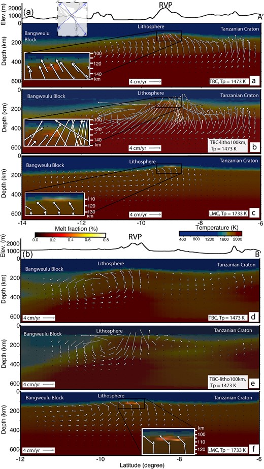
(a) Profile showing present-day TBC and melt generation beneath the RVP (profile AA′; see inset map) for the model with excess temperature in the sublithospheric mantle whose background temperature is constrained with Tp= 1473 K. (b) Profile showing sublithospheric mantle flow due to TBC with a uniform 100-km thick lithosphere (TBC-litho100km) and melt generation beneath the RVP (profile AA′) for the model with excess temperature in the sublithospheric mantle whose background temperature is constrained with Tp = 1473 K. (c) A profile of LMC (model without tomography-based excess temperature in the sublithospheric mantle and the background temperature is constrained with Tp = 1733 K) and melt generation beneath the RVP along profile AA′. (d) Same as (a) but for profile BB′ (see inset map). (e) Same as (b) but for profile BB′. (f) Same as (c) but for profile BB′. The melting regions in Fig. 8(a), (b), (c) and (e) are zoomed-in for better visibility and shown as insets.
The TBC and TBC-litho100 km models along profile BB′ (Fig. 8d and e) reveal a convection cell adjacent to the southeastern margin of the Bangweulu Block that is not evident in the LMC model along profile BB′ (Fig. 8f). This difference may be because the upper mantle constraints (Emry et al. 2019) indicate that the base of the cratonic block is cold and the cratonic block might be thicker than the estimates from Fishwick (2010).
The LMC model, which do not include shear wave velocity constraints (Emry et al. 2019) of sublithospheric heterogeneity (Fig. 8c and f) indicates lateral mantle flow at the LAB over a longer interval than it is in the TBC model (Fig. 8a and d) and in the TBC-litho100km model (Fig. 8b and e). Thus, estimates of mantle tractions (basal drag) from lithosphere-asthenosphere interactions might be overestimated for mantle convection models constrained only by the lithospheric structure (LMC) without considering the upper mantle structure.
4.2 Origin of melt beneath the RVP and the tectonic implications
The most prominent feature in our model is the isolated region of sublithospheric mantle upwelling and localized melt generation due to TBC beneath the RVP at depths of ∼120–140 km. The positive temperature anomalies (∼250K) in the sublithospheric mantle beneath the RVP inferred from shear wave velocity perturbations (Fig. 2b; Emry et al. 2019) suggests the presence of plume material beneath the RVP. The excess temperature of plume material based on petrological studies is ∼200–300 K (i.e. McKenzie & O'Nions 1991; Schilling 1991; Watson & McKenzie 1991; Herzberg & O'Hara 2002; Herzberg et al. 2007; Putirka 2008). Petrological studies by Herzberg & Gazel (2009) suggest excess temperature of ∼100–250 K for hotspots in general. Thus, the low velocity anomaly beneath the RVP may be a consequence of partial melts generated from plume material that is deflected by the cratonic keels of the Tanzanian and Bangweulu Cratons and focuses beneath the thin lithosphere of the RVP as earlier suggested by Grijalva et al. (2018) and Koptev et al. (2018).
Geochemical studies of lava and tephra samples from the RVP by Hilton et al. (2011) show significantly elevated 3He/4He (>15 RA, where RA is the helium isotopic ratio in air), far exceeding typical upper mantle values (generally <9 RA; Graham et al. 2014). Such plume-like 3He/4He ratios, suggest that mantle plume material contributes to the magmatism of the RVP. The high mantle potential temperature (1693–1723 K; Rooney et al. 2012) and excess temperatures of ∼250 K in the sublithospheric mantle beneath the RVP are other indications of hot plume material beneath the RVP. The presence of low shear wave velocity perturbations (Emry et al. 2019) where the lithosphere is thin indicates that the ‘present-day’ sublithospheric melt is a combination of melt from plume materials and decompression melt in response to lithospheric stretching (Yu et al. 2020) assuming that the present lithospheric structure and underlying plume material have not changed significantly in the recent geologic past. A recent review study of the Cenozoic magmatism of East Africa by Rooney (2020) suggests a general shift of magma reservoirs from lithospheric mantle (Type II lavas) to a hybrid of lithospheric mantle and sublithospheric mantle (Type IV lavas) to subsequently sublithospheric mantle (Type III lavas). This shift of magma reservoirs supports our ‘present-day’ observation of sublithospheric melt beneath the RVP.
4.3 Model limitations
Important factors that control the fraction of melt generated in a geodynamic model includes the choice of parametrization for melting, which depends on temperature and pressure and the assumed composition of the source material. We use the parametrization of Katz et al. (2003) for anhydrous peridotite. This parameterization is applicable for pressures less than 13 GPa. Although we use the melting parametrization of anhydrous peridotite (Katz et al. 2003), it has been shown that high water content (Katz et al. 2003) and the use of recycled crustal material (Sobolev et al. 2007, 2011) are also known to enhance melt production by several per cent. Although there might be some uncertainties in the computed melt fractions related to the constraints used for melt generation and the composition of the mantle beneath the RVP, our choice of anhydrous peridotite is appropriate since the RVP is far from any subduction zone that will contribute high water content and recycled crustal materials in the sublithospheric mantle.
A major simplification in this study is the assumption of a rigid lithosphere with a uniform viscosity of the 1023 Pa.s and also the assumption of a linear temperature distribution in the lithosphere; however, the study by Njinju et al. (2019b) suggest significant lateral variations in crustal heat flow beneath the RVP and the Malawi Rift. Moreover, radioactive heat production is higher in the crust than in the lithospheric mantle (e.g. Artemieva & Mooney 2001), thus the lithospheric geotherm should have a higher gradient in the upper crustal part of the lithosphere. The non-linearity in lithospheric geotherm and rheological stratification of the lithosphere play important roles in plume-lithosphere interactions (e.g. Burov 2011; Koptev et al. 2016, 2018, 2021); however, we are not modeling lithospheric deformation and our model setup captures the essential sublithopheric mantle flow patterns beneath the RVP and surroundings.
Another simplification in this study is chemical homogeneity in the upper 660 km of the mantle. We assume the seismic anomalies (Emry et al. 2019) are due to purely thermal effects in an isochemical mantle convection framework. This approach has been successful in numerous previous studies. For example, by representing seismic structures as mantle density and buoyancy structures in a purely thermal, whole mantle convection model, geodynamic studies have not only reproduced the Earth's geoid, but also provided constraints on the mantle viscosity structure (e.g. Hager & Richards 1989). In another case, by assuming thermal large low shear velocity provinces, Lithgow-Berterlloni & Silver (1998) explain dynamic topography signatures which, like the geoid, have two prominent topographic highs over southeast Africa and south Pacific. Despite successful implementations of isochemical mantle convection models, the Earth's mantle is chemically heterogeneous as indicated by a rich variety of geochemical signatures found in mantle derived basalts (i.e. Kunz et al. 1998; Rooney 2020) and from numerically modeling of thermochemical plumes (Dannberg & Sobolev 2015). Thus, the observed low velocity anomaly beneath the RVP (Emry et al. 2019) might also be due to compositional variations in the upper mantle in addition to thermal perturbations. Moreover, the horizontal resolution of the shear wave velocity perturbation (Emry et al. 2019) is ∼1°, thus there is a need for joint-inversions of high-resolution geoscience data sets to better resolve small wavelength features in the upper mantle. However, we show through a vote map (Shephard et al. 2017) that the shear wave velocity perturbations from Emry et al. (2019) compares well with globally available shear wave tomography models in the area (see Fig. S2) with up to 15 shear wave tomography models consistently showing the high velocity perturbation zones in the southern part of the Malawi Rift.
5 CONCLUSIONS
In this study, we develop an instantaneous 3D thermomechanical model of TBC beneath the RVP that incorporates melt generation. We assume an approximately conductive geotherm for the lithosphere, while for the sublithospheric mantle, we use an adiabatic increase in temperature with additional temperature perturbations derived from shear wave seismic velocity constraints. We assume a rigid lithosphere and use non-Newtonian, melt-dependent creep laws of anhydrous peridotite for sublithospheric mantle convection. The seismic constraints indicate excess temperatures of ∼250 K in the sublithospheric mantle beneath the RVP suggesting the presence of a plume. Our TBC simulation is characterized by an isolated sublithospheric mantle upwelling beneath the thin lithosphere of the RVP, which generates melt (∼0.8 per cent melt) at depth of ∼130 km. We test the competing roles of sublithospheric heterogeneities and lithospheric thickness variations in upper mantle convection and find that sublithospheric heterogeneities from shear wave velocity perturbations (Emry et al. 2019) exert a dominant control on upper mantle flow and the localization of melt beneath the RVP regardless of whether the lithosphere is flat or varies in thickness. Results of our TBC reveal some characteristic mantle flow patterns (such as mantle upwelling beneath the Tanzanian Craton and a corner flow adjacent to the southeastern margin of the Bangweulu Block) that are not evident in LMC mantle flow models constrained by lithospheric thickness alone. The LMC model shows lateral mantle flow at the LAB over a longer interval than it is in the TBC models, which suggest that estimates of mantle traction (basal drag) from lithosphere-asthenosphere interactions might be overestimated for mantle convection models constrained only by the lithospheric architector without considering upper mantle heterogeneities. Results from our TBC suggest plume materials are the likely source of deep melt for the RVP which explains the high 3He/4He values in the volcanic materials and the elevated mantle potential temperatures. However, the slowest shear wave velocity perturbations (Emry et al. 2019) occur where the lithosphere is thin, which suggest that the ‘present-day’ sublithospheric melt is a combination of melt from plume materials and decompression melt in response to lithospheric stretching (Yu et al. 2020). We conclude that excess temperature from plume material is necessary for deep melt generation beneath the RVP and possibly beneath other isolated volcanic centers in the Western Branch of the EAR because passive asthenospheric upwelling of ambient mantle will require higher-than-normal mantle potential temperatures to generate melt. Further constraints on lithospheric structure and sublithospheric structure of the upper mantle are required to better understand lithosphere-asthenosphere interactions, deep melt generation and the origin of the localization of magmatism within the magma-poor Western Branch of the EAR.
SUPPORTING INFORMATION
njinju_et_al_2023_GJI_resubmission_supplement_may18.pdf
Please note: Oxford University Press is not responsible for the content or functionality of any supporting materials supplied by the authors. Any queries (other than missing material) should be directed to the corresponding author for the paper.
ACKNOWLEDGEMENTS
This project was supported by the NSF EarthCube Integration grant #1740627. Most of the figures in this paper were generated with Generic Mapping Tools V5.4.2 (Wessel et al. 2013). We also created some of the figures with VISIT v2.9 developed by the Lawrence Livermore National Laboratory. We thank the Computational Infrastructure for Geodynamics for supporting the development of ASPECT, which is funded by National Science Foundation Awards EAR-0949446 and EAR-1550901. Special thanks goes to the Editor Dr. Gael Choblet for handling this manuscript. We would also like to thank Dr. Alexander Koptev and an anonymous reviewer for their helpful comments, which greatly helped to improve this manuscript.
DATA AVAILABILITY
The lithospheric thickness file can be accessed from the BALTO Hyrax server through the URL http://balto.opendap.org/opendap/lithosphere_thickness/. The seismic tomographic model used in this study is available online from the IRIS Earth Model Collaboration (http://ds.iris.edu/ds/products/emc-africaantemry-etal2018/). The mantle flow model output files are available at the Open Science Framework repository with doi: https://doi.org/10.17605/OSF.IO/MZEY9 (Njinju 2023a). The ASPECT code and modified initial temperature, initial composition and material models are available for open access through Zenodo at doi: https://zenodo.org/badge/latestdoi/633193119 (Njinju 2023b).
CONFLICT OF INTEREST
All authors certify that they have no affiliations with or involvement in any organization or entity with any financial interest or non-financial interest in the subject matter or materials discussed in this manuscript.
