


SUMMARY
Türkiye poses a complex crustal structure and tectonic settings owing to the northward convergence of the Arabian and African plates with respect to the Anatolian and Eurasian plates. A reliable 3-D crustal structure of the unruptured segment of the North Anatolian Fault Zone (NAFZ) in the Sea of Marmara is thus of utmost importance for seismic hazard assessments considering that the megacity Istanbul—with more than 15 million habitants—is close to this seismic gap. This study provides high-resolution shear wave velocity images of northwestern Türkiye, including the NAFZ, revealed from ambient seismic noise tomography. We extract over 20 000 Green’s functions from seismic ambient noise cross-correlations and then construct group velocity perturbation maps from the measured group delays with a transdimensional Bayesian tomographic method. We further perform an S-wave velocity inversion to image depth-varying velocity structures. Our high-resolution data allowed us to image S-wave velocities down to 15 km depth and reveal weak crustal zones along the NAFZ, as indicated by low shear wave velocities. We find a low-velocity zone along the Main Marmara Fault, linked with aseismic slip and a deep creep mode. Furthermore, we identify a high-velocity anomaly associated with the unruptured section that defines the boundaries of the locked zone in the crust, which can potentially trigger a destructive earthquake in the future.
1 INTRODUCTION
The convergence of the Arabian and African plates to the Eurasian plate has a dominant control on the evolution of tectonic settings in Anatolia and its adjacent regions (McKenzie 1972). The northward movement of the African plate along the Hellenic trench has led to the slab roll-back response and the extensional regime in western Anatolia (e.g. Taymaz et al. 1991; Confal et al. 2018). The Arabian plate is moving to the north, creating a compressional environment in eastern Anatolia. The difference in gravitational potential energy between these two boundaries leads to the westward flow of the Anatolian lithosphere (England et al. 2016) with shear focused on two major shear deformation zones, the North Anatolian Fault Zone (NAFZ) and the East Anatolian Fault Zone (EAFZ, Fig. 1). The NAFZ, a ∼1600 km long right-lateral transform plate boundary between the Arabian, African and Eurasian plates is one of Türkiye’s most seismically active regions (e.g. Barka 1992). Several devastating historical earthquakes have ruptured about 900 km of its entire length, with an overall westward migrating pattern along the NAFZ (Stein et al. 1997). The first severe failure of the 20th century within our region of focus (red box in Fig. 1) occurred along the Ganos segment located at the westernmost part of the NAFZ in 1912. Two recent destructive earthquakes, the Izmit (Mw 7.4, 1999 August 17) and the Düzce earthquake (Mw 7.2, 1999 November 12), have ruptured the northwestern branch of the NAFZ (see Fig. 2 for the locations of the earthquakes). Historical earthquake records (e.g. Ambraseys & Jackson 2000) reveal that the region between the 1912 and 1999 ruptures forms a seismic gap in the Sea of Marmara (Barka et al. 2002).
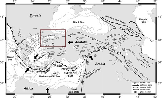
Active tectonics of Anatolian Plate modified after Taymaz et al. (2007) and Yolsal-Çevikbilen et al. (2012). Large black arrows indicate relative plate motions with respect to Eurasia (McClusky et al. 2003; Reilinger et al. 2006). Bathymetric contours are obtained from GEBCO-BODC (1997) and, Smith & Sandwell (1997), and are shown at 500, 1000, 1500, 2000 m. The red rectangle shows the study area. AS: Apseron Sill, BF: Bozova Fault, BGF: Beysehir Gölü Fault, BMG: Büyük Menderes Graben, BuF: Burdur Fault, CTF: Cephalonia Transform Fault, DSF: Dead Sea Transform Fault, DF: Deliler Fault, EAFZ: East Anatolian Fault Zone, EcF: Ecemiş Fault, EF: Elbistan Fault, ESFZ: Ezine Pazarı-Sungurlu Fault Zone, ErF: Erciyes Fault, G: Gökova, Ge: Gediz Graben, GF: Garni Fault, IF: Iğdır Fault, K: Karlıova, KBF: Kavakbaşı Fault, KF: Kagizman Fault, KFZ: Karataş-Osmaniye Fault Zone, MF: Malatya Fault, MRF: Main Recent Fault, MT: Muş Thrust, NAFZ: North Anatolian Fault Zone, NEAF: North East Anatolian Fault, OF: Ovacik Fault, PSF: Pampak-Savan Fault, PTF: Paphos Transform Fault, SaF: Salmas Fault, Si: Simav Graben, SuF: Sultandağ Fault, TeF: Tebriz Fault, TF: Tatarli Fault, TGF: Tuz Gölü Fault and TuF: Tutak Fault.
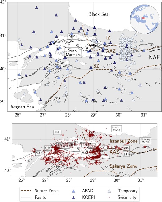
Map of the study area. Top: locations of the seismic stations used in this study. Insert map shows the relative location of the study area. Bottom: t he seismicity around the Sea of Marmara. The seismicity ranges between 0.7–4.5 Mw and is taken from Wollin et al. (2018). AAZ: Armutlu-Almacık Zone, AB: Adapazarı Basin, CB: Central Basin, CH: Central High, ÇIB: Çınarcık Basin, IZ: Istanbul Zone, GI: Gulf of Izmit, GM: Ganos Mountains, GS: Gulf of Saroz, KB: Kumburgaz Basin, MMF: Main Marmara Fault, NAF: North Anatolian Fault, PB: Pamukova Basin, SZ: Sakarya Zone, TB: Tekirdağ Basin, ThB: Thrace Basin and WH: Western High.
Precise locations of microseismicity indicated that the two 1999 earthquakes activated seismicity to the south of Istanbul along the northwest branch of the NAFZ beneath the Sea of Marmara (e.g. Taymaz et al. 2004; Sato et al. 2004; Bohnhoff et al. 2013; Schmittbuhl et al. 2016a) and indicate the depth extent of the NAFZ in the crust. However, the region, particularly around the Sea of Marmara, has inadequate seismic coverage due to the lack of offshore seismic stations (Fig. 2). Therefore, our knowledge of the crustal structure in this part is limited. For instance, a well-established local earthquake tomography approach suffers from poor data resolution due to insufficient ray-path sampling in the offshore area. In comparison, cross-correlated ambient noise, which can be extracted from continuous recordings of seismic stations, can help overcome this problem as they enable a tomographic analysis of the offshore and onshore regions using the surface wave ray paths that traverse the region.
The cross-correlation of the ambient seismic wavefield between two seismic stations yields a waveform that is kinematically similar to the Green’s function (e.g. Nishida 2017). The dispersed surface wave components of the Green’s function are most commonly utilized to estimate subsurface seismic velocity. The first regional ambient noise tomography study of eastern Anatolia found that the NAFZ has a high velocity in the upper crust but has no constant signature for deeper sections (Warren et al. 2013). Later, using the same type of information, Delph et al. (2015) investigated the crustal and uppermost mantle shear wave velocity structure of the Anatolia region and its surroundings. Their results match the tectonic and geological units and agree with Warren et al. (2013). The Rayleigh-wave phase-velocity maps of Anatolia inferred from the ambient noise tomography elucidated isotropic and anisotropic velocity variation that seems to be strongly consistent with the tectonic structures and the style of deformation in the crust and mantle (Legendre et al. 2020). Taylor et al. (2019) analysed auto-correlation of ambient seismic noise data from the stations traversing various accretionary complexes (e.g. Istanbul Zone, Sakarya Zone and Armutlu-Almacık Zone) located at the east of the Sea of Marmara. They found that both the northern and southern branches of the NAFZ are clearly associated with strong gradients in seismic velocity that also denote the boundaries of major tectonic units.
The seismic velocity models from the seismic tomography for the northwestern Anatolian active deformation zone are crucial to constrain the geometry and spatial extent of the faults within the crust and upper mantle. Several geophysical investigations involving seismic velocity and attenuation modelling using either traveltime inversion or waveform data extracted for local/regional earthquake recordings delineated both heterogeneous and anisotropic features in the crust (Saunders et al. 1998; Koulakov et al. 2010; Biryol et al. 2011; Yolsal-Çevikbilen et al. 2012; Fichtner et al. 2013a, b; Çubuk-Sabuncu et al. 2017; Licciardi et al. 2018; Wang et al. 2020). Subregional teleseismic tomography studies performed by Papaleo et al. (2017, 2018) delineated P- and S-wave velocity anomalies for the crust and the uppermost mantle associated with the fault zone. Geoelectrical imaging results based on magnetotelluric data inversions successfully identified crustal structures as they revealed clear transitions between conductive and resistive zones of the NAFZ (e.g. Honkura et al. 2000; Kaya et al. 2009, 2013).
Our main target in this study is to develop a new high-resolution seismic velocity model of the crust that can improve our understanding of the region and enable better estimates of seismic hazards in northwestern Türkiye along the NAFZ. This work does not depend on exploiting earthquake data, which, in many cases, may introduce substantial limitations to the model resolution due to the poor signal quality or the limited number of offshore seismic stations. We use ambient seismic noise recordings acquired across dense seismic arrays and their cross-correlations between station pairs. We conduct a probabilistic Rayleigh-wave tomography in order to estimate group velocity maps at different periods. Then, we invert for shear wave velocity versus depth at every spatial point of the Rayleigh-wave group velocity dispersion estimate using a linear inversion scheme (Herrmann 2013). Employing a Bayesian strategy in the construction of tomographic maps is advantageous for robust interpretations of the models since a prior information on velocity structure is included in terms of a probability density function and the posterior distribution of proposed models provides a statistically rigorous appraisal of model uncertainty.
2 DATA AND SEISMIC NOISE CORRELATIONS
In ambient seismic wavefield methods, every seismometer can act as a source; thus, it does not depend on earthquakes. The cross-correlation of ambient seismic diffuse seismic wavefield between two seismic stations represents the impulse response or the Green’s function associated with the media between these stations (e.g. Lobkis & Weaver 2001; Campillo & Paul 2003). A comprehensive review of the ambient noise techniques can be found in Weaver (2005) and Snieder & Larose (2013). The idea was first applied to ambient seismic noise data by Shapiro & Campillo (2004), and the first tomographic images obtained from the inversion of ambient noise-derived dispersion curves were given in Shapiro et al. (2005) and Sabra et al. (2005). Following these studies, seismic ambient noise imaging has rapidly become a popular imaging tool preferred for passive seismology experiments conducted at different depth scales from very shallow to upper-mantle depths in order to delineate subsurface heterogeneities (Yao et al. 2006; Yang et al. 2007; Lin et al. 2008; Moschetti et al. 2010; Zulfakriza et al. 2013; Mordret et al. 2013; Gao & Shen 2014).
In this study, we use continuous seismic noise recordings of 136 temporary and 84 permanent broad-band and short-period seismic stations in the region (Fig. 2), including the Dense Array for North Anatolia (DANA 2012) seismic network, operating between 2012 and 2013 with a dense coverage. To further increase the station coverage, we used the permanent stations from the Kandilli Observatory and Earthquake Research Institute (KOERI), the Directorate of Disaster Affairs (AFAD) networks and other temporary seismic stations operating at various periods between 2005 and 2017. The interstation spacing within our database varies between 7 and 400 km. The sampling rate of the recordings ranges from 20 to 100 Hz. We applied a zero-phase low-pass filter to each seismic record and downsampled to 10 Hz. We used the recordings from various types of sensors to calculate cross-correlations.
After downsampling the data, we followed the steps proposed by Saygin & Kennett (2010, 2012) to process the noise recordings. The cross-correlation is conducted on the digital waveform data of 300 s time intervals with a 60 s overlap extracted from the continuous recordings. In fact, we normalized the cross-correlations (daily) but did not remove the earthquakes. Once the cross-correlation operation is completed, we stack all of the available traces to generate the final interstation correlogram for each station pair. We obtained approximately 24 000 cross-correlations and performed manual visual identification for every cross-correlation to avoid picking noise or higher mode energy. In Fig. 3, two examples from the retrieved empirical Green’s functions are presented, showing highly coherent arrivals of Rayleigh waves with average group velocities of 2.4 km s−1. A narrow-band Gaussian filter was applied to every Green’s function to measure the group velocities from the arrival times by using multiple filter analysis (Dziewonski et al. 1969) between a period range from 1 to 15 s. All the measured dispersion curves are shown in the Supporting Information (Fig. S1). We limit our measurement range up to 15 s, as the signal-to-noise ratio of Green’s functions reduces significantly for greater periods. We pick each group delay time of Green’s functions manually, where the maximum number of traveltimes achieved in the present work is over 6 000 at period 3 s (Fig. 4).
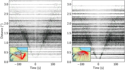
Extracted Green’s functions between all the available stations and TVSB (left), KLYT (right) station. The inset maps indicate the ray paths between stations. All waveforms were filtered between 0.06 and 1.0 Hz and then normalized by absolute unit peak amplitude. Green lines correspond to 2.4 km s−1 group velocity. A gain function with tapering is applied to the cross-correlations to suppress the signal produced by steeply incident teleseismic body waves appearing between −7 and 7 s.
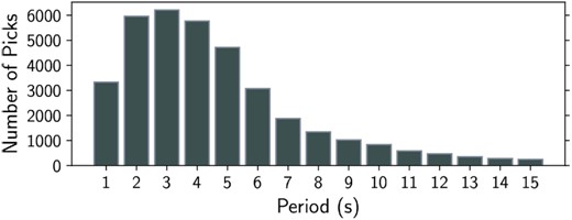
The number of traveltimes that are picked manually for every period between 1 and 15 s. The maximum number of traveltimes is over 6000 for period 3 s.
3 TOMOGRAPHIC INVERSION
After extracting the Green’s functions from seismic ambient noise cross-correlations, we construct the group velocity maps using two different tomographic inversions. First, we applied a simple and computationally fast 2-D nonlinear tomography to gain a first estimate of the group velocity variation in the study area. After, we performed a transdimensional Bayesian inversion on the same data-set. Applying two different inversion schemes helps us to substantiate the two tomographic results. See Rosalia et al. (2020) for a comparison between the subspace and transdimensional inversion.
3.1 Nonlinear inversion
We apply a fully nonlinear 2-D tomographic inversion to the observed traveltimes to produce seismic velocity maps for periods ranging between 1 and 15 s. We use a 0.1° × 0.2° (latitude by longitude) grid spacing and assumed an initial estimate of velocity as 2.4 km s−1 for the inversion at each period. We use the fast-marching method (FMM, Sethian & Popovici 1999; Rawlinson & Sambridge 2004a, b) to achieve forward traveltime calculations and update ray paths at each iteration. The optimum ray paths are updated by applying the fully nonlinear inversion with six iterations. The objective function that is minimized and the regularization parameter are defined by Rawlinson (2007, the choice of regularization parameter is shown in Fig. S4, Supporting Information).
3.2 Transdimensional Bayesian inversion
The transdimensional Bayesian tomography is an approach that allows to obtain an ensemble of solutions with a full probability distribution, allowing a statistical assessment of the model uncertainty (Bodin & Sambridge 2009). The method uses the reversible jump Markov chain Monte Carlo (rj-McMC) method to estimate the probability distribution of the model parameters, as implemented by Bodin & Sambridge (2009). Typical tomographic inversion requires the regularization parameters (e.g. mesh size, damping and smoothing) to be chosen by the user. The transdimensional Bayesian tomography simultaneously inverts for the number of cells in the model, their geometries and their seismic velocities. Thus, the parametrization is directly determined by the data, without the requirement for these subjective choices.
The velocity field is represented with irregular Voronoi cells, which vary in size and shape depending on data resolution conditions in the model space and thus reflect the model resolution due to the irregular distribution of the stations (Sambridge et al. 2013). In order to avoid unrealistic Earth models, the inversion considers a priori information on the parameters, such as the expected range of seismic velocity, the number of cells or the noise level of the observed data. Several transdimensional tomography applications in geosciences have been documented, for instance, to reconstruct the Moho depth variation (e.g. Bodin et al. 2012), to estimate physical properties of the crustal structure (e.g. Saygin & Kennett 2012) beneath Australia, imaging using seismic noise (e.g. Young et al. 2013; Saygin et al. 2016; Kim et al. 2016; Galetti et al. 2017) and transdimensional seismic full-waveform inversion (Visser et al. 2019).
In the present work, we perform the transdimensional Bayesian tomography inversion using the traveltime residuals extracted from the cross-correlated ambient noise data along the northwest of the NAFZ and surrounding regions. For forward modelling, we use the FMM to update the ray paths. For the inversion step, we apply the rj-McMC algorithm (Green 1995) to determine the partitioned velocity models that form the reference model for the next iteration (Bodin & Sambridge 2009). We employ a uniform prior distribution for the group velocity and the number of Voronoi cells ranging between 1.0–3.2 km s−1 and 2–1000 cells, respectively. The rj-McMC was run using 200 parallel Markov chains on a high-performance computer. Each chain was run on a single core and performed 200 000 iterations in total, with 100 000 burn-in steps and 100 000 post-burn-in steps at each period to ensure the convergence. In the first iteration, the ray paths were assumed to be straight lines. Then between each inversion cycle, the ray paths were updated with the new velocity model using the FMM. Five iterations were performed to update the ray-path geometries at each period. The updated velocity models at each iteration for a period of 3 s are shown in Fig. S5 (Supporting Information).
3.3 Resolution tests
An assessment of the reliability of velocity images is required to have an insight into spatial resolution. In particular, for the seismic tomography experiments where it is not possible to make a direct comparison between the models and ground-truth data (e.g. well-log data). We conduct two types of synthetic tests; first, based on a hypothetical structure anticipated for the region and second, based on a checkerboard structure considering the actual ray-path distribution.
We display results from the synthetic data inversion for nonlinear tomography and transdimensional Bayesian tomography (Figs 5b, c, e and f). Besides, we present uncertainty values for the transdimensional Bayesian tomography results at 3 and 10 s (Figs 5d and g). Both methods adequately recover the initial structure for 3 s, although the nonlinear method performs slightly better than the transdimensional one. However, nonlinear tomography depends on the damping and smoothing parameters, introducing bias into the results. When the transdimensional Bayesian tomography is in use, the estimated uncertainty ranges between 0–0.15 km s−1 everywhere except the domain boundaries (Figs 5d and g). For 10 s, even though the ray-path coverage is relatively less dense, both inversions recover the structure reasonably well. In Fig. 5(g), at 10 s, the model uncertainty increases beneath the western part of the study area, where the data resolution is poor due to a lack of high-quality cross-correlations.
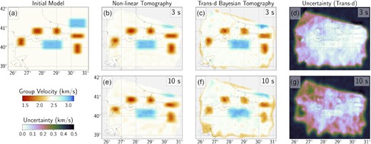
Resolution tests for nonlinear and transdimensional (trans-d) Bayesian inversion. (a) Initial model with 0.1° × 0.2° grid spacing. Estimated model for 3 s period with a maximum ray-path coverage for (b) nonlinear inversion, (c) Bayesian inversion and (d) uncertainty for Bayesian inversion. Estimated model for 10 s period with less ray-path coverage for (e) nonlinear inversion, (f) Bayesian inversion and (g) uncertainty for Bayesian inversion.
A synthetic checkerboard model to test both inversions was performed by dividing the study area into grids with 0.1° × 0.2° spacing with a background velocity of 2.4 km s−1 (Fig. S6, Supporting Information). Gaussian noise with a standard deviation of 0.1 s was added to the calculated synthetic traveltimes. Similar to the synthetic test results described above, the checkerboard test indicates both nonlinear and Bayesian tomography successfully recover the structure at 3 s. At 10 s, however, we are able to resolve the localized velocity anomalies at the right locations for both types of inversions, but a smearing effect is notable on the recovered pattern because of low ray coverage (Figs S6e–g, Supporting Information).
Our sensitivity analyses, overall, suggest that both methods give a good solution when there is a sufficient sampling capacity of the region (i.e. at 3 s). However, probabilistic tomography, in general, has less dependency on user-chosen parameters that are needed for the regularization of the objective function in classical inversion problems. Importantly, transdimensional tomography enables a direct assessment of uncertainties in model parameters that are not readily obtained from the nonlinear inversion. Therefore, we decided to apply Bayesian tomography for further inversion of the observed data to elucidate the crustal structure beneath our study region.
3.4 Shear wave velocity inversion
The dispersion curves at each location in the model are inverted for shear wave velocity versus depth, using a linear inversion scheme using the subroutine surf96 of computer programs in seismology (Herrmann 2013). For each gridpoint, we extracted the group velocities from the transdimensional inversions and applied a gentle smoothing with a four-points running mean to obtain a continuous dispersion curve. A well-known fact of the linearized inversion is that its model solution is dependent on the initial model. To minimize the potential bias caused by an improper choice of model, we constructed an initial model that is representative of the regional 1-D velocity structure by averaging a recent 3-D shear velocity model generated by Delph et al. (2015). To consider the varying data resolution of group velocity inversions, we applied depth-dependent weights to layers in the model. Specifically, we gradually decreased the weight from 1 at 10 km to 0.5 at 20 km, which essentially reduces the deviations from the initial model at greater depths where the spatial resolution is relatively low.
To ensure a smooth model solution, we also applied the smoothness constraint to the inversion. The degree of smoothness is controlled by the damping parameter. The objective function to be minimized is defined by Herrmann & Ammon (2002). We determined the optimal damping value by examining the L-curve that defines the relationship between the inversion misfit and model norm. We constructed an L-curve at each node location by varying the damping value from 0.05 to 10. The optimal damping value corresponds to the turning point of the L-curve where the curvature reaches the maximum (Fig. S10, Supporting Information). It is worth noting that not all node locations are equally well-constrained, and the turning points can be missing or biased at certain locations. In such cases, we adopted the damping values from the nearby inversion nodes where the turning points are clearly defined. Overall, the effect of damping on the final velocity model is only secondary; damping mostly affects the amplitudes of the velocity perturbations while the pattern remains largely stable. The inversion was conducted iteratively, and a total of 10 iterations were performed. An example of data fit and model solution is shown in Supporting Information (Fig. S11). The final 3-D model was obtained by combining 1-D velocity profiles at all node locations.
4 DISCUSSION
Using ambient noise cross-correlations allowed us to obtain good ray-path coverage, resulting in high-resolution velocity images compared to previous seismic tomography studies in the region down to 15 km depth. The application of transdimensional Bayesian tomography offered uncertainty quantification as well as treatment of irregular ray-path coverage in some places. In the uncertainty images, some doughnut-shaped anomalies are notable, generally located in the low-velocity regions. This phenomenon occurs due to the discontinuities in the Voronoi cells (e.g. Galetti et al. 2015; Section 3 in the Supporting Information). Below we show the results from the resolution tests and final velocity images. We further discuss some of the prominent velocity anomalies and interpret them in the light of available constraints on geology, tectonics and the deformation history of the region.
4.1 Comparison of the nonlinear and transdimensional group velocity maps
The group velocity maps obtained by nonlinear tomography (Fig. S7a, Supporting Information) and transdimensional Bayesian tomography (Fig. 6a) show first-order similarities. Most of the distinct velocity anomalies are located at similar locations. However, the anomalies seem to be smeared along ray paths more strongly in nonlinear tomography group velocity images. The smearing effect possibly stems from the fact that the nonlinear tomography inversions for group velocity estimates are more sensitive to the ray-path coverage that decreases with increasing period (e.g. the number of traveltimes in Fig. 4 and the ray-path coverage in Fig. S7b, Supporting Information). The nonlinear inversion is less successful in updating the reference model with the low ray-path coverage compared to the transdimensional inversion (Rosalia et al. 2020). Damping and smoothing parameters can introduce further strong artefacts into the solution. On the other hand, in the transdimensional Bayesian tomography images, the smearing effect is visibly subdued.
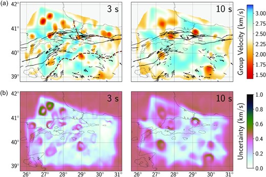
Transdimensional Bayesian inversion results and uncertainty maps. (a) Group velocity images obtained from transdimensional Bayesian tomography for periods 3 and 10 s. The group velocity ranges between 1.4 and 3.2 km s−1. Black lines represent the NAFZ, dashed brown lines represent the suture zones. (b) The uncertainty maps for periods 3 and 10 s. The uncertainty ranges between 0.0–1.0 km s−1.
Another interesting observation is that a shift between specific anomalous features in the group velocity maps obtained by the two inversion methods, for example, a low-velocity anomaly between 28.5°E–28.9°E 40.7°N–40.9°N (at 3 s of Fig. S7a, Supporting Information) appears to be shifted west compared to the one in the 3 s map of Fig. 6(a). This shifting behaviour might be due to the combination of the fixed gridding and smearing effect in nonlinear tomography. The insensitivity of the Bayesian inversion approach to any user-dependent parameters during the regularization of the objective function is the reason in the present work we rely on its resultant group velocity distributions.
4.2 Tectonic units
As a significant tectonic feature within our study area, the NAFZ and its segments are well marked by a number of low-velocity features in the upper 10 km or so (Fig. 6a and Fig. S4a, Supporting Information). These features might be interpreted as zones of highly deformed and distributed crustal features along major fault zones. Full-waveform modelling studies have earlier imaged low velocities aligned with the NAFZ (e.g. Fichtner et al. 2013a, b; Çubuk-Sabuncu et al. 2017). Similar low-velocity features along the NAFZ were also observed in a regional ambient noise tomography experiment (e.g. Delph et al. 2015) and a recent local earthquake tomography study (Wang et al. 2020) covering the entire Anatolia.
East of the Sea of Marmara, the NAFZ crosses different geological zones such as Istanbul Zone, Sakarya Zone and Armutlu–Almacık Zone and splits into two branches (Fig. 2). The southern strand of NAF (SNAF) forms a boundary between Sakarya Zone and Armutlu–Almacık Zone, and the northern strand (NNAF) continues beneath the Sea of Marmara.
The Istanbul Zone is a 400 km long and 55 km wide continental fragment originally belonging to Laurasia with a Precambrian crystalline basement overlaid by a continuous sedimentary sequence (e.g. Yilmaz et al. 1997; Okay & Tüysüz 1999). At the eastern part of the Istanbul Zone, the NAFZ bounds the Adapazarı Basin with its northern branch (40.7°N–30.2°E). Shear wave velocity images shown in Fig. 7 highlight the basin with a low shear velocity at the depths of 2 and 5 km but not at 10 and 15 km depths. This low-velocity zone might also be associated with the earthquakes that happened along the NAFZ within the last century, and thus, Hussain et al. (2016) conclude that it is a locked domain and accumulates strain. A low-velocity anomaly would be expected if there was an aseismic creep domain. Some part of this low-velocity anomaly at shallow depths (1–6 km) ranges might be rather due to the faulted sediments in the northwestern part (Şengör et al. 2005). From depth cross-sections along with profiles CC′ and BB′ (Figs 8 and 9), this low-velocity anomaly can be traced down to 2.5–3 km depth, which likely corresponds to the total sediment thickness of the basin. Similar to our results, Taylor et al. (2019) suggested the sedimentary thickness of the Adapazarı Basin to be around 2.5 km.

The S-wave inversion images at 2, 5, 10 and 15 km of depth obtained from inverting the transdimensional Bayesian group velocities. Black lines represent the NAFZ, and dashed brown lines represent the suture zones.
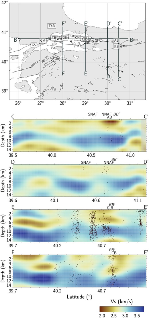
S-wave velocity sections and their locations. The depth ranges between the surface and 15 km. The map indicates the locations of the profiles. Black lines represent the NAFZ. The seismicity (red dots) ranges between 0.7–4.5 Mw and is taken from Wollin et al. (2018). The orthogonal sections are marked on the plots. AB: Adapazarı Basin, CB: Central Basin, ÇIB: Çınarcık Basin, SNAF: Southern branch of the North Anatolian Fault and NNAF: Northern branch of the North Anatolian Fault.
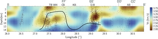
The shear wave velocities along the cross-section BB′. See Fig. 8 for the location of the cross-section. The black line indicates the locking depth extracted from Schmittbuhl et al. (2016b). The seismicity (red dots) ranges between 0.7–4.5 Mw and is taken from Wollin et al. (2018). The orthogonal sections are marked on the plots. AB: Adapazarı Basin, CB: Central Basin, ÇIB: Çınarcık Basin, KB: Kumburgaz Basin, TB: Tekirdağ Basin and WH: Western High.
In the western part of the Istanbul Zone (41.2°N–29°E), we observe significant high-velocities in our group (Fig. 6a), and shear velocity (Fig. 7) maps that match with the presence of Precambrian crystalline basement in the region. At depths greater than 5 km, along with the profile DD′ and EE′, at the higher longitudes (41°N), the shear velocities significantly increase to 3.5 km s−1 or higher. Teleseismic P- and S-wave tomography images presented in Papaleo et al. (2017, 2018) confirm similar high-velocity anomalies that can be attributed to the dominant effect of Precambrian crystalline rocks. Armutlu-Almacık Zone is located between two strands of the NAFZ on the east margin of the Sea of Marmara (e.g. Fig. 1). Armutlu Block, bounded between the Istanbul and Sakarya zones, has a high topography being the continuation of the Armutlu Mountains. It consists of different metamorphic rocks, which are a melange of the Istanbul and Sakarya zones. Our group velocity maps identified the Armutlu–Almacık Zone by relatively high-velocity estimates with low uncertainties of model parameters (ranging from 0.0 to 0.3 km s−1). The high-velocity anomaly is due to the presence of high-density metamorphic rocks (e.g. Okay & Tüysüz 1999). Taylor et al. (2019) observed relatively high S-wave velocities within the Armutlu–Almacık Zone. Another significant anomaly is located in the southeastern part of the Armutlu–Almacık Zone, coincident with the Pamukova Basin which, like the Sakarya Basin, is a pull-apart basin at a point where the fault is oblique to the relative motion vector. In our Vs images (Fig. S9, Supporting Information, the cross-section ZZ′), the area where Pamukova Basin is located exhibits low velocities at a depth of 2–2.5 km, and while at deeper parts, high shear wave speeds become prominent. Similarly, Taylor et al. (2019) proposed a 2.5 km depth for Pamukova Basin from their surface wave observations.
A drastic change of velocity between the eastern and western part of the Armutlu–Almacık Zone is visible at the longer periods. In Fig. 8, the cross-section along profile DD′ shows two high-velocity blocks at 10 km depth which might represent the metamorphic rocks of the Istanbul Zone and the Sakarya Zone. The Armutlu–Almacık Zone is located in between those anomalies and marked with a relatively low-velocity anomaly. With the profile CC′, those high-velocity blocks appear to merge, consistent with the rhomboid Armutlu–Almacık block as outlined by the major fault strands. Similar to our results, previous ambient noise and teleseismic tomography works (e.g. Taylor et al. 2019; Papaleo et al. 2017, 2018) were able to detect the high- and low-phase velocity character of the Armutlu–Almacık Zone and Pamukova Basin, respectively. Analysis of P-to-S converted waves from teleseismic sources to model isotropic crustal velocities by Kahraman et al. (2015) found a low-velocity zone beneath Armutlu–Almacık Zone. Besides, modelling coda wave envelopes extracted from local earthquakes (e.g. Izgi et al. 2020) exhibited low attenuation concerning inelastic absorption and scattering properties in this region in accordance with the relatively high group velocities resolved by our Bayesian and nonlinear inversions.
The northwest boundary of the Sea of Marmara hosts a 9 km thick triangular-shaped sedimentary Thrace Basin. This basin is from the Eocene–Oligocene age (e.g. Turgut et al. 1991) and overlies a basement of the Strandja Massif’s metamorphic rocks (Alaygut 1995; Yilmaz et al. 1997). To the south, the Thrace Basin extends beneath the Marmara Sea. Our inversion results identify this thick sedimentary basin with a persistent distribution of low S-wave velocity as similarly observed in other basins of the study area (Fig. 7). We can trace the basin down to 9–10 km depths. At depths greater than 10 km, a significant high-velocity anomaly can be attributed to the presence of high-grade metamorphic rocks (Görür & Okay 1996) at the northeast of the basin. The concentration of low shear wave speeds in the sediments of the basin can also be related to the presence of gas. Gürgey (2015) successfully map the localities of oil and condensate-wet gas at depths below 3.6 km, estimating more than 1.15 per cent volume of basin sediments in the form of condensate gas. The low-velocity zone beneath the Thrace Basin tends to match well with prospective oil and gas locations and could potentially explain modelled low velocities down to 10 km depth in the S-wave velocity maps (Fig. 7). Similar to Yilmaz et al. (2016), the location of oil and gas fields in the Thrace Basin matches our low-velocity zones.
4.3 Structure beneath the Sea of Marmara
The NAFZ bifurcates into shorter segments and is discontinuous while it further continues to the west (Barka & Kadinsky-Cade 1988). It crosses the Sea of Marmara within a 280 km long and 80 km wide marine basin. It is represented by several complex structures developed within a zone of interaction between the extensional and the strike-slip shear deformation regimes (e.g. Gürer et al. 2006). The three segments beneath the Sea of Marmara are; the 15 km long Ganos segment, which could have broken during the 1912 earthquake (e.g. Ambraseys & Finkel 1987); the 105 km long Central Marmara Segment representing a seismic gap since 1766 (e.g. Okay et al. 2000); and the 45 km long North Boundary segment which failed during the 1894 rupture (e.g. Ambraseys & Finkel 1987). Coulomb stress change calculations (e.g. King et al. 2001; Durand et al. 2013) performed following the 1999 Mw 7.4 Izmit earthquake show that the area of new stress accumulation is focusing on this western branch in the Sea of Marmara where a future large earthquake is expected to occur (Bohnhoff et al. 2013).
The NAFZ enters the Sea of Marmara from the Gulf of Izmit as a single strand, continues through the north of the Çınarcık Basin as a bending fault segment and then turns to the east–west direction (Le Pichon et al. 2001). The Çınarcık Basin is a 50 km long and 18 km wide structure with an average water depth of 1270 m (Carton et al. 2007, see Fig. 9 for relative locations). The southern part of the basin represents an extensional field, and farther to the west of this field, the structures consisting of thrust faults and folds form the boundary between the Central High and the Çınarcık Basin (Le Pichon et al. 2001). Early seismic images from wide-angle seismic reflection and refraction profiles in the Sea of Marmara have implied a thinning of the crust under the deep Central Basin that has likely occurred due to extension (Laigle et al. 2008; Bécel et al. 2009, 2010).
Within our tomograms, the Çınarcık Basin is characterized by pervasive low velocities (Fig. 7), ∼2.3 km s−1 of consistent low-velocity block noticeable at depths of 2 and 5 km from our S-wave inversion results are typical for this basin structure. This depth range is consistent with the one elucidated from controlled-source seismic data analyses by Carton et al. (2007), where 5–6 km sedimentary thickness with an average velocity of 2.5 km s−1 was reported for the same basin. However, this low-velocity zone is observed more strongly along the North Boundary segment, which bounds the Çınarcık Basin. From Fig. 8, the cross-section EE′, we recover low-velocity features down to 10 km (∼40.8°N). This feature might be associated with the Çınarcık Basin or the northern branch of NAFZ. Like the North Boundary segment, the Central Marmara segment, is observable with a relatively high S-wave velocity down to a depth of 15 km. The low-velocity block at this depth along this segment is also related to the Central Basin with a spindle-shaped fault zone that continues as a single strand through the Western High (Le Pichon et al. 2001). Our apparent higher absolute group velocities (Fig. 6a) in between the Tekirdağ and Çınarcık basins for periods 1–10 s are consistent with high-velocity P-wave speeds previously reported by Bayrakci et al. (2013) as well as with high resistivity anomalies reported by Kaya (2012) that were attributed to the existing asperity zones in the Sea of Marmara.
The Tekirdağ Basin is the third deep basin of the Sea of Marmara, spindle-shaped and is bounded by the Ganos and Strandja Mountains in the west. Another notable low-velocity region appearing at the western side of the Sea of Marmara in our tomographic images might be associated with the Tekirdağ Basin (Fig. 7). Low velocities in this basin were implied in early studies (e.g. Delph et al. 2015; Çubuk-Sabuncu et al. 2017) but with relatively low-resolution capability compared to our new models. Here we provide valuable constraints on the structure of the Tekirdağ Basin. In Fig. 9, from the depth section along with profile BB′, we are able to recover the low-velocity structure down to about 3 km depth. This low-velocity feature corresponds to the southern border of the Tekirdağ Basin, corresponding to 27.8°E. However, this low velocity continues to the east and connects with the Central Basin. Our findings support the idea of Bayrakci et al. (2013), who claim that the Tekirdağ and Central Basins appear to be linked, forming a 60-km-long basement depression.
4.4 Vertical extents of deep creep and locked zones beneath the Sea of Marmara
The existing seismic gap of ∼150 km unruptured Main Marmara Fault segment (the combination of North Boundary and Central Marmara segment) of the NAFZ beneath the Sea of Marmara has been subject to several studies mainly involving spatio-temporal microseismicity characteristics (e.g. Sato et al. 2004; Bohnhoff et al. 2013; Schmittbuhl et al. 2016b; Wollin et al. 2018). From the seismic hazard assessment perspective, an understanding of whether the accumulated strain energy is being released with large earthquakes along the locked fault or some part of tectonic loading is relaxed in a creeping mode that results in an aseismic behaviour is of utmost importance. Seismological b-value variation (e.g. relatively low and high b-values in the west beneath Central and Çınarcık Basin, respectively) reported in Schmittbuhl et al. (2016b) implied that the creeping fault in the west might change to potentially seismogenic towards the east of the Main Marmara Fault. Early geodetic data analyses in Ergintav et al. (2014) implied such a creeping segment would be active beneath the central part of the Main Marmara Fault starting from ∼3 km below a locked zone. Schmittbuhl et al. (2016b) further observed that the seismicity distribution (depths between 5–15 km) detected for the structures beneath the Tekirdağ and Central basins favoured deep creep behaviour. However, they found the presence of a locked fault segment beneath the Kumburgaz and Çınarcık basins (for more details, see Fig. 7 in Schmittbuhl et al. 2016b). More recently, depending on the observations of sparse seismicity, Wollin et al. (2018) suggested two aseismic zones; beneath the Tekirdağ and Kumburgaz basins extending down to a depth of ∼10 and ∼15 km, respectively. A vertical cross-section along the E-W trending profile B-B′ extracted from our final tomographic model (Fig. 9) presents a profound low-velocity zone between 5 and 12 km depths beneath the Tekirdağ and Central Basin. This zone can be associated with aseismic slip of a deep creep mode as earlier proposed by Schmittbuhl et al. (2016b). Fig. 9 depicts the locking depth boundary (marked by the black line) extracted from the results in Schmittbuhl et al. (2016b) by highlighting a correlation between seismic velocity and microseismic activity in the first 15 km of the crust.
Beneath the fault segment within the Kumburgaz Basin (Fig. 9), a distinct high-velocity region identified with very low seismicity seems to cause a termination of the low-velocity zones located between the Tekirdağ, Central and Çınarcık basins. This part of the NAFZ represents a major seismic gap (Schmittbuhl et al. 2016b). The high-velocity anomaly to the south of this unruptured segment appears coincident with the boundaries of the locked zone in the crust. The accumulated strain in this locked zone can cause a devastating earthquake with Mw7.3 (Schmittbuhl et al. 2016b) considering its present geometry depicted by the high-resolution locations of seismicity. The locked zones are characterized by a thin fault gouge and insignificant rock damage (e.g. Mooney & Ginzburg 1986) that can explain the relatively high-velocity we find in this region. The magnitude estimate depends on the assumption that the rupture will not enter significantly within creeping domains. Schmittbuhl et al. (2016b) suggested a potential supershear in which rupture propagating at velocities greater than S-wave velocities of the surrounding crustal structure could happen in this region due to insignificant stress variations accompanied with very small seismic activity. This type of rupture has been observed for several large earthquakes associated with strike-slip faults (e.g. the 1999 with Mw 7.6 in Izmit, Türkiye, 2001 Mw 7.8 Kunlun, Tibet earthquake, 2002 Mw 7.9 Denali, Alaska earthquake, see Das 2015,and references therein). Supershear rupture has been earlier detected to the east of the NAFZ following modelling of seismo-geodetic data collected during the 1999 Mw7.6 Izmit and Mw7.2 Düzce failures (e.g. Bouchon et al. 2010; Konca et al. 2010). Models and observations from several supershear events have implied that rather straight, and long strike-slip fault segments along a medium with low fault friction and without any other impediments or barriers can generate supershear rupture over significant distances (e.g. Das 2015). Thus, the North Boundary segment within the Central Basin with a low-velocity upper crust can be a potential zone of bi-lateral supershear rupture, particularly considering that the rupture of the main shock will exploit the low-velocity zones within the upper crust.
At the eastern shear zone of the Sea of Marmara, the North Boundary segment of the NAFZ within the Çınarcık Basin exhibits a seismic gap based on precise locations of microseismic activity (e.g. Bohnhoff et al. 2013) and confirmed by geodetic locking depth estimates (Ergintav et al. 2014). Recently, Tarancıoğlu et al. (2020) revealed the high-velocity structure between 6–10 km depths of this relatively small-sized gap compared to the one below the Kumburgaz Basin. Unlike Tarancıoğlu et al. (2020), we resolve relatively high Vs with very low magnitude down to 6–10 km beneath the Çınarcık Basin. Our tomographic models derived from the inversion of ambient noise-based traveltime residuals are more sensitive to ∼3–4 km of sediment infill (e.g. Carton et al. 2007) and rather emphasize its dominant character by masking an expected high-velocity block beneath the basin. Two recent tomographic studies (e.g. Tarancıoğlu et al. 2020, and this study) introduce new constraints on 3-D crustal seismic P- and S-wave speeds that can further enhance our understanding of various seismogenic zones and relevant deformation styles and rheology along the northwest edge of the NAFZ. The observed differences between the two models can be attributed to their resolution capabilities, depending on the utilized data types and modelling approaches.
5 CONCLUSION
We established a Rayleigh-wave empirical Green’s function database via correlations of seismic ambient noise along the northwestern part of Anatolia. Our study region included the Sea of Marmara and three tectonic units separated by branches of the NAFZ. Ambient noise-based imaging is advantageous in places where local seismic activity is absent or is challenging to deploy seismic stations (such as the ocean floor).
To get a first estimate of group velocity variations in the study region, we performed a 2-D nonlinear tomography inversion. We further applied transdimensional Bayesian inversion on the same data set and performed an S-wave velocity inversion. Our results provide a higher resolution model of the group velocity and S-wave velocity variations (to 15 km depth) compared to previous studies in the area. Resulting images of shear velocity variation exhibited low velocities in the upper 3–5 km, typical for basin structures such as, Çınarcık, Tekirdağ and Adapazarı Basins.
Low S-wave velocities mark a clear signature of the NAFZ as an active continental fault zone in the area. We found a low-velocity zone along the Main Marmara Fault related to aseismic slip with a deep creep mode. Furthermore, we detected a high-velocity anomaly linked with the unruptured segment of the crust that defines the lateral limits of the locked zone, which has the potential to cause a catastrophic earthquake (Irmak et al. 2021). We propose that the Central Marmara segment and the North Boundary segment can be potential zones for initiation of propagation in case of a supershear rupture.
SUPPORTING INFORMATION
Figure S1. Rayleigh-waves group velocity dispersion curves measured from the cross-correlation of ambient noise for all station pairs. In this figure, there are 6670 measured Rayleigh-wave dispersion curves.
Figure S2. Cross-spectral beamforming analysis between 0.05–1.0 Hz using two different station network arrays: the KO network that has a broad coverage around our study area and the YH network that has a dense coverage in a smaller area. The subarrays used in the beamforming are shown in the map with triangles. Dark blue triangles indicate the KO network, and dark red triangles the YH network.
Figure S3. Extracted Green’s functions between all the available stations and RKY (left), SPNC (right) station. The inset maps indicate the ray paths between stations. Green lines correspond to 2.4 km s−1 group velocity. A gain function with tapering is applied to the cross-correlations to suppress the signal produced by steeply incident teleseismic body waves appearing between −7 and 7 s.
Figure S4. Effects of different damping (ϵ) and smoothing (η) parameters on the nonlinear inversion results. Please see Herrmann (2013) for the details on damping and smoothing parameters.
Figure S5. Group velocity models obtained from transdimensional Bayesian tomography at each iteration for the period of 3 s which has the maximum ray-path coverage.
Figure S6. Checkerboard tests for nonlinear and Bayesian inversion, (a) initial model for 0.1° × 0.2° grid spacing, (b) estimated model for 3 s period with a maximum ray-path coverage for nonlinear inversion, Bayesian inversion and uncertainty, respectively and (c) 10 s period with less ray-path coverage for nonlinear inversion, Bayesian inversion and uncertainty, respectively.
Figure S7. (a) Group velocity images obtained from 2-D nonlinear tomographic inversion for periods 1, 3, 7 and 10 s. The group velocity ranges between 1.4 and 3.2 km s−1. Black lines represent the NAFZ, and dashed red lines represent the suture zones. (b) The ray-path coverage for periods 1, 3, 7 and 10 s. The dark blue triangles indicate the seismic stations and the black lines show the rays between station pairs.
Figure S8. Transdimensional Bayesian inversion results and uncertainty maps. (a) Group velocity images obtained from transdimensional Bayesian tomography for periods 1, 3, 7 and 10 s. The group velocity ranges between 1.4 and 3.2 km s−1. Black lines represent the NAFZ, and dashed red lines represent the suture zones. (b) The uncertainty maps for periods 1, 3, 7 and 10 s. The uncertainty ranges between 0.0–1.0 km s−1.
Figure S9. Vertical S-wave velocity profiles and their locations. The depth ranges between the surface and 15 km. The map indicates the locations of the profiles and the white area in the map shows the masked area with high resolution. Black lines represent the NAFZ. The seismicity (red dots) ranges between 0.7–4.5 Mw and is taken from Wollin et al. (2018).
Figure S10. The L-curve of the data misfit against the model norm as a function of the damping parameter. The value 0.29 corresponds to the point of maximum curvature.
Figure S11. An example of datafit and model solution for the node 800. Left: shear wave velocity change with depth for one node. Right: Rayleigh-wave velocity for each period shown with black triangles, and the datafit with red line.
Please note: Oxford University Press is not responsible for the content or functionality of any supporting materials supplied by the authors. Any queries (other than missing material) should be directed to the corresponding author for the paper.
Acknowledgement
This is an outcome of a master thesis by Buse Turunçtur at the Graduate School of Istanbul Technical University (Türkiye) supervised by Tuna Eken. We are grateful to Yang Lu, Derek Schutt, and the editor, Huajian Yao, for their valuable comments and suggestions that greatly helped in improving the manuscript. BT acknowledges financial support from Australian National University (ANU) and CSIRO Deep Earth Imaging, Future Science Platform. BT thanks Shubham Agrawal and Matthias Scheiter for their helpful comments on this paper, as well as Malcolm Sambridge and Andrew Valentine for their support. This research was undertaken with the assistance of the resources provided at CSIRO HPC facilities. TE and TT acknowledge financial support from Alexander von Humboldt Foundation (AvH) towards computational and peripheral resources. The facilities of IRIS Data Services, and specifically the IRIS Data Management Center, were used for access to waveforms, related metadata, and/or derived products used in this study. IRIS Data Services are funded through the Seismological Facilities for the Advancement of Geoscience and EarthScope (SAGE) Proposal of the National Science Foundation under Cooperative Agreement EAR-1261681. The other seismic data sets used in this study were obtained from the repositories of KOERI (KO), AFAD (TU), RESIF (http://dx.doi.org/10.15778/RESIF.XW2007, http://dx.doi.org/10.15778/RESIF.YI2008) and The Dense Array for North Anatolia (DANA 2012). We use inversion and FMM of Rawlinson & Sambridge (2004b) in the linear tomography. This study makes use of the computer package rj-tomo, which was made available with support from the Inversion Laboratory (ilab). Ilab is a program for the construction and distribution of data inference software in the geosciences supported by AuScope Ltd, a non-profit organization for Earth Science infrastructure funded by the Australian Federal Government. We use the Scientific Color-Map of F. Crameri (http://www.fabiocrameri.ch). For performing the beamforming, we used the python code from Geophydog (https://github.com/geophydog/Beamforming_in_frequency_domain).
DATA AVAILABILITY
The final velocity model and the dispersion data underlying this paper are available in Zenodo, at https://doi.org/10.5281/zenodo.7645202 (Turunctur et al. 2023). The seismic datasets used in this study are available in the repositories of KOERI at https://www.fdsn.org/networks/detail/KO/, AFAD at https://tdvms.afad.gov.tr/continuous_data, RESIF at http://dx.doi.org/10.15778/RESIF.XW2007, http://dx.doi.org/10.15778/RESIF.YI2008) and DANA at https://doi.org/10.7914/SN/YH_2012 (DANA 2012).
