


SUMMARY
Airborne electromagnetic (AEM) method detects the subsurface electrical resistivity structure by inverting the measured electromagnetic field. AEM data inversion is extremely time-consuming when huge volumes of observational data are involved. Forward modelling is an essential part and represents a large proportion of computational cost in the inversion process. In this study, we develop an AEM simulator using deep learning as a computationally efficient alternative to accelerate 1-D forward modelling. Inspired by Google's neural machine translation, our AEM simulator adopts the long short-term memory (LSTM) modules with an encoder–decoder structure, combining the advantages in time-series regression and feature extraction. The well-trained LSTM network describes directly the mapping relationship between resistivity models with transceiver altitudes and time-domain AEM signals. The prediction results of the test set show that 95 per cent of the relative errors at most sampling points fall in the range of ±5 per cent, with average values within the range of ±0.5 per cent, indicating an overall prediction accuracy. We investigate the effects of the distributions of both resistivity and transceiver altitude in the training set on the prediction accuracy. The LSTM-based AEM simulator can effectively handle the resistivity characteristics involved in the training set and yields great sensitivity to the variations of transceiver altitudes. We also examine the adaptability of our AEM simulator for discontinuous resistivity variations. Synthetic tests indicate that the application effect of the AEM simulator relies on the completeness of the training samples and suggest that enriching the sample diversity is necessary to ensure the prediction accuracy, in cases of observation environments dominated by extreme transceiver altitudes or under-represented geological features. Furthermore, we discuss the influence of network configuration on its accuracy and computational efficiency. Our simulator can deliver ∼13 600 1-D forward modelling calculations within 1 s, which significantly improves the simulation efficiency of AEM data.
1 INTRODUCTION
Airborne electromagnetic (AEM) method is used to detect the variations of electrical properties beneath the Earth's surface by transmitting emission currents and measuring the induced electromagnetic field during flight (Fitterman 2015). Due to the advantages of terrain adaptability and operation efficiency, AEM technology has been used extensively in various applications including mineral exploration (Guo et al. 2020; Koné et al. 2021), groundwater investigation (Delsman et al. 2018; Siemon et al. 2019; Ball et al. 2020; Chandra et al. 2021), environmental monitoring (Dumont et al. 2019; Minsley et al. 2021) and geological mapping (Ley-Cooper et al. 2020; Christensen et al. 2021; Dumont et al. 2021; Finn et al. 2022). Since a typical AEM survey involves sounding locations on the order of 104–107 (Minsley et al. 2021), fast AEM data inversion is a challenge, even though 1-D model parametrization is universally adopted in practical applications.
Forward modelling is a critical part of the inversion process and represents the majority of the computational cost. In conventional inversion cases, forward modelling is performed repeatedly to simulate the physical process in the proposed model and evaluate the residuals of model predictions (Ellis & Oldenburg 1994; Zhdanov 2015). Owing to the huge amount of data, conventional techniques usually take several days to complete data inversion for an AEM survey on distributed computing facilities. Moreover, uncertainty evaluation can be extremely costly (Sen & Stoffa 1996, 2013). For example, Bayesian sampling methods require 105–106 forward modellings to obtain the posterior probability distribution of resistivity for a single AEM sounding observation (Hansen 2021), and the computational cost grows proportionally with the number of sounding locations. Therefore, assessments for model uncertainties are often neglected in practical applications, leading to the possibility of misinterpretation of the underground structure.
Nowadays, deep-learning techniques are increasingly used in AEM data inversion to aid our understanding of the subsurface structure (Noh et al. 2019; Bai et al. 2020; Li et al. 2020; Wu et al. 2021a, 2022a, b; Ji et al. 2022). Most deep learning-based inversion algorithms are data-driven and extract the intrinsic relationship between AEM responses and the underground physical properties from a large training data set. Advanced methods tend to incorporate physical constraints into deep-learning construction (Jin et al. 2020; Karniadakis et al. 2021), potentially accelerating network convergence and enhancing the inversion performance (Asif et al. 2022). The physical constraints are generally embedded in a composite loss function, which is composed of both a model misfit and a corresponding data misfit representing the difference between the model-predicted response and the actual signal (Sun et al. 2021). However, due to the huge number of training samples, computing the data misfits requires a huge number of forward modellings and significantly slows down the network training.
As the most computationally intensive part of the inversion process, forward modelling is critical to the efficiency of AEM data inversion. Conventional 1-D forward modelling for time-domain AEM signals generally contains two steps (Hohmann 1988). The response is first calculated in the frequency domain using kernel functions solved by the Hankel transform (Christensen 1990); then, the time-domain response is obtained by an inverse Fourier transform. Although simulation for a single AEM response takes only about 0.2 s on a common laptop (Li et al. 2016; Li & Huang 2018) and the required massive AEM simulations can be further accelerated by parallel processing (Auken et al. 2015), the total computational cost is multiplied by the number of sounding locations along the AEM flight path and quite expensive. Since deep learning-based algorithms are naturally suited for parallelization and non-linear regression (LeCun et al. 2015), we propose a deep learning-based simulator as an alternative for time-domain predictions of AEM signals to speed up the forward modelling part of the inversion process.
Deep learning has been successfully applied to forward modelling of ground-based time-domain electromagnetics (TEM, Bording et al. 2021). Unlike ground-based measurements, the transceiver altitude in an AEM survey needs to be taken into account as it varies during data acquisition and thus affects the AEM signal. In addition, time-domain AEM signals are dominated by electrical properties of the underground medium (Nabighian & Macnae 1991). The shallow subsurface structure is reflected in the early-time signals, while the deeper medium mainly affects the late-time signals. Therefore, we introduce the long short-term memory (LSTM) network (Hochreiter & Schmidhuber 1997; Gers et al. 2000) because of its impressive capacity for time-series analysis. In contrast to the well-known convolutional neural network, the LSTM network is able to utilize effectively the temporal information with the cyclic connection and gating mechanisms and has achieved great success in applications involving sequential data (Yu et al. 2019), including speech recognition (Graves et al. 2013; Han et al. 2017), intelligent translation (Wu et al. 2016; McCann et al. 2017), TEM data de-noising (Wu et al. 2021b) and time-domain AEM data inversion (Wu et al. 2022a). The higher accuracy for time-series prediction achieved by LSTM networks compared to other deep learning architectures has been demonstrated by Lara-Benítez et al. (2021). Inspired by Google's neural machine translation (GNMT) system (Wu et al. 2016), we establish an LSTM network with an encoder–decoder structure (Vincent et al. 2010), combining the advantages in sequence regression and feature reconstruction. With the incorporation of transceiver altitude, our proposed LSTM network directly translates the subsurface resistivity distributions into AEM responses. The overall goal is to achieve faster forward modellings, hence physical constraints can be incorporated in an accelerated deep learning-based inversion, with the capability of uncertainty evaluation for the resulting model parameters in a reasonable amount of time.
In this study, we develop the deep learning-based AEM simulator and demonstrate its accuracy and efficiency through synthetic tests. The proposed LSTM network shows great sensitivity to the transceiver altitude. We further discuss the influence of network configuration on the prediction performance, and point out the potential role our proposed approach of deep learning-based forward simulations can play in geophysics applications in the future.
2 METHODOLOGY
2.1 LSTM network architecture
Our goal is to develop a forward modelling tool to enable rapid prediction of the time-domain AEM response induced by a given resistivity model. Our AEM simulator for this purpose is based on an implementation of the LSTM network with an encoder–decoder structure, with a subsurface 1-D resistivity model and transceiver altitude as the input and the predicted AEM response as the output.
Our proposed network is mainly constructed by the LSTM cells that are developed from recurrent cells (Gers & Schmidhuber 2000). Each LSTM cell contains a cell state and three gate functions including the input, output and forget gates (Gers et al. 2000). The three gate functions adopt non-linear activation functions and matrix operations, and jointly regulate information flow in the LSTM cell by successively determining the information to be saved or forgotten in the current cell state and to be passed forward to the next cell state. The detailed explanation and corresponding mathematical expressions of the LSTM module can be found in Gers et al. (2000) and Wu et al. (2021b). By the gating mechanisms, the LSTM cell can dynamically capture the relevant information all the way down the sequence chain and therefore allows for more efficient extraction of the characteristics of a time-series.
Following the GNMT, our proposed network consists of an encoder and a decoder (Fig. 1) with the same number of LSTM layers connected by an attention module (Vaswani et al. 2017). The encoder receives sequences from resistivity models as inputs and summarizes the input information into feature vectors. The attention module calculates the weight for each feature vector and transforms the weighted combinations of all the encoded feature vectors to the decoder, with the most relevant vectors being assigned the highest weights, thus permitting the decoder to utilize the most important and relevant part of the data in a flexible manner. Then the decoder reads the weighted feature vectors and tries to predict the target AEM signals. The residual connection is introduced between layers to tackle the vanishing gradient problem (He et al. 2016). Here the residual connection provides another path for the data to reach straight the latter parts of the LSTM network by skipping one layer and allows the gradients to flow directly between layers without passing through the non-linear activation functions, thus reducing the risk of vanishing gradients caused by non-linearity.
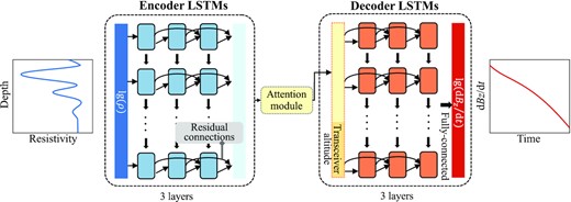
AEM simulator architecture. The LSTM network is composed of an encoder and a decoder connected by the attention module. Both the encoder and decoder have 3 LSTM layers here. Residual connection is introduced between layers. As the input information, normalized log-transformed resistivity values are fed into the input layer, while the transceiver altitude is incorporated into the weighted feature sequences. At the end of the LSTM network, the feature stream passes through a fully connected layer to output the predicted log-transformed AEM response.
Each layer in the encoder and decoder consists of 10 LSTM cells. Every resistivity model is cut into 10 segments and input into the LSTM encoder. The corresponding transceiver altitude scalar is repeated five times to form a vector of length 5, and then the vector is directly concatenated with every weighted vector transported from the attention module. The decoder is configured with a fully connected layer to finally output the predicted AEM signal, that is the logarithmic values of dBz/dt at all sampling points. The size of the LSTM cell state in the encoder is 40, while that in the decoder is 45 with the incorporation of transceiver altitude. The network configuration including its depth and width is further discussed in Section 3.5.
2.2 Data generation
A large sample set is necessary in ensuring the diversity and representation of the resistivity variations with depth to support the network training based on a full description of AEM induction laws, which directly affects the prediction performance of the data-driven AEM simulator. In this study, we generate 80 000 sample pairs for training set, each of which consists of a 1-D resistivity model with a transceiver altitude and the corresponding AEM response.
The resistivity model is generated first. Our study focuses on the underground medium down to a depth of 400 m, considering the commonly expected investigation depth of typical AEM surveys. We randomly determine the number (in the range of 1 and 15) of characteristic resistivities with a uniform distribution and their dominant depths above the bottom depth of the resistivity model, that is 400 m. Here we consider the application in most general inversion schemes where simpler models with fewer characteristic layers are preferred. For geological environments with more drastic resistivity variations, the model complexity in the training set must be increased accordingly. We randomly select the logarithmic values of characteristic resistivities from a normal distribution with a mean value of 2. Resistivities ρ are allowed to vary within the interval of 10−5–107 Ω∙m, which is sufficiently broad and thus ensures the adaptability of the simulator in practice. The discrete resistivity values are then interpolated by cubic splines onto a vertical grid with a uniform grid spacing of 2 m to obtain a continuously varying resistivity model. Thus, a smooth model with a total of 200 resistivity parameters is obtained. The resulting resistivity distributions at all depths for the training set are shown in Fig. 2(a), with the individual histograms at several different depths shown in Fig. 2(b) for examples. The resistivity distributions for all depths peak at ∼100 Ω∙m, while the percentages at the two ends of the resistivity range (10−5 and 107 Ω∙m) are much lower. The resistivity distributions at all depths are approximately normal. Hence, while the simulation accuracy for common media with moderate resistivity is enhanced, the LSTM network also acquires the ability to adapt to extreme resistivity values. The transceiver altitude ranges in 25–100 m according to common flight conditions and is uniformly distributed as shown in Fig. 2(c). We adopt the specifications of the AeroTEM IV system including the transmitting current and receiver configuration (Bedrosian et al. 2014). Given the resistivity model and observation mechanism, we calculate the corresponding time-domain AEM response dBz/dt by the forward modelling algorithm of Li et al. (2016), to serve as the target output of the AEM simulator. The time range of the AEM responses is 0.05–5 ms after the emission current is turned off, with 100 sampling points distributed uniformly on a logarithmic time axis. Consequently, the dimensions of the network input and output layers are 1 × 200 and 1 × 100, respectively. Since both the AEM response and the resistivity value span several orders of magnitudes, they are log-transformed to reduce their numerical ranges.
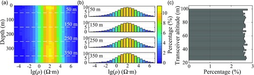
(a) Distributions of resistivity values at all depths in the training set (80 000 samples). White dash lines represent the depths at which the individual histograms are shown in (b). (b) Resistivity distributions at the depths indicated by the white dash lines in (a). (c) Distribution of transceiver altitudes in the training set.
Since AEM inversions usually adopt a roughness penalty to mitigate the ambiguity problem, here we consider that the underground resistivity variation with depth is characterized by layers with relatively smoothly varying properties. In addition, unlike the commonly used coarse grid in field applications considering the computational burden, we use a denser vertical grid to capture the fine changes of resistivity with depth and investigate the accuracy and efficiency of our approach to handling large number of model parameters.
2.3 Network implementation
3 RESULTS
3.1 Performance on the test set
Fig. 3 shows an example for a resistivity model arbitrarily selected from the test set. The accuracy of our AEM simulator is illustrated by the comparison between the prediction from the well-trained LSTM network with the target synthetic signal (i.e. AEM response of the same model selected from the test set calculated by the forward modelling algorithm of Li et al. 2016). The two AEM responses agree almost perfectly, with relative errors within ±1 per cent at all sampling points. This agreement indicates that the hidden mapping relationship between the resistivity models with transceiver altitudes and AEM responses has been successfully captured. We further examine the prediction performance for the entire test set. Fig. 4 shows the distributions of the relative errors at all sampling points. The mean values of the relative errors are close to zero, with an absolute maximum of 0.42 per cent. 75 per cent of the relative errors are concentrated within ±2 per cent, while 95 per cent of the relative errors fall in the range of ±5 per cent, indicating an overall prediction accuracy.
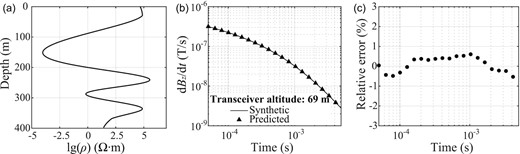
(a) An example of a resistivity model arbitrarily selected from the test set. (b) Comparison between the prediction by the well-trained LSTM network (triangles) and the target signal (solid line). (c) Relative errors (dots) between the two AEM signals in (b).
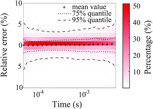
Distribution of relative errors between the LSTM-predicted and the target AEM signals for the entire 4000-sample test set at all sampling points. The red shading shows the percentage of the relative error within uniform bins of 1 per cent width at each sampling point. The plus signs represent the mean values of the relative errors. The dotted lines define the 75 per cent quantile of the relative errors, while the dash lines define the 95 per cent quantile.
3.2 Sensitivity to resistivity distribution
The resistivity values at all depths in the training set largely follow the normal distribution. We generate six half-space models with resistivity values distributed uniformly on the logarithmic axis (Fig. 5a) to investigate the effect of resistivity distribution on prediction accuracy. As shown in Fig. 5(b), all six LSTM-predicted signals show good agreement with the target AEM signals, and the corresponding relative errors in Fig. 5(c) illustrate the prediction accuracy in more detail. The relative errors for the half-space models with resistivity values of 10−2–106 Ω∙m concentrate around zero. In contrast, those for the highly conductive model with a resistivity value of 10−4 Ω∙m fall below −5 per cent. The drop in accuracy can be accounted for by the resistivity distributions in Fig. 2(b), where the percentage of resistivity values around 10−4 Ω∙m is quite small, which affects the representation ability. In fact, the resistivity range we consider is broad enough to cover most of the underground media in nature, with plenty of moderate values to strengthen the representation ability for common media. In particular, increasing the number of samples with extreme resistivity properties can effectively enhance the prediction accuracy in highly conductive/resistive conditions.
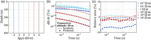
(a) Six half-space models with different resistivity values. (b) Comparison between the predictions by the well-trained LSTM network (triangles) and the target signals (solid lines) for models in (a). (c) Relative errors at all sampling points between the two sets of signals in (b) plotted by dots of the same colours.
3.3 Sensitivity to transceiver altitude
The changing altitude of the AEM transceiver directly affects the signal amplitude, which is taken into consideration in the range of 25–100 m in generating the training set. However, the actual transceiver altitude may exceed the range used in network training in certain areas such as around steep hillsides, in forests, and in volcanic areas. To examine the sensitivity of our network to the altitude variations, we generate a new test set using the same resistivity models in the original test set but with a transceiver altitude range of 20–140 m at a uniform interval of 20 m. Fig. 6 shows the prediction results for one arbitrary sample from the test set. The decaying trends of the AEM signals for all 7 transceiver altitudes (Fig. 6b) generated from the resistivity model (Fig. 6a) are quite similar, with the AEM signals recorded at lower altitudes showing higher amplitudes. The predictions by the LSTM network agree very well with the corresponding target signals at all altitudes. Fig. 6(c) shows the relative errors between the predictions and target signals at all sampling points. For the signals measured at altitudes from 40 to 100 m that are contained in the training set, the relative errors are very small, as we have seen in Fig. 6(c). For altitudes exceeding the preset range for the training set, the relative errors increase with the deviations of altitudes from the preset range. Nevertheless, all the relative errors for the test altitudes fall within ±5 per cent. For the entire set of 4000 resistivity models in the test set, the LSTM-enabled AEM simulator yields accurate predictions for all altitudes with average relative errors within the range of −2 to 4 per cent, as shown in Fig. 7.
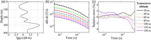
(a) An example of a resistivity model arbitrarily selected from the test set. (b) Comparison between the predictions by the LSTM network trained with the transceiver altitude range of 25–100 m (triangles) and the target AEM signals (lines) for 7 different altitudes ranging in 20–140 m at a uniform interval of 20 m. The dotted lines represent the results measured at altitudes within the preset range (25–100 m) in the training set, with the rest shown by the solid lines. (c) Relative errors at all sampling points between the two sets of signals in (b) plotted by lines of the same colour and style.
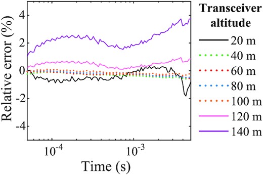
The average relative errors at all sampling points for the entire test set for the altitude range of 20–140 m at a uniform interval of 20 m.
Results from the new test set demonstrate the stable prediction performance of our AEM simulator for measurements acquired at altitudes within the preset range. The prediction errors grow slightly with the discrepancy between altitudes in the field and in training. To ensure prediction accuracy, therefore, we suggest using an appropriate range for the transceiver altitude in the training set with full consideration of practical operation circumstances.
3.4 Adaptability to discontinuously layered medium
The resistivity structures considered in the previous training set vary continuously with depth. However, there might be sharp interfaces underground with abrupt changes in electrical properties. We further examine the prediction performance of our AEM simulator for discontinuously layered media with abrupt resistivity changes, as shown by three examples in Fig. 8. We embed sharp interfaces at arbitrary depths in continuous resistivity models. For a model with a few interfaces (Model 1 in Fig. 8a), the AEM response predicted by the LSTM network is highly consistent with the target signal (Fig. 8b), with overall relative errors within ±1 per cent (Fig. 8c). The LSTM network performs equally well even for a model dominated by discontinuous resistivity variations (Model 2, Figs 8d–f). Even though the training pool consists entirely of models with smooth resistivity variations, the predicted AEM signal exhibits the accurate decaying trend of the electromagnetic field, demonstrating some degree of adaptability for unseen media with sharp resistivity interfaces. In general, deep learning community credits the strong performance of neural network algorithms to the ability of correctly interpolating the training data (Belkin 2021). Although the training set includes only smooth models, as the dominant depths and characteristic resistivity values are randomly generated, there are models with steep resistivity variations. Due to the volume effect of AEM method, it is sometimes difficult to distinguish between sharp and steep variations by their AEM responses. Thus, the adaptability to models 1 and 2 is mainly derived from the abundant resistivity variations in the training set. However, the adaptability is less stable since the sharp variation characteristics are not involved in the training set. For the model with a more complex interface distribution with depth, the relative errors for the LSTM-predicted signal exceed −20 per cent at later time (Model 3, Figs 8g–i), indicating a poor prediction performance. To improve the simulation accuracy of discontinuous resistivity variations, we conduct transfer learning (Pan & Yang 2009) based on the well-trained LSTM network by newly generated training samples considering the abrupt transition structures. We create 14 000 resistivity models following the generation strategy described in Section 2.2 and randomly embed no more than 5 stair-like resistivity layers into each model. A subset of 10 000 samples is used as the new training set, while another 4000 samples serve as the test set. The transfer learning converges at about 100th epoch with a time cost of 6 min. After transfer learning, the prediction errors of Model 3 by the newly trained network decrease significantly as shown in Fig. 9, indicating an improvement in simulation accuracy. Therefore, in cases where underground media are dominated by geological features under-represented in the training samples such as sharp interfaces, we suggest ensuring the sample diversity and adequacy and developing a more targeted network by transfer learning based on the well-trained network at a low cost, to further enhance the network adaptability. Meanwhile, it is also noteworthy that due to the inherent limitation of the data-driven method, the expanded adaptability is restricted to resistivity models with geological features that have been fully represented in the training samples.
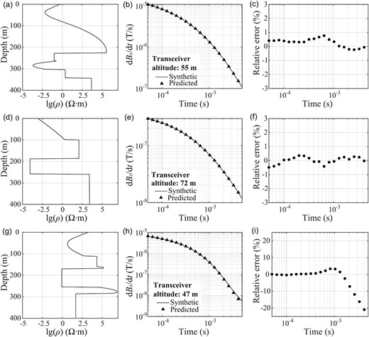
Prediction results for three synthetic resistivity models with abrupt changes. (a) Model 1 with a few abrupt changes. (b) Comparison of the network prediction (triangles) with the target AEM signal (solid line). (c) Relative errors (dots) between the two signals in (b). (d–f) Same as (a–c) but for Model 2, which is dominated by abrupt resistivity changes. (g–i) Same as (a–c) but for Model 3 with a more complex interface distribution with depth.
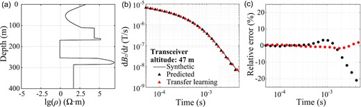
Transfer learning results. (a) Model 3. (b) Comparison between the prediction results of the original well-trained network (black) and the newly trained network by transfer learning (red). (c) Relative errors between the two sets of signals in (b) plotted by dots of the same colour.
3.5 Effect of network configuration on accuracy and efficiency
Our goal is to speed up the AEM signal prediction for a faster data inversion process. The network configuration involves two important hyperparameters: the depth and width of the network, which strongly affect the prediction efficiency of the AEM simulator. General speaking, for a given training set, deeper networks tend in practice to have greater representational ability than shallower ones (Rolnick & Tegmark 2018); and similarly, wider networks with a greater number of neurons per layer yield better natural accuracy (Wu et al. 2021c). However, the computational cost of the prediction stage increases with the size of the network, slowing down the subsequent inversion process. Here, we investigate the network performance by varying the number of layers in the network and the size of the LSTM cell states. Fig. 10 shows the average relative errors for all sampling points between the target AEM signals and predictions from different LSTM networks, as well as the corresponding time costs for the AEM signal predictions as functions of sample size. A shallow network, such as the 2-layer one, lacks the representation ability for complex non-linear characteristics and results in relatively low prediction accuracy (Fig. 10a). On the contrary, introducing more hidden layers improves the ability of feature extraction at the expense of efficiency. Similarly, a wider network with larger-sized LSTM cells can achieve more stable performance, but leads to greater prediction costs. Figs 10(b) and (d) show that the computational cost increases with the sample size at varying rates for all networks. For small sample sets (less than 1000), the growth of the time cost is relatively slow. When the size of the sample data set becomes larger than 1000, the time cost increases faster in proportion to the sample size. Our result suggests that a 6-layer network structure with an encoder-LSTM cell state of size 40 offers the best network performance. Nevertheless, there is no ‘one size fits all’ solution. The optimal network structure requires adaptation to practical data features and dimensions.

Accuracy and efficiency of different network architectures. (a) Average relative errors of the predicted results for the entire 4000-sample test set for all sampling points by the LSTM networks with different numbers of layers. The size of each cell state is fixed at 40 in the encoder, and 45 for the decoder with the incorporation of transceiver altitudes. (b) Prediction costs by the networks in (a) as functions of sample size plotted in the same colours. (c) Same as (a) but by the LSTM networks with different sizes of the LSTM cell states. Shown in the legend are the sizes of the cell states in the encoder, which are also the number of nodes in these cell states. In the case of the LSTM cell states of size 10 in the encoder, the size of cell states in the decoder is 12. In other cases, the sizes of the cell states in the decoders are 5 larger than those in the encoders. The number of layers is fixed at 6. (d) Same as (b) but by the networks in (c).
4 DISCUSSION
As a typical data-driven approach, our proposed AEM simulator extracts the mapping relationship between the resistivity models and corresponding AEM responses from the training set. To enhance the adaptability of the network, we enrich the sample diversity by choosing a broad range of resistivity values, generating random resistivity models, and expanding the size of the training set. The resistivity models we consider encapsulate most of the common geologic environments. The target AEM signals are simulated by the accurate forward modelling algorithm of Li et al. (2016), thus incorporating the electromagnetic induction laws into network training. Therefore, the physical properties of the AEM responses have been sufficiently described by the training samples. The data-driven AEM simulator is essentially guided by the physics of the AEM theory. On the other hand, due to the inherent limitation of data-driven deep learning methods, the prediction effectiveness depends largely on the data characteristics contained in the training set. For the occasional resistivity models dominated by extreme resistivity values or abrupt structural variations, the prediction accuracy may be relatively poor as the corresponding model characteristics are under-represented by less homologous samples. In these circumstances, transfer learning by new training samples with target characteristics can enhance the network performance at a low cost.
The well-trained LSTM network is restricted to being applied to the AEM simulation tasks for the same AEM system specifications and parametrization modes of resistivity models and AEM signals with the training set. In other words, it lacks the flexibility to be applicable to these different scenarios and thus network reconstruction is required, resulting in the inevitable time costs. Even so, we can still accomplish the training process in advance and accelerate the subsequent inversions. In our study, we adopt a relatively large number of model parameters as well as time sampling points than those of commonly used parametrization modes. Our synthetic analyses demonstrate that the LSTM-network simulator can deal with larger-dimensional input and output data, which facilitates more intensive time sampling and finer model parametrization in future AEM applications. When adopted to AEM data simulations for resistivity models discretized by fewer parameters or lower sampling rates, the LSTM network is required to be downscaled and retrained with newly generated training samples. Despite restriction of parametrization modes of resistivity model and AEM signal, a small-sized LSTM architecture can reduce the cost of calculation and further improve the forward modelling efficiency.
Our proposed AEM simulator achieves excellent accuracy with the relative errors mainly distributed within ±5 per cent at most sampling points. In practical scenarios, the AEM signal, whose amplitude is relatively low with a large decay rate, is usually contaminated by ambient noises. The typical data uncertainty in real cases is much larger than our prediction error (Andersen et al. 2016; Xue et al. 2020; Feng et al. 2021; Zhu et al. 2021; Sun et al. 2022). Several approximate forward modelling methods of AEM data have been developed and applied in field data inversion (Christensen et al. 2009; Auken et al. 2017). Christensen (2016) has demonstrated by field AEM data that using approximate forward modelling with a maximum relative error of 5.19 per cent, the inversion results are almost identical to those using accurate modelling. Therefore, considering the data uncertainty, the predicted AEM data with relative errors within ±5 per cent are acceptable in practical applications.
The AEM simulator can carry out signal predictions for ∼13 600 resistivity models within 1 s on a common PC (Fig. 8b). In contrast, it takes approximately 0.2 s for AEM data simulation of one model including parameter storage and signal calculation by the conventional modelling algorithm (Li et al. 2016), amounting to 5 models per second. The LSTM network can promote the forward modelling efficiency by ∼2700 times. For further comparison, the Fast Forward Modelling algorithm (Bording et al. 2021), which simulates the ground-based TEM data by a fully connected neural network, can calculate 208.3 forward responses per second on a single CPU for resistivity models with much fewer parameters, while the widely used conventional algorithms AarhusInv (Auken et al. 2015) and AirBeo (Kwan et al. 2015) deliver 16.2 and 11.8 TEM responses per second, respectively. Accordingly, our AEM simulator gains a significant advantage in computational efficiency among existing forward modelling algorithms.
Our eventual aim is to speed up the AEM inversion process with an accelerated forward simulation scheme, which has been achieved in several other geophysical methods. For example, Hansen & Cordua (2017) proposed a Markov chain Monte Carlo (McMC)-based sampling algorithm incorporated with neural-network-based forward modelling to invert ground penetrating radar data, which is demonstrated to be three orders of magnitude faster than conventional McMC inversion methods. Moghadas et al. (2020) obtained the 1-D inversion results of 6682 electromagnetic induction responses in half a day by the Bayesian algorithm with a neural network-based forward solver. Supported by the advantage in simulation efficiency, our proposed LSTM-network simulator has the potential to greatly accelerate the subsequent data inversion and uncertainty evaluation processes. Quantitative assessment of the AEM simulator in the improvement of inversion efficiency will be conducted in future studies.
5 CONCLUSIONS
In this study, we have developed a fast AEM simulator based on deep learning, which predicts directly the time-domain AEM response to underground 1-D resistivity structure with full consideration of the transceiver altitude. The AEM simulator is confined to generating the signals measured with the same AEM system characteristics as the training set. The predictions by the LSTM network agree well with the target signals, with the relative errors for the entire test set showing narrow distributions at all sampling points. The proposed approach achieves an overall promising accuracy for models with moderate resistivity values and yields adequate attention to the transceiver altitude. Carefully selecting an altitude range for the training samples to fully cover the practical situation is necessary to ensure the prediction performance. When the underground media contain resistivity anomalies with extreme values or drastic transitions, we suggest generating a new training set with the incorporation of the specific geological characteristics and using transfer learning to ensure the prediction accuracy at a low cost. The network configuration has a strong impact on the computational cost in the prediction stage. Our proposed approach is capable of predicting AEM responses rapidly for multiple resistivity models, reaching ∼13 600 model simulations within 1 s. With a much-enhanced efficiency, the fast 1-D AEM simulator has great potential to accelerate the subsequent inversion process. New opportunities lie in many inversion practices, such as introducing physical constraints into deep-learning algorithms and supporting the exhaustive sampling in non-linear inversion and uncertainty evaluation. AEM data inversion incorporated with the LSTM network-based AEM simulator will be investigated in future studies. In addition to facilitating AEM surveys, deep learning-based simulation workflow can be embedded into field data inversions for other geophysical applications under the layered-earth assumption, such as ground penetrating radar, tow transient electromagnetics, magnetotellurics, etc.
ACKNOWLEDGEMENTS
We thank the editor Rene-Edouard Plessix, Piyoosh Jaysaval and an anonymous reviewer for their constructive comments on the original manuscript. This research is funded by the National Natural Science Foundation of China (No. 42021003).
DATA AVAILABILITY
The data underlying this paper will be shared on reasonable request to the corresponding author.
