


SUMMARY
Microseismic monitoring is crucial for risk assessment in mining, fracturing and excavation. In practice, microseismic records are often contaminated by undesired noise, which is an obstacle to high-precision seismic locating and imaging. In this study, we develop a new denoising method to improve the signal-to-noise ratio (SNR) of seismic signals by combining wavelet coefficient thresholding and pixel connectivity thresholding. First, the pure background noise range in the seismic record is estimated using the ratio of variance (ROV) method. Then, the synchrosqueezed continuous wavelet transform (SS-CWT) is used to project the seismic records onto the time–frequency plane. After that, the wavelet coefficient threshold for each frequency is computed based on the empirical cumulative distribution function (ECDF) of the coefficients of the pure background noise. Next, hard thresholding is conducted to process the wavelet coefficients in the time–frequency domain. Finally, an image processing approach called pixel connectivity thresholding is introduced to further suppress isolated noise on the time–frequency plane. The wavelet coefficient threshold obtained by using pure background noise data is theoretically more accurate than that obtained by using the whole seismic record, because of the discrepancy in the power spectrum between seismic waves and background noise. After hard thresholding, the wavelet coefficients of residual noise exhibit isolated and lower pixel connectivity in the time–frequency plane, compared with those of seismic signals. Thus, pixel connectivity thresholding is utilized to deal with the residual noise and further improve the SNR of seismic records. The proposed new denoising method is tested by synthetic and real seismic data, and the results suggest its effectiveness and robustness when dealing with noisy data from different acquisition environments and sampling rates. The current study provides a useful tool for microseismic data processing.
1 INTRODUCTION
Microseismic events are very small earthquakes of generally negative moment magnitude generated during the mining, fracturing, and excavation processes (Mousavi & Langston 2016a; Chen 2018). Their locations can be used to estimate the fracture lengths and spacing. Microseismic monitoring has become an important tool for evaluating fracture treatments in excavation, fluid injection, or extraction (McGarr et al. 2002; Grigoli et al. 2017; Li et al. 2019; Palgunadi et al. 2019). The accuracy and precision of inverted locations in passive monitoring depend on the signal-to-noise ratio (SNR) of recorded microseismic data and the spatial distribution of the receivers. In practice, due to the relatively low amplitude of the microseismic wave, the observed seismic data is frequently contaminated by ambient noise. Therefore, seismic data denoising is a key issue in the microseismic study.
Several approaches have been proposed to improve the SNR by removing noise through signal processing processes while keeping key seismic signal properties. Spectral filtering is one of the most frequently used procedures. It attenuates some high- and/or low-frequency components where the noises are predominant. However, because the signal and noise frequently share the same frequency bands, spectral filtering is not always efficient. The portion of the signal may be filtered out with the noise, while the noise may not be totally removed. Furthermore, spectral filtering can produce artefacts prior to impulsive arrivals that might be misinterpreted as seismic signals (Scherbaum 2001; Mousavi & Langston 2017). Although spectral filtering may boost SNR, it does not guarantee that phase onsets or polarity would be simpler to detect (Douglas 1997). Effective seismic denoising methods can be achieved through more complicated techniques, such as principal component analysis (Hagen 1982; Huang et al. 2016c), empirical mode decomposition (EMD; Huang et al. 1998; Wu & Huang 2009; Han & van der Baan 2015; Chen et al. 2016a,b; Zhang et al. 2017), f–x or f–k filtering (Bekara & van der Baan 2009; Naghizadeh 2011; Naghizadeh & Sacchi 2012; Chen & Ma , 2014), singular value decomposition or singular spectrum analysis (Huang et al. 2016a, b), reduced-rank filtering (Velis et al. 2015; Bai et al. 2018) and least-squares complex decomposition method (Prony 1975; Chen 2018).
Time–frequency transform (TFT) is another effective and frequently used approach for microseismic data denoising. It aims to localize individual oscillatory components of the recorded signals. As seismic signals are non-stationary, time–frequency representation (TFR) can be used to track the time–frequency evolution of the spectral content of seismic data. It is more instructive to analyse their TFR rather than consider them in the frequency or time domain solely. Denoising in the time–frequency domain has the advantage over typical spectral filtering in that it allows one to separate the noise from the signal even if they are in the same frequency band. TFTs mainly include short-time Fourier transform (STFT) (Mousavi & Langston 2016a), continuous wavelet transform (CWT; Yoon & Vaidyanathan 2004; Mousavi & Langston 2016b; Zhao et al. 2020) and S transform (Parolai 2009; Wang et al. 2010, 2015). Recently, a new reassignment technique called synchrosqueezing (SS) was introduced as a powerful alternative to EMD (Daubechies et al. 2011). SS produces a sharpened TFR of the signal and highly localizes modulated oscillations. It might have better mathematical support and adaptability properties compared with EMD (Auger et al. 2013; Thakur et al. 2013; Herrera et al. 2014; Ahrabian et al. 2015). The synchrosqueezed continuous wavelet transform (SS-CWT) as a TFT method with higher resolution by incorporating CWT and SS, has been widely applied in signal processing and data analysis in different fields (Clausel et al. 2015; Liu et al. 2016; Mousavi et al. 2016c, 2017; Feng et al. 2017; Pan et al. 2020).
The wavelet-thresholding denoising method, which is adaptable and robust, determines which wavelet coefficients are essential based on the data's distribution feature (Donoho & Johnstone 1994; Donoho 1995). Because of its simple principle and outstanding denoising performance, the wavelet thresholding method has attracted extensive attention (Chang et al. 2000; Mousavi & Longston 2017; Langston & Mousavi 2019). The key research orientations are the construction of a thresholding denoising function and the selection of the wavelet coefficient threshold. Hard and soft thresholding based on universal threshold are the simplest but still popular thresholding denoising rules. On the other hand, Mousavi & Langston (2016a,b, c, 2017, 2019) proposed a variety of adaptive threshold selection methods for noise thresholding. However, because the background noise is not separated from the input data during the threshold estimation, it may result in an inaccurate estimate of the threshold and an unsatisfactory denoising effect. In addition, hard or soft thresholding rules only take advantage of the numerical difference between the wavelet coefficients of signal and noise. They might have difficulties when dealing with remaining noises of large wavelet coefficients.
In this paper, we provide a SS-CWT-based technique for automated noise removal for microseismic data, which incorporates determination of real-time pure background noise, wavelet coefficient thresholding, and pixel connectivity thresholding. The determination of the pure background noise range serves an accurate wavelet coefficient threshold, and the pixel connectivity threshold makes use of other useful information, namely the difference in image characteristics between signal and noise, to further improve the denoising effect. In the following sections, a brief theoretical introduction to the SS-CWT and wavelet denoising will be presented first. Then, details of the proposed method will be explained. At last, to investigate the robustness of the proposed approach for denoising, the algorithm will be evaluated by using synthetic data and field seismic data.
2 THEORETICAL BACKGROUND
If |$\tilde{\varphi }( \xi )$| is centrally distributed at |$\xi \ = {\omega }_0\ $|, the wavelet coefficients |${W}_s( {a,\tau } )$| will be scattered near the scale of |$a\ = \frac{{{\omega }_0}}{\omega }\ $|, resulting in a wide range of spectrum distribution with a fuzzy boundary and a low resolution in the time–frequency domain. To deal with this problem, the synchrosqueezed transform (SST) is used here to squeeze the energy into the real instantaneous frequency of the signal (Daubechies et al. 2011). The synchrosqueezed wavelet transform (SS-WT) rearranges the wavelet coefficients at the scale direction and makes the energy return to the real instantaneous frequency.
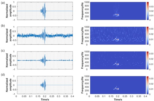
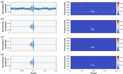
As an example, Fig. 1(d) shows sharpened TFR of SS-CWT compared with STFT (Fig. 1b) and CWT (Fig. 1c). The dominant frequency band of the signal can be identified from every TFR, whereas SS-CWT shows better time–frequency resolution performance.
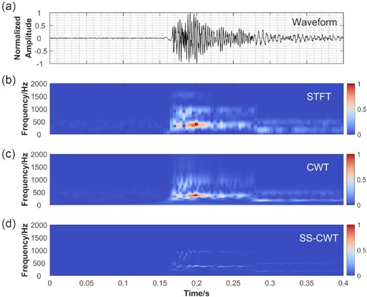
Time–frequency spectrum comparison of the same signal based on STFT, CWT and SS-CWT. (a) Field mine microseismic signal with high SNR, the sampling rate is 6000 Hz. Panels (b), (c) and (d) show the absolute values of STFT, CWT and SS-CWT of the time-series in (a), respectively, where CWT and SS-CWT are both based on the Morlet wavelet. Note that the absolute values of wavelet coefficients are normalized by the maxima in the corresponding time–frequency plane.
3 METHOD
3.1 Background noise estimation
Determining the wavelet coefficients threshold is a critical step in the denoising approach on the time–frequency plane. Donoho & Johnstone (1994) proposed an optimal threshold |$\lambda \ = \ \sigma \sqrt {2\log_{10}N} $|, also known as the universal threshold, for a signal with Gaussian noise of variance σ2, where σ is the noise level estimated from coefficients of the observed signal with N samples. In practice, the parameter σ is usually obtained from observed data including both seismic signals and background noise. It might encounter a biased estimation because of the discrepancy in statistical characteristics between signals and noise. Theoretically, the σ estimate performed by pure background noise is more feasible to quantify the noise level, which is beneficial to obtain a more accurate threshold. In this study, we proposed a simple technique to estimate the background noise range in the first step.
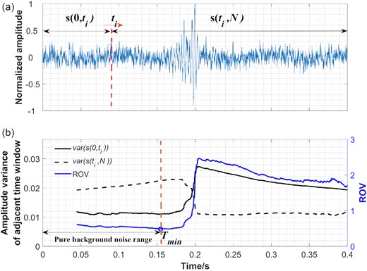
(a) Seismic data and schematic diagram of calculation of variance ratio. (b) Amplitude variances of two adjacent sliding time windows (black solid and dotted lines) and their ratio (blue line), where the blue circle is the minimum point of the ROV curve.
3.2 Hard thresholding based on empirical cumulative distribution function (ECDF)
3.3 Pixel connectivity thresholding in SS-CWT domain
After applying the hard thresholding of wavelet coefficients, a tiny amount of wavelet coefficients of noise remains in the time–frequency domain, which may obstruct the extraction of important information from the waveform. Several soft-thresholding forms have been developed to reduce residual noise interference (Weaver et al. 1991; Yoon & Vaidyanathan 2004; Liu & Xun 2014). In comparison to the wavelet coefficient of seismic signal, the wavelet coefficients of residual noise are highly dispersed and exhibit low pixel connectivity. Therefore, we proposed a new approach named pixel connectivity thresholding to remove the residual noise in this phase.
In image processing, if the edge of a pixel meets another in a 2-D image, the pixels are linked (Gonzalez & Woods 2007). The connected area can be calculated in two ways as shown in Fig. 3. Fig. 3(a) shows that if two adjacent pixels are connected in the horizontal and vertical direction, they are a part of the same connected component, and Fig. 3(b) shows that if the pixels are connected in the horizontal, vertical and diagonal direction, they are also a part of the same connected component. In this study, we chose the connected form of Fig. 3(b).
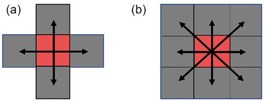
The pixel connected area in two different ways. (a) The pixels are connected in the horizontal and vertical directions. (b) The pixels are connected in the horizontal, vertical, and diagonal directions.
In the SS-CWT domain, pixel connection thresholding is a non-linear process that keeps wavelet coefficients if the area of the pixel linked components is bigger than Sthre; otherwise, they are set to zero and discarded. The residual noise component can be easily removed by pixel connectivity thresholding after scanning the object image and labelling the linked component. The SNR is further improved after pixel connectivity thresholding.
The whole process for denoising is as follows:
Estimate the pure background noise range using the ratio of variance (ROV).
Transform the observed waveform data into the time–frequency domain using SS-CWT.
Set the confidence value of P and obtain the corresponding wavelet coefficient threshold λ(a) at each scale a, based on ECDF of pure background noise determined in step (1).
Apply hard thresholding to process the data in the time–frequency domain.
Remove the residual noise by pixel connectivity thresholding.
Obtain the denoised signal by the inverse transform of SS-CWT.
4 RESULTS
4.1 Synthetic test
The denoising technique is applied to a known seismic signal that has been corrupted by synthetic noise. Fig. 4(a) shows a seismic signal with high SNR from field data recorded by a microseismic monitoring system in a metal mine. The sampling rate is 6000 Hz. The synthetic noisy data is generated by adding random noise, fixed frequency (20 and 100 Hz) noise and AM-FM noise to the seismic data in Fig. 4(a). As shown in Fig. 4(b), the SNR of synthetic data is reduced, and the onset of the seismic signal hardly be identified. The ROV curve of the synthetic data is shown in Fig. 4(c). It can be found that by searching the minimum of the ROV curve, the pure background noise range can be reliably determined. The background noise estimation method based on ROV is applicable to synthetic data and could provide an accurate, real-time dataset of background noise.
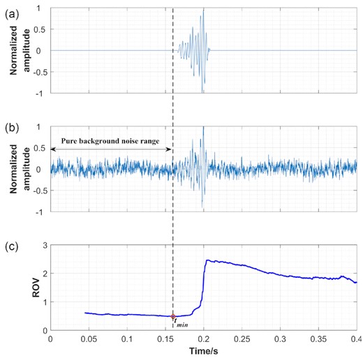
(a) The waveform of original synthetic data. (b) The waveform of synthetic noisy data. (c) ROV curve of synthetic noisy data, where the red hollow circle is the minimum position of the curve.
Fig. 5 shows the effects of each denoising step on the synthetic data. Fig. 5(a) demonstrates the original noise-free seismic signal and its TF representation with a prominent frequency of around 300 Hz. Fig. 5(b) shows the synthetic noisy data that is heavily contaminated by noise in every frequency band. The low SNR makes it difficult to determine the arrival time and polarity of the seismic signal. After most of the noisy wavelet coefficients are discarded by hard thresholding of wavelet coefficients based on the ECDF threshold, a distinct signal representation is obtained in Fig. 5(c). The pixel connectivity thresholding is then applied to the TF image (Fig. 5c) to clean up the highly dispersed noisy wavelet coefficients, providing a precise extraction of the signal energies in time–frequency domain, as shown in Fig. 5(d). After denoising, the SNR of the seismic data is greatly improved, and the onset of the seismic signal is clearly visible.
(a) The original seismic data and its SS-CWT spectrogram. (b) The synthetic data and its SS-CWT spectrogram. (c) The waveform and SS-CWT spectrogram of denoised data after hard thresholding based on the ECDF threshold. (d) The waveform and SS-CWT spectrogram of re-denoised data after pixel connectivity thresholding.
To see how the denoising process affects the polarity and the small emergent arrivals at the very beginning of the signal, which are buried behind the background noise, we examined the details of the denoised and original seismic signals in Fig. 6. It can be seen in Fig. 6(a) that the original and denoised seismic signals match quite well across the entire waveform with a high correlation coefficient of around 0.97. Furthermore, the onset time and polarity of seismic wave buried behind the noise become evident after denoising, and they are nearly identical to the original seismic signal, as shown in the zoomed time window in Fig. 6(a). The original seismic energies between 0.17 and 0.21 s have been recovered from the data without much modifying the time–frequency structure in the prominent frequency band around 300 Hz, which can give trustworthy seismic waveform information for further study (Fig. 6c). In the meanwhile, the background noise is precisely estimated (Figs 6b and d).
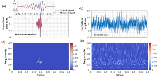
(a) Denoised waveform and its associated SS-CWT. (b) Extracted noise and its associated SS-CWT.
To demonstrate the superior performance of the suggested method, the output of our denoising strategy is then compared with those of frequency filtering and classic hard and soft thresholding (Donoho & Johnstone 1994; Donoho 1995) methods. Fig. 7 shows the original seismic signal, noise-contaminated signal and denoised signal using bandpass filtering (pass band is 150–450 Hz), hard-thresholding, soft-thresholding and the proposed approach, as well as their SS-CWT representations. The results show that most of the noise is removed while the energy of the valuable signals is well preserved. When picking the arrival information, those components preceding the first arrival are clearer and less distracting than the original noisy data. However, the band-pass filtering only removes noise with frequencies outside a certain band range, leaving noise in the prominent frequency band of the seismic signal unaffected. This results in a polluted waveform of first arrival (Fig. 7c). Both hard and soft thresholding keep the signal's structure (Figs 7d and e), but they are substantially less successful in removing noise than the proposed method in Fig. 7(f). A close examination of the initial arriving pulse in the zoomed window further demonstrates the superior performance of adaptive pixel connectivity threshold filtering over the other three.
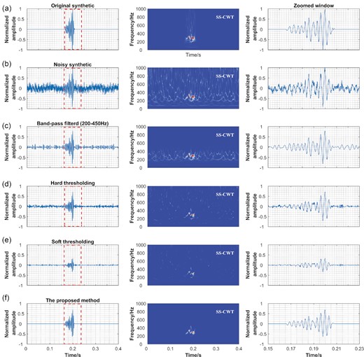
Comparison of different denoising methods and the proposed method. (a) The original seismic signal, its SS-CWT and magnified window of the seismic signal. (b) The synthetic signal, its SS-CWT and magnified window of the noisy signal. (c) The denoised signal, its SS-CWT and magnified window of denoised signal after bandpass filtering. (d) The denoised signal, its SS-CWT and magnified window of the denoised signal after hard thresholding based on the universal threshold estimated from the entire seismic record. (e) The denoised signal, its SS-CWT and magnified window of denoised signal after soft thresholding based on the universal threshold estimated from the entire seismic record. (f) The denoised signal, its SS-CWT and magnified window of the denoised signal using the proposed method.
Quantitative comparison analysis is further conducted, and the results of the RMSE (root-mean-square error), SNR and cross-correlation coefficient (CC) between the original seismic signal and denoised waveform using different approaches are shown in Table 1. The SNR is defined as the ratio of signal amplitude variance to the pre-event noise amplitude variance within a same window length. Compared with conventional methods, the proposed technique exhibits the lowest RMSE (0.0385), the highest SNR (>100) and CC (0.9694), suggesting its advantages in seismic signal denoising. It needs to be mentioned that the proposed method takes longer to calculate, but the time cost is still acceptable in practice.
Comparison of RMS, SNR, CC and time cost among different denoising methods.
| Method | SNR | RMSE | CC | Time (s) | TFT |
|---|---|---|---|---|---|
| Noisy data | 2.9018 | 0.1076 | 0.6277 | — | — |
| Band-pass filtering | 5.0711 | 0.0544 | 0.8540 | 0.03 | — |
| Hard thresholding | 7.5212 | 0.0545 | 0.8696 | 0.58 | SS-CWT |
| Soft thresholding | 9.5123 | 0.0767 | 0.8719 | 0.61 | SS-CWT |
| The proposed method | >100 | 0.0385 | 0.9694 | 0.78 | SS-CWT |
4.2 Field seismic data
First, we applied the denoising method to real microseismic data recorded during mining operations in a metal mine. The sampling rate is set to 6000 Hz to increase the locating accuracy. The high sampling rate makes microseismic event signal more susceptible to contamination of diverse environmental noise. Fig. 8 depicts the denoising effect of single microseismic event with different SNR. In all cases, using the proposed denoising approach achieved a significant increase in SNR. The denoising effect of microseismic signal waveform can be seen clearly in the denoised SS-CWT spectrum. The signal energies are almost fully retained. Furthermore, the onsets of seismic signal are plainly discernible from all denoised waveforms in the zoomed window. The denoising process enables one to obtain the first arrival time and polarity information easily with greater accuracy, which is crucial for source location and fracture imaging.
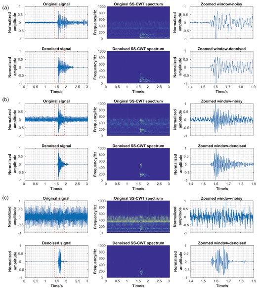
Denoised results for mining-induced microseismic records of (a) low, (b) moderate and (c) high SNR using the proposed method. The left-hand column is the original and denoised seismogram. The data in the red rectangle box is shown in the right-hand column using magnified windows. The middle column is the SS-CWT spectrum of the original and denoised signal. All waveforms are normalized by their maximum.
The denoising effect of a continuous multi-microseismic signal record in a metal mine is also tested, as shown in Fig. 9. It is impressive that a microseismic signal of tiny amplitude is retrieved after denoising, while being completely hidden in the background noise in the original waveform at about 1.4 s (black boxes in Figs 9e and f). The detection of minor microseismic events aids in the creation of a more comprehensive earthquake database, as well as crack imaging.
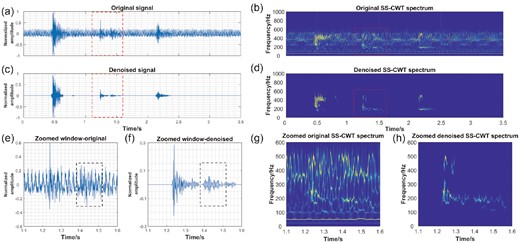
Denoised results for multi-microseismic record in a metal mine using the proposed method. (a) Original seismogram of several microseismic events induced by mining operation. (b) The SS-CWT spectrum of the original data. (c) Denoised seismogram and (d) denoised spectrogram. (e) Magnified windows of the original and (f) denoised signal in the red rectangle boxes shown in (a) and (c), respectively. (g) and (h) shows the SS-CWT representations of the seismic signal in (e) and (f), respectively. All waveforms are normalized by their maximum.
The second test set of real data is a monitoring example of hydraulic fracturing. 24 seismometers with sampling rate of 1000 Hz deployed at the surface were used to record microseismic events generated by water injection. Fig. 10(a) shows original microseismic data in one minute. In some channels the SNR is rather high, and the microseismic event signal is clear and distinct. While in other channels such as channels 1, 2, 9, 11, 18 and 19, the seismic signal is polluted by noise, resulting in a low SNR, and affecting the picking accuracy of the arrival time. Fig. 10(b) shows the denoised data using the proposed method. It can be found that microseismic signals of each channel are highlighted and plainly discernible after denoising. Fig. 11 shows the detailed results of the selected microseismic records from channels 18, 2, 11 and 1 in Fig. 11. The SNR of original microseismic record in these channels is graded from high to low, and some microseismic event signals are nearly drowned out by noise. From the original SS-CWT spectrum in Figs 11(b) and (d), we can see some high-energy components at the frequency about 50 Hz and its harmonics, which is probably associated with strong electronic noise. After denoising, the SS-CWT spectrum of microseismic events can be clearly observed, suggesting significant improvement in SNR for the selected four cases with different noise levels. These results demonstrate that the proposed denoising method is effective for microseismic monitoring data of hydraulic fracture. It should be mentioned that tiny noise remains after processing in Figs 11 (c) and (d), but it can be rule out based on channel consistency.
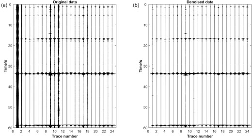
Denoised results of microseismic records during hydraulic fracturing based on the proposed method. (a) Original data. (b) Denoised data.
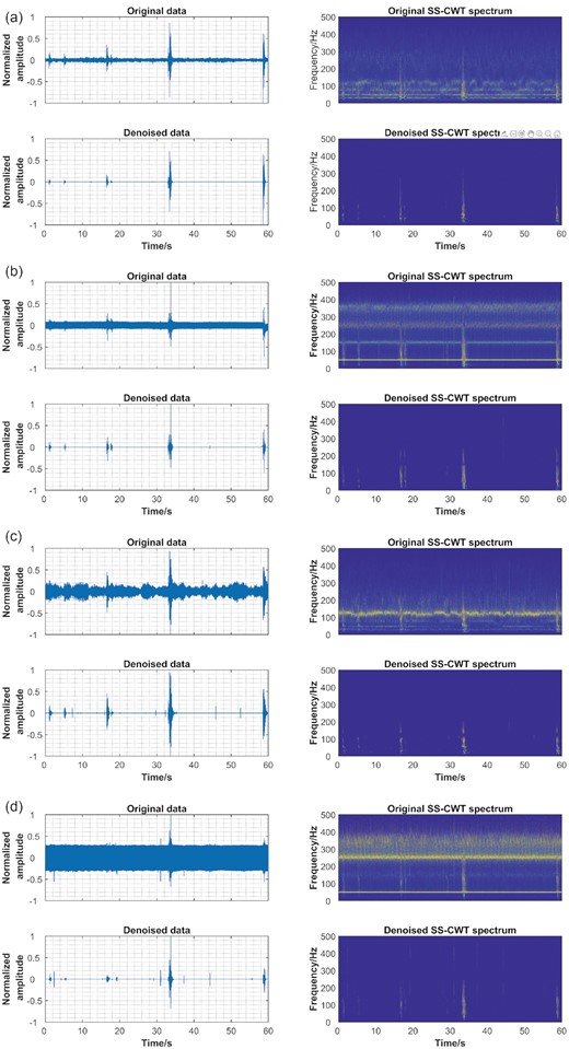
Denoised results of selected channels. (a) channel 18, (b) channel 2, (c) channel 11 and (d) channel 1. All waveforms are normalized by their maximum.
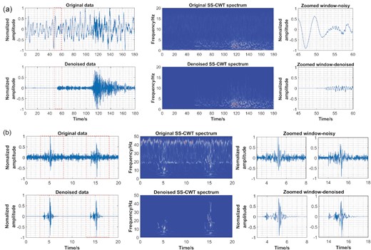
Denoised results of two natural earthquake signals. (a) The ML3.0 earthquake. (b) The ML0.5 induced microearthquake. All waveforms are normalized by their maximum.
The last test data are two natural earthquake records. One is the seismic signal of an ML3.0 earthquake observed at the ANMO station located at 34.95° latitude and −106.46° longitude. The epicentre distance is 3.72°. The data is obtained from the Incorporated Research Institutions for Seismology Data Management Center (IRIS DMC; www.iris.edu). The other is the signal of a ML0.5 microseismic event occurred during wastewater injection in Arkansas (Mousavi & Langston 2016a). The details of the test data are shown in Table 2. The P- and S-wave phases are obscured by the background noise, as shown in Fig. 12. Clearer P- and S-wave phases are visible after denoising. The denoising procedure could free up human attention to pick up seismic phases and provide more accurate P- and S-wave phase information that can help constrain the inversion of source parameters.
Detailed information of two test natural events.
| Date | Time (hh:mm:ss) | Latitude (°) | Longitude (°) | Magnitude | Depth (km) | Network | Station | Sampling rate (Hz) |
|---|---|---|---|---|---|---|---|---|
| 2022-08-15 | 23:39:34 UTC | 31.6465 | 104.4005 | ML3.0 | 6.98 | IU(IRIS/USGS) | ANMO | 40 |
| 2010-10-25 | 05:39:14 UTC | 35.29 | −92.3245 | ML0.5 | 4.4 | — | ARK1 | 100 |
For the first natural earthquake example in Fig. 12(a), the dominant low-frequency noise can be easily removed by bandpass filtering. However, bandpass filtering is ineffective for the noise that shares the same frequency band with seismic signal. While our proposed method can remove not only the dominant low-frequency noise, but also the noise in the same frequency band as the signal. Moreover, the dominant frequency band range of seismic signal recorded by the stations at different epicentre distances can be different. In practical, finding and setting proper pass-band range is another task and might be time consuming. Our proposed method enables one to obtain the feature of background noise timely and automatically. It is highly adaptive and can improve the working efficiency.
5 DISCUSSION
Wavelet coefficient threshold estimation is an important step in the process of denoising. It is worth noting that the purpose of the first step is to provide the range of pure background noise closest to the target seismic signal. This procedure enables that the statistical feature of background noise is obtained timely and accurately, which may bring advantage in determining the wavelet coefficient threshold. Fig. 13 shows the comparison of three thresholds for microseismic denoising in the synthetic test. The ER-universal and EN-universal thresholds are estimated from the entire record and the pure background noise using Donoho's method (Donoho & Johnstone 1994), respectively. The ECDF threshold (P = 0.99) is estimated from the pure background noise. In the frequency band 250–400 Hz, where the main energy of the seismic wave lies in, The ER-universal threshold is much larger than the ECDF and EN-universal thresholds, signifying an overestimation of the noise level. While in other frequency bands, where the statistical feature of background noise is not much affected by seismic wave, the ER-universal threshold is almost the same as EN-universal threshold.
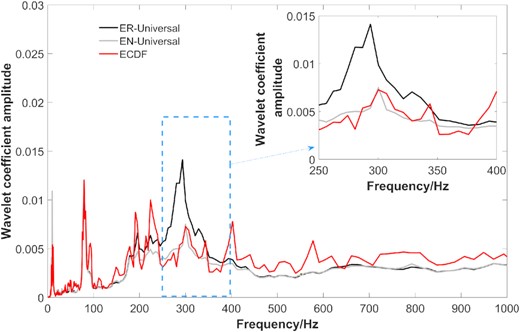
The comparison of three different thresholds, where ER-universal (black line) and EN-universal (grey line) thresholds using Donoho's method are obtained from the wavelet coefficients of the entire record and pure background noise, respectively, and the ECDF threshold (red line) is obtained from the pure background noise, where P = 0.99.
Langston & Mousavi (2019) revealed that the distribution of the absolute amplitude of the wavelet coefficients is not always Gaussian. Thus, using the ECDF approach may provide better estimates of the wavelet thresholds. In practice, the confidence value of the distribution (namely, P value) should be given to obtain the wavelet coefficient threshold of the pure background noise. It is necessary to explore the influence of P-value on the result of denoising. Fig. 14 shows the final denoising results of noisy synthetic data using different P values in the ECDF. It is found that the denoising effects are almost the same even though P value changes, implying that the proposed denoising method is not sensitive to parameter selection. Theoretically, using a smaller P value will lead to a lower wavelet threshold and cause more residual noise. However, these residual noises are mostly isolated and can be eliminated easily by pixel connectivity thresholding in the subsequent step, which ensures the robustness of the proposed denoising method.
Final denoised results using different ECDF confidence levels. (a) Synthetic noisy data, (b) P = 0.95, (c) P = 0.99 and (d) P = 0.995. All waveforms are normalized by their maximum.
The background noise range determined by the ROV method is critical for the subsequent denoising process. In practical, impulsive noise may affect the estimate of the range. To evaluate such influence, impulse noise is added to the synthetic data (Fig. 4b) at 0.05, 0.1, 0.13, 0.2 and 0.3 s, respectively, and all together. Then the new synthetic data with impulse noise are processed and the impacts on denoising results are explored. As shown in Fig. 15, the impulse does affect the estimation of background noise range (black triangle). However, the correlation coefficients between final denoising results and original seismic signal are all above 0.96, suggesting that the denoising results are still satisfactory. This is because that the determination of the wavelet coefficient threshold is based on the ECDF, which is independent of extreme values and not so sensitive to the number of samples in the background noise range. Moreover, the pixel connectivity thresholding plays a significant role in improving the final denoising effect. The integrated denoising process enhances the tolerance in the accuracy of the wavelet coefficient threshold and enables the application of the proposed method more flexible.
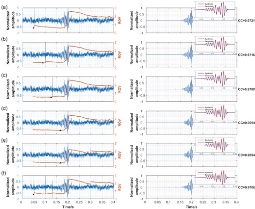
Final denoising results (after pixel connectivity thresholding) of synthetic seismic data with impulse noise at (a) 0.05 s, (b) 0.1 s, (c) 0.13 s, (d) 0.2 s, (e) 0.3 s, respectively and (f) all together. The background noise range is obtained from the minimum (black triangles) of the ROV curves. The CC represents the correlation coefficient between the denoising result and original signal.
It should be noted that when the estimated background noise range is short and not close to the target seismic signal, the fitting degree of first arrival and polarity would be affected, although the relatively higher CC reflects a good performance in amplitude preservation (Figs 15a, b and f). Considering the frequency of impulse noise is mostly higher than that of seismic signals, one possible solution is to apply a lowpass filter with high curt-off frequency before using the ROV method. Another way is that use the denoising result to redetermine the background noise range and then refine the wavelet coefficient threshold.
Concerning the anticipated future application, the proposed denoising method may be applicable to artificial intelligence which has been widely applied in variety of industry (Yu & Ma. 2021). Deep learning can be better used for denoising the time–frequency spectrum after transforming a 1-D waveform into a 2-D time–frequency domain (Zhu et al. 2019). However, training dataset with low SNR is generally hard to acquire. The proposed denoising approach can obtain clean and trustworthy denoising data, offering accurate sample labels for network training facing with field data with low SNR. It is worth mentioning that the proposed algorithm can also prepare the pure noise for ambient noise cross-correlation. In recent years, techniques for seismic imaging based on the empirical Green's function generated from the cross-correlation of background noise have been widely used (Shapiro et al. 2005; Bensen et al. 2007). Signal wavelet coefficients can be separated from the data without changing the time–frequency structure of the background noise in the surrounding areas using the proposed denoising method. It refers to the de-signalling process, which is crucial to the reliability of the surface wave extracted from ambient noise cross-correlation (Wapenaar 2004).
The proposed denoising approach presented satisfactory denoising results both in synthetic and field data tests. The method concentrates its strength on denoising single-channel seismic records. Although the multichannel manner may exhibit a more computational efficiency than the single channel, the expected satisfactory performance on most multichannel denoising methods relies on extensive geographic sampling. However, such demand for data acquisition is unattainable for most microseismic monitoring projects, especially for mine microseismic monitoring. It means the applied single-channel filtering can show better applicability to microseismic monitoring compared with multichannel one in poor conditions of data acquisition sites. Moreover, the proposed method can simultaneously process continuous multi-event and multiphase data, which could reduce the computational cost to a certain extent.
6 CONCLUSION
We proposed an adaptive denoising method combining wavelet coefficient thresholding and pixel connectivity thresholding based on the SS-CWT. In the denoising framework, the pure background noise range in the seismic record is estimated at first. Then, the wavelet coefficient threshold for each frequency is computed based on the ECDF of the coefficients of the pure background noise. After that, hard thresholding is conducted to process the wavelet coefficients in the time–frequency domain using the ECDF threshold. Finally, an image processing approach called pixel connectivity thresholding is applied to further remove isolated noise on the time–frequency plane. Performance of the proposed denoising method was tested using synthetic and real seismic data, and the results suggest its effectiveness and robustness when dealing with noisy data from different acquisition environments and sampling rates. The current study provides a useful tool for microseismic data processing.
ACKNOWLEDGEMENTS
This research is partly supported by Science and Technology Program of Shenzhen (grant no. JCYJ20210324104602006), Key Special Project for Introduced Talents Team of Southern Marine Science and Engineering Guangdong Laboratory (Guangzhou) (GML2019ZD0203) and Shenzhen Key Laboratory of Deep Offshore Oil and Gas Exploration Technology (grant no. ZDSYS20190902093007855).
DATA AVAILABILITY
The associated data and codes used by this paper are available at the link with https://github.com/sustechzzy/Denoising.
DECLARATION OF COMPETING INTERESTS
The authors acknowledge there are no conflicts of interest.
