


SUMMARY
The seasonal terrestrial water load modulation of seismicity is an important phenomenon to understand the mechanism behind earthquake triggering and nucleation. The presence of high-level seismicity and large seasonal water load amplitudes at the southeastern margin of the Tibetan Plateau provides a natural experimental environment for studying the modulation mechanism. The spatiotemporal distribution of the water load was inverted using Global Navigation Satellite System (GNSS) and Gravity Recovery and Climate Experiment (GRACE) data, and an earthquake catalogue (M ≥ 2.5) was declustered to obtain the background seismicity using the Epidemic Type Aftershock Sequences (ETAS) model. The Multichannel Singular-Spectrum Analysis (M-SSA) is adopted to the time-series of monthly averaged terrestrial water load and background seismicity rates, and the results show 1- and 2-yr periodicities in the seismicity rates and water load. The 1-yr periodicity in the seismicity rate is correlated with the rate of change of the monthly averaged water load. To evaluate the seasonal principal stress perturbations on the tectonic background stress orientations, the stress changes caused by the seasonal water load changes are projected onto the tectonic background stress field orientations constraining by 8 yr of earthquake focal mechanism solutions. The results show that the largest change of the seasonal principal stress perturbations is about 16 kPa. The number of excess earthquakes is evaluated with the background seismicity rates for discrete stress intervals. The results indicate a ∼10 per cent increase in the seismicity rates that correlate with the rates of the minimum and mean principal stress perturbations. The results above can be explained by the model of harmonic stress perturbations on rate-and-state fault. Based on this model, the nucleation period of the seasonal seismicity should be less than 1 yr at the southeastern margin of the Tibetan Plateau.
1 INTRODUCTION
Elastic stress accumulates by long-term tectonic forcing on a fault plane. After reaching or exceeding the critical value of the Earth's medium fracture stress, an earthquake will be triggered (Scholz 2019). Since tectonic activity is relatively stable, natural earthquakes generally have recurrence periodicities. However, the seismic activity is not stable over time. The main cause of the time delay or advance is the modulation of the stress perturbations caused by many factors, such as the dynamic triggering of earthquakes, solid earth and ocean tides, and seasonal mass load changes (Cochran et al. 2004; Gomberg & Johnson 2005; Métivier et al. 2009; Johnson et al. 2017a).
In studies of the influence of stress perturbations resulting from various physical processes on seismicity, the stress perturbations caused by seasonal mass load changes play a significant role. The magnitudes of the stress perturbations caused by seasonal mass load variations are large enough to affect seismicity (Johnson et al. 2017a, 2020). Meanwhile, the seasonal mass load variations have a relatively long stress loading period that can effectively trigger earthquakes (Dieterich & Linker 1992; Bettinelli et al. 2008). Researchers have reported that the stress perturbations caused by seasonal mass loads (e.g. terrestrial water, ice, snow, and the atmosphere) are significantly correlated with the seismicity of different regions around the world (Heki 2003; Craig et al. 2017; Johnson et al. 2017a,b, 2020; Xue et al. 2020; Dutilleul et al. 2021; Hsu et al. 2021; Perry & Bendick 2021). Of these, the surface deformation caused by the terrestrial water load variations is significantly greater than that due to the other seasonal mass loads in most areas (Fu et al. 2014; Johnson et al. 2017b; Hsu et al. 2020).
There are numerous large fault zones in the southeastern margin of the Tibetan Plateau, and the seismicity in this region is intense. At the same time, Global Navigation Satellite System (GNSS) observations show vertical seasonal crustal deformations with amplitudes greater than 20 mm in this region (Hao et al. 2016; Pan et al. 2018). All these factors mean that this region provides an ideal environment for studying the relationship between seasonal water load variability and seismicity. Previous studies in this region have found significant correlations between the equivalent water height from the time-series of the terrestrial gravity field provided by the Gravity Recovery and Climate Experiment (GRACE) and the seismicity in four subregions |$\sim 1^\circ \times 1^\circ $| where there are no M ≥ 4 earthquakes (Zhan et al. 2020). However, the seasonal seismicity in the entire study region is not investigated by now, and the mechanical relationship between seasonal water load and seismicity is still unclear for the whole study region.
In this study, we first combine GNSS and GRACE products to invert the spatiotemporal distributions of seasonal terrestrial water load at the southeastern margin of the Tibetan Plateau. The earthquakes are declustered using Epidemic Type Aftershock Sequence (ETAS) model to obtain the background seismicity. Then, the temporal correlation between water load and background seismicity rates is deduced by Multichannel Singular Spectral Analysis (M-SSA). In addition, we estimate the stress perturbations caused by these water load changes and project the stress tensors onto the orientation of the background tectonic stress derived from the focal mechanism solutions of earthquakes occurring in the region. Finally, we discuss the relationship between the stress perturbations and the background seismicity and investigate the seasonal terrestrial water load modulation of the seismicity at the southeastern margin of the Tibetan Plateau.
2 GNSS AND GRACE DATA
The GNSS data used in this work includes the results of 60 continuous stations (dots in Fig. 1) located at the southeastern margin of the Tibetan Plateau. They belong to the crustal movement observation network of China, with the data covering the period from July 2010 to July 2020. The data were processed using the Bernese 5.2 software (Dach et al. 2015) to obtain daily solutions based on the ITRF2014 reference frame. To invert the seasonal terrestrial water load of the study area (red square in Fig. 1), 45 virtual deformation stations (triangles in Fig. 1) were added to constrain the margin area of the study area (Fok & Liu 2019). Because the spatial interval of GNSS stations is about 2°, the spatial interval of virtual stations is also set to 2° to fill the position without GNSS stations. The vertical deformations of the virtual stations were deduced from the GRACE products representing the spherical harmonic expansions of the Mascon solutions provided by the Center for Space Research, the University of Texas (Save et al. 2016). Notice that the GRACE data used in this study denote the GRACE and GRACE-FO (Gravity Recovery and Climate Experiment Follow-on) data. The addition of virtual stations is to improve the inversion results of water load at the margin area of the study region, and this partition is discussed in the next section.
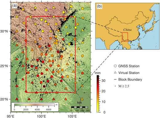
Spatial distribution of the GNSS and virtual stations. (a) Distribution of the stations. The dots and triangles denote the GNSS stations of the crustal movement observation network of China and the virtual stations whose movements were deduced from GRACE products, respectively. The colours denote the peak-to-peak vertical deformation of the stations. The red square denotes the study area. The black lines denote the boundaries of the blocks at the southeastern margin of the Tibetan Plateau (Zhang et al. 2005). The black points are M ≥ 2.5 earthquakes that occurred between 2010 and 2020. (b) The location of the study area with respect to the East Asian region.
We calculated the Love numbers using the surface load theory of Farrell (1972). Because the displacement of loading deformation is sensitive to the structure of a layered Earth above 150 km depth (Chanard et al. 2014), we replace the preliminary reference earth model (PREM; Dziewonski & Anderson 1981) with the averaged result of LITHO1.0 (Pasyanos et al. 2014) for the southeastern margin of the Tibetan Plateau and improve the accuracy of the Love numbers. The LITHO1.0 model is a 1° tessellated model of the crust and uppermost mantle of the earth, extending into the upper mantle to include the lithospheric lid and underlying asthenosphere. The spatial distribution of the peak vertical deformations is represented in Fig. 1, and the peak-to-peak values are about from 10 to 35 mm. Overall, the vertical deformations in the southern part of the study area are significantly larger than those in the northern area.
To study the relationship between the seasonal terrestrial water load and seismicity, the long-term tectonic deformation should be removed from the observed and deduced vertical displacements. Meanwhile, the offsets in the vertical displacement due to coseismic slip and instrument maintenance are corrected. We fitted a linear trend term and using these values determined a long-term trend which we removed from our time-series of the vertical displacements (Bevis et al. 2020). At the same time, the seasonal term is also fitted. Both the data of GNSS stations and the virtual stations were processed with the same method. As an example, the results for the GZSC GNSS station are shown in Fig. 2. The blue line and black curve in Fig. 2 are the long-term trend and seasonal term, respectively. The gaps in the GRACE and GNSS data sets are filled by using the Singular Spectrum Analysis (Yi & Sneeuw 2021). The temporal interval of the time-series is 1 month for GRACE and GNSS data.
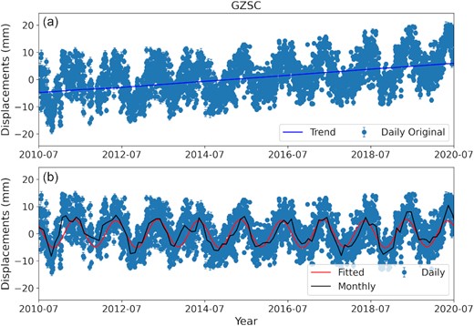
Vertical displacements of GZSC GNSS station from July 2010 to July 2020. (a) The blue dots with error bars denote the daily original data, and the blue line denotes the trend term calculated by fitting the displacement of 10 yr. (b) The blue dots with error bars denote the data after detrending, and the red line denotes the fitted seasonal term. The black line denotes the monthly averaged values deduced by the daily data.
We eliminate the effects of non-tidal ocean loading from the GNSS data using data from the international mass loading service (http://massloading.net/), and the seasonal amplitude of the non-tidal ocean load is less than 1 mm for the stations in Fig. 1. The vertical deformations recorded by the GNSS data are mainly caused by hydrological and atmospheric changes. However, the GRACE products do not include the effect of the atmospheric changes as they are corrected for this before release. Hence, to ensure the consistency of the GRACE and GNSS results for the terrestrial water load inversion, we follow the study of Fu et al. (2014) and remove the vertical deformations caused by changes in atmospheric load from the vertical GNSS deformations. The vertical deformation due to changes in atmospheric load changes is also from the international mass loading service, and the seasonal amplitude is 2–5 mm for the stations in Fig. 1. After the above processing, we obtained the deformation caused by the terrestrial water load variations, and the data are used to invert the spatial and temporal distribution of the terrestrial water load in the study region.
3 SEASONAL TERRESTRIAL WATER LOAD
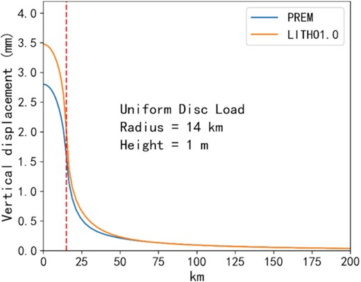
Disc-corrected Green's functions. The blue line denotes the Green's function deduced by the PREM model (Dziewonski & Anderson 1981). The orange line denotes the corrected Green's function deduced by the LITHO 1.0 model (Pasyanos et al. 2014). The red dashed line denotes the location of the radius of the disc. The radius is 14 km, and the thickness is 1 m.
The influence of the virtual stations was evaluated by using a checkboard strategy, with the results presented in Fig. 4. We note that the inverted results at the margin area which includes the virtual stations are better than when not using the virtual stations, which verifies the necessity of employing the GRACE products. Notice that the spatial resolution of vertical displacements of virtual stations should be the same as the GRACE products (∼350 km). Thus, the role of the virtual stations is not to increase the spatial resolution of the inverted results, but to improve the reliability of the inverted results at the margin area of the study region. In addition, owing to the spatial distribution of the GNSS stations, the resolution of the seasonal terrestrial water load is about 2° within the central area of the study region. The roughness factor β is obtained using the trade-off curve method, with the resulting value of β being 3 (Fig. 4).
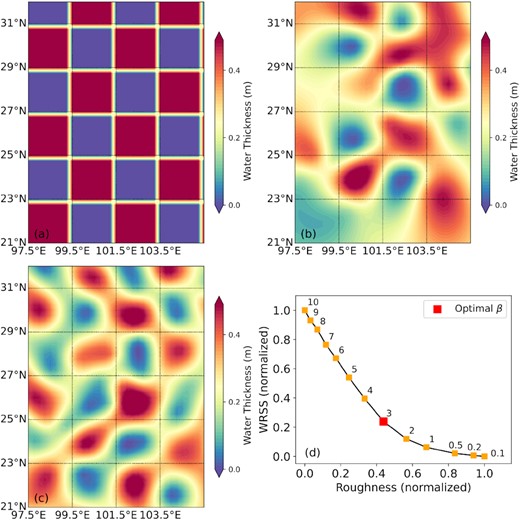
Inverse test at the southeastern margin of the Tibetan Plateau. (a) The distribution of the checkboard test. The water thickness is set to be 0.5 m. (b) Inverse results by using the GNSS stations in Fig. 1. (c) Inverse results by using the GNSS stations and virtual stations in Fig. 1. (d) Trade-off curve between the weighted residual sum of squares (WRSS) and roughness factors. Both WRSS and factors are normalized. The red square denotes the optimal result.
We obtain the spatial and temporal distribution of the seasonal terrestrial water load by repeating the inversion calculations on the vertical displacement for every month. The spatial distribution of the monthly averaged values of the seasonal terrestrial water load is shown in Figs 5(a)–(l). Meanwhile, the spatial amplitudes of the water load are extracted from the inverse results above, and the maximum amplitude is about 0.36 m (Fig. 5m). The seasonal terrestrial water load gradually increases from the northeast to the southwest of the study area. With the accumulation of summer precipitation, the water load amplitude in October with a maximum of ∼0.36 m (Fig. 5j). The periods of terrestrial water abundance and deficit are April to June and September to November, respectively. In addition, the spatial distribution of the seasonal terrestrial water load is consistent with the results deduced from GNSS data at Yunnan, southwest China (Jiang et al. 2021) verifying the correctness of the results above.
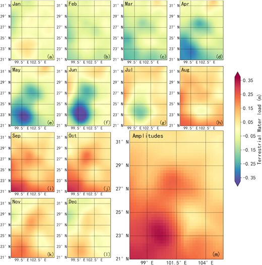
Spatial distribution of the monthly averaged values of seasonal terrestrial water load changes. The seasonal terrestrial water load changes are the inverse results from vertical displacements, the detailed information is in Section 3. The maximum amplitude of the water load changes is about 0.36 m.
The deformation detected by GNSS may include the deformation caused by hydrological loads outside the study region and the large wavelength loads at the global scale. Meanwhile, the potential sources of seasonal noise (e.g. draconitic noise) and systematic errors may interfere with the seasonal variations (Chanard et al. 2020). As a result, the terrestrial water height might be overestimated. However, the precise effects above are difficult to quantify due to the absence of GNSS data outside the study region and unmodelled or mis-modelled signals. In summary, the terrestrial water load inverted by the GNSS data is not completely accurate. However, the seasonal signals recorded by GNSS are mainly from the seasonal terrestrial water load. Although the terrestrial water load inverted by GNSS data has its limitations, this method can provide the results with a high spatiotemporal resolution based on the relatively dense distribution of GNSS stations. Thus, the influences of peripheral load are neglected in this study. With more data in hand and advances in models, these problems may be solved in a future study.
4 BACKGROUND SEISMICITY
The background seismicity has been correlated with seasonal mass loading at different regions around the world (Johnson et al. 2017a, 2020; Xue et al. 2020; Hsu et al. 2021; Perry & Bendick 2021). Because the aftershocks of a main shock in the study area are considered noise in the study of background seismicity, we remove the aftershock sequence from the earthquake catalogue using the ETAS method (Zhuang et al. 2002). Before earthquake declustering was conducted, we estimated the magnitude of completeness (Mc) using the entire-magnitude-range method (Woessner & Wiemer 2005). The result shows that the range of Mc is from 0.0 to 2.5 magnitude (Fig. 6). The earthquake catalogue considered in this work includes 672 585 events and is from the China Earthquake Network Center (data set S1) covering the period from July 2004 to July 2021, with the spatial range being extended by 3° from the edge of the study area (red square in Fig. 1) to ensure that the aftershocks of the larger earthquakes (e.g. 2008 Mw7.9 Wenchuan earthquake) can be included.
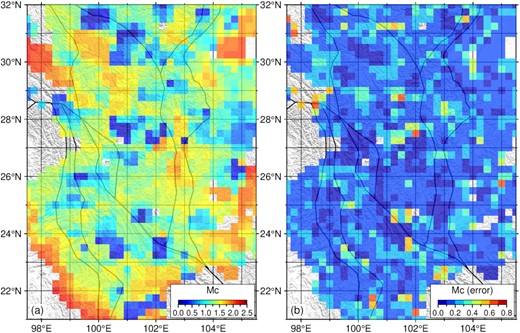
Spatial distribution of the magnitude of completeness (Mc) at the southeastern margin of the Tibetan Plateau. (a) Spatial distribution of the Mc deduced by the earthquake catalogue from China Earthquake Networks Center. (b) Spatial distribution of the corresponding Mc errors.
According to the results of the Mc analysis, the earthquake catalogue with magnitudes above 2.5 is declustered to obtain the background seismicity for the period between July 2004 and July 2020, covering the same time span as that considered for the seasonal terrestrial water loading analysis. Comparing the spatiotemporal distributions of the original and declustered seismicity (Fig. 7), the aftershocks are deemed removed from the original earthquake catalogue by the ETAS model. The total number of earthquakes during the study period (July 2010 to July 2020) with a magnitude ≥ 2.5 is 14 115, which after declustering was reduced to 3931.
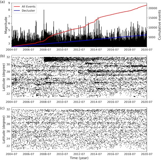
Original and declustered seismicity with the magnitude ≥ 2.5 at the southeastern margin of the Tibetan Plateau. (a) The cumulative seismicity, the black lines denote the magnitude of the earthquake and the shock time. The blue and red lines denote the original and declustered cumulative events, respectively. (b) The spatial and temporal distribution of the original seismicity. (c) The spatiotemporal distribution of the declustering seismicity. The ETAS model is implemented to decluster the earthquake catalogue.
We perform M-SSA (Craig et al. 2017; Golyandina & Zhigljavsky 2020) on the monthly declustered seismicity rate and averaged terrestrial water load changes (Figs 8a and e). The corresponding values of inverted terrestrial water load are extracted according to the epicentres of the background earthquake, then the extracted water loads for each month are averaged to form the time-series shown in Fig. 8(e). The M-SSA resulted in a trajectory matrix consisting of delayed copies of the different original time-series. Then, the covariance matrices between all pairs of time-series are computed using the trajectory matrix, and the singular value decomposition technique was then employed to obtain the eigenvectors for constructing the elementary matrices. Finally, the time-series components were calculated by diagonally averaging the elementary matrices. Because the covariance matrices are used to calculate each component of the original time-series, M-SSA extracts the shared information of each time-series. In addition, the weighted correlation matrix constructed by the time-series components is usually used to group the components that contain similar information (Golyandina & Zhigljavsky 2020).
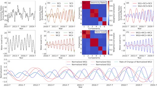
M-SSA of seismicity rates and time-series of seasonal terrestrial water load change. Panels (a) and (e) show the time-series of the seismicity rates and monthly averaged seasonal terrestrial water load, respectively. Panels (b) and (f) represent the first four components of the original two series above, and the SC and WC denote the seismicity component and water load components, respectively. Panels (c) and (g) show the weight correlation matrices of the first six components. Panels (d) and (h) are the results of the grouping and combining. SG and WG denote the seismicity group and water load group, respectively. Panel (i) shows the normalized results of (d) and (h). The solid and dashed lines denote the grouped results of the water load changes and seismicity rates, respectively. The cyan line denotes the rate of change of the normalized WG2.
The first four components of the seismicity rates and water load show approximately 1- and 2-yr periodicities (Figs 8b and f). At the same time, the weighted correlation matrices of the two series were calculated and used to group the above components. Because the weighted correlation values of the first and second components are close to 1 (Fig. 8c and g), the first two components that included the same information should be combined. Similarly, the third and fourth components should also be combined. The results show that the amplitudes of the 1-yr periodicity gradually increased over 10 yr, and the amplitudes of the 2-yr periodicity do not significantly change with time (Figs 8d and h). Meanwhile, the amplitude of the 2-yr periodicity of water load is weak.
To facilitate comparisons, the grouped results are normalized in Fig. 8(i). For the 1-yr periodicity, there is a relatively stable 3–4-month delay between the peak in seismicity rates (blue dash line) and the trough in water load (blue line). Compared to the 2-yr time, the delay or advance of the 2-yr periodicity between the seismicity rates (red dash line) and water load changes (red line) is not significant. Meanwhile, the rate of change of the water load (cyan line) is in phase with the 1-yr periodicity of the seismicity rate (blue dash line). The results above indicate, therefore, that the 1- and 2-yr periodicities of seismicity may be the result of seasonal terrestrial water load modulation, and the modulation mechanisms are explained in the discussion section.
In addition, the time-series of the seismicity rates and monthly averaged seasonal terrestrial water load (Figs 8a and e) are analysed using the stacked and spectral methods. On the one hand, the time-series are stacked in months for every 2 yr. The results show signals with approximate 1- and 2-yr periodicities. The 2-yr amplitude of seismicity rates is larger than the one of seasonal terrestrial water load (Fig. 9a) as a whole. A 3–4-month delay between the peak in seismicity rates and the trough in water load is similar to the results of M-SSA. On the other hand, the power spectral densities of the two series are calculated. There are 1- and 2-yr periodicities in both series at the same time (Fig. 9b). For the seismicity rates, the 2-yr periodic signal is more significant than the 1-yr periodic signal. For the seasonal terrestrial water loads, however, we find that the 1-yr periodic signal is larger than the 2-yr signal. The results of stacking and spectral analysis are consistent with the results of M-SSA.
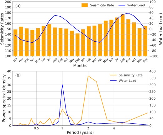
Results of the stacking and spectral analysis deducing from the time-series of seismicity rates and seasonal terrestrial water loads. (a) Stacked result in months for every 2 yr. The orange histogram and blue line denote the stacked seismicity rates and water loads, respectively. (b) Power spectral densities of the two series. The orange and blue lines denote respectively the power spectral densities of seismicity rates and water loads.
5 STRESS PERTURBATIONS
To compare the stress perturbation and seismicity, the perturbation stress tensors deduced by the seasonal terrestrial load changes should be projected onto the orientation of the background stress field (Johnson et al. 2017b, 2020). The principal orientations of the background stress field were inverted using the damped inversion method, which removes the stress rotation artefacts and resolves sharper stress rotations than smoothed method or a moving-window inversion (Hardebeck & Michael 2006). The focal mechanism solutions, including 534 solutions of earthquakes M ≥ 3.3 (data set S2) from 2009 to 2017 (Fig. 10), are from the China Seismic Experimental Site.
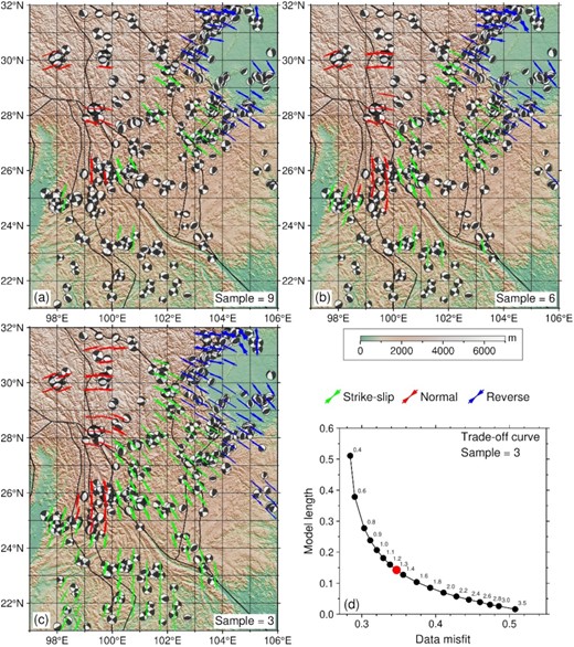
Background stress orientations at the southeastern margin of the Tibetan Plateau. (a) At least nine events in a grid patch, (b) at least six events in a grid patch, (c) at least three events in a grid patch, (d) the trade-off curve when at least three events are in a grid patch. The interval of the grids is 0.5°. The green, red and blue bars denote the strike-slip, normal, and reverse types of focal mechanism solutions, respectively. Beach balls in black and white are the focal mechanism solutions. Details can be found in data set S2.
After Johnson et al. (2020), we assessed the different minimum samples of the focal mechanism solutions to invert the orientation of the background stress and found that there are no significant differences between the results with different samples (Figs 10a-–c). The smooth factor was 1.3 in the case of the sample equalling 3 (Fig. 10d). The orientation of the maximum horizontal compressional stress shows a rotating pattern at the southeastern margin of the Tibetan Plateau, which is consistent with the horizontal velocities derived from the GNSS data (Wang & Shen 2020). The normal types of focal mechanism solutions are mainly distributed in the northwestern region of the study area, with the central and southern regions dominated by the strike-slip types and reverse types distributed over the northeastern region. The orientation of the maximum horizontal compressional stress is consistent with the previous studies in the Yunnan area (Wang et al. 2015; Tian et al. 2019), which verifies the procedures followed in this study.
The stress perturbations can be obtained by using Green's stress functions (Sun & Sjöberg 1999; She et al. 2021) and inverting seasonal terrestrial water load changes, with the Green's stress functions corrected using the same method as in Section 3. Considering the average depth of the earthquakes (M ≥ 2.5) around the southeastern margin of the Tibetan Plateau, we calculate the stress perturbations deduced by seasonal terrestrial water load changes at a depth of 10 km. Considering the spatial distribution of the background stress orientation, the calculated range of stress perturbations is the same as the patches in Fig. 10(c). Meanwhile, we projected the corresponding stress perturbation tensors to the background stress orientations. Note that the negative stress values denote compression, and the positive ones are tension. The annual peak-to-peak changes in the maximum principal stress |${\rm{\Delta }}{\sigma _1}$|, the minimum principal stress |${\rm{\Delta }}{\sigma _3}$|, the differential stress, |${\rm{\Delta }}({\sigma _1} - {\sigma _3})$|, and the mean stress |${\rm{\Delta }}({\sigma _1} + {\sigma _3})/2$| at a depth of 10 km are shown in Fig. 11. |${\rm{\Delta }}{\sigma _1}$| changes from 2 to 8 kPa, and |${\rm{\Delta }}{\sigma _3}$| changes from 4 to 16 kPa. The variation range for |${\rm{\Delta }}({\sigma _1} - {\sigma _3})$| is between 2 and 10 kPa, while the largest value of |${\rm{\Delta }}({\sigma _1} + {\sigma _3})/2$| is about 10 kPa.
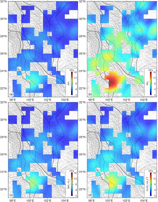
Annual peak-to-peak change of stress perturbations deduced by the seasonal terrestrial water load. (a) variations of the maximum principal stress |${\rm{\Delta }}{\sigma _1}$|, (b) variations of the minimum principal stress |${\rm{\Delta }}{\sigma _3}$|, (c) variations of the differential stress |$\Delta ({\sigma _1} - {\sigma _3})$| and (d) variations of the mean stress |${\rm{\Delta }}1/2({\sigma _1} + {\sigma _3})$|.
6 SEASONAL RESPONSE OF SEISMICITY
For the rates of the stress perturbations, delays of zero to six months in the seismicity rate were implemented, where the results show that the per cent excess seismicity |${N_{\mathrm{ex}}}$| has the strongest trend when the delay is zero (Figs 12a–d). The same test was implemented on the stress perturbations, and the results show that |${N_{\mathrm{ex}}}$| has the strongest trend when the delay is 4 months (Figs 12e–h). These results are consistent with the result of the M-SSA suggesting that the stress perturbations caused by water load control the seasonal seismicity.
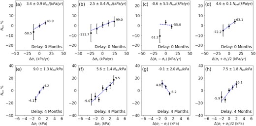
The per cent excess seismicity of the stress perturbations. Panels (a)–(d) are the per cent excess seismicity with no delay of stressing rates |${\rm{\Delta }}{\dot{\sigma }_1}$|, |${\rm{\Delta }}{\dot{\sigma }_3}$|, |${\rm{\Delta }}({\dot{\sigma }_1} - {\dot{\sigma }_3})$| and |${\rm{\Delta }}1/2({\dot{\sigma }_1} + {\dot{\sigma }_3})$|, respectively. Similarly, panels (e)–(h) are the results of stress perturbations with a 4-month delay. Negative and positive stresses denote compression and tension, respectively. The stress intervals are 1 and 12 kPa for the results of stress perturbations and their rates, respectively. The error bars denote the 95 per cent confidential intervals, and linear trends are fitted (blue dash lines). The values of the trends are represented with 2 standard deviations for each panel. The values at the end of the bins show the minimum and maximum range of the stress perturbations.
According to the criterion of Mohr's circle, the maximum principal stress |${\sigma _1}$| and the minimum principal stress |${\sigma _3}$| are the two sides of the circle. Meanwhile, the differential stress |${\sigma _1} - {\sigma _3}$| and the mean stress |$({\sigma _1} + {\sigma _3})/2$| are the radius and the centre of the circle, respectively. An increase in the radius or the movement of the centre in the tensional orientation will move the stress state closer to the critical plane, favouring the triggering of earthquakes. Our results show that the changing trends of per cent excess seismicity in |${\rm{\Delta }}{\dot{\sigma }_3}$|, |${\rm{\Delta }}({\dot{\sigma }_1} - {\dot{\sigma }_3})$| and |${\rm{\Delta }}({\dot{\sigma }_1} + {\dot{\sigma }_3})/2$| are consistent with the Mohr's circle encouraging the seismicity rates (Figs 12b–d). However, the trend of |${\rm{\Delta }}({\dot{\sigma }_1} - {\dot{\sigma }_3})$| is not as strong as the other two stress components. On the contrary, the changing trend of the per cent excess in |${\rm{\Delta }}{\dot{\sigma }_1}$| is opposite to the orientation of the triggering earthquakes (Fig. 12a). These results indicate an approximately 10 per cent increase in the background seismicity correlating with |${\rm{\Delta }}{\dot{\sigma }_3}$| and |${\rm{\Delta }}({\dot{\sigma }_1} + {\dot{\sigma }_3})/2$|. Similarly, the per cent excess seismicity of stress perturbations has the same change trend when the delay is four months (Figs 12e–h), while the results indicate an approximately 30 per cent increase in background seismicity correlating with |${\rm{\Delta }}{\sigma _3}$| and |${\rm{\Delta }}({\sigma _1} + {\sigma _3})/2$|. The strong trend of the minimum and mean principal stress indicates the reduction of the compression, encouraging seismicity. The results above are consistent with the results of M-SSA (Fig. 8i) and stacking (Fig. 9a), which confirms that the seasonal seismicity is correlated with the seasonal water load. Notice that the statistical analysis above actually includes seasonal and multiannual signals. However, considering that the seasonal variation of water load is significantly larger than the multiannual results (Fig. 9), the above analysis mainly responds to the results of seasonal signals.
7 DISCUSSION
The results of the M-SSA and the per cent excess seismicity indicate a complicated response of seismicity correlating with the seasonal terrestrial water load changes across the study area. The background seismicity rate and seasonal terrestrial water load both include 1- and 2-yr periodicities. There is a ∼ 30 per cent increase in background seismicity rates with a 4-month delay correlating with the stress perturbations caused by the seasonal water load. Meanwhile, there is a ∼10 per cent increase in background seismicity rates with no delay correlating with the rates of stress perturbations. According to the results above, the mechanism of seasonal water load modulation of seismicity is discussed below.
For 1-yr periodicity signal, on one hand, there is an approximately ∼30 per cent increase when considering a 4-month delay in the seismicity rates correlated with the stress perturbances |${\rm{\Delta }}{\sigma _3}$| and |${\rm{\Delta }}({\sigma _1} + {\sigma _3})/2$| (Figs 8 and 12). Based on the 1-D diffusion process (Shapiro 2015), if the depth is assumed as 10 km, a 4-month delay requires a hydrological diffusivity of approximately 0.8 m2 s−1, and this is not a reasonable value for the study region. The results indicate that increased mobility of pre-existing fluids inside the crust would change the pore pressure to modulate the seismicity rates via the seasonal water load changes (Johnson et al. 2020). On the other hand, there is an approximately ∼ 10 per cent increase with no delay in the seismicity rates correlated with the rates of the stress perturbances |${\rm{\Delta }}{\dot{\sigma} _3}$| and |${\rm{\Delta }}({\dot{\sigma} _1} + {\dot{\sigma} _3})/2$| (Figs 8 and 12). According to the models of harmonic stress perturbations on rate-and-state faults (Ader et al. 2014), when the stress perturbation periodicity is greater than the nucleation periodicity, the seismicity rate is in phase with the rate of the stress perturbation, e.g. events on dip-slip faults in California (Johnson et al. 2017a) and the Himalaya (Bettinelli et al. 2008; Ader et al. 2014). Based on the descriptions above, the results of this study are consistent with the rate-and-state model. Thus, the nucleation periodicity of the seasonal events should be less than 1 year in the study area.
As described above, both rate-and-state and pore pressure models can explain the mechanism behind the seasonal water load modulation of seismicity, and it is difficult to distinguish between them. When the delay time is long enough to obtain a reasonable diffusivity, the change of pore pressure can influence the seismicity directly (Perry & Bendick 2021). By contrast, if the delay time is too short when considering reasonable diffusivity values, the pore pressure caused by the mobility of pre-existing fluids inside the crust can also indirectly influence the seismicity (Johnson et al. 2020). It, therefore, seems that the pore pressure can always explain the delayed case of seasonal seismicity. However, the heterogeneity of faults and the differences in diffusivities in different regions, make the pore pressure mechanism implausible over the wider study area. The approximately 30 per cent of earthquakes induced by changes in pore pressure represent a high ratio, which requires a relatively uniform diffusivity across the study area. However, the distribution and types of faults are very complex, and the geological structure is also very different within the study area (Liu-Zeng et al. 2008). Thus, when the results suggest both rate-and-state and pore pressure mechanisms, the rate-and-state should be the more plausible option in the southeastern margin of the Tibetan Plateau.
According to the previous studies of seismicity and crustal strain rate (Kreemer et al. 2014), the seasonal seismic productivity and strain rates in the Himalaya (Ader & Avouac 2013), California (Johnson et al. 2017a), Tanganyika Rift (Xue et al. 2020), Northern Rocky Mountains (Perry & Bendick 2021) and this study area are shown in Table 1. The ranges of the strain rates in Table 1 are the 95 per cent confidence interval of the maximum shear rates and dilatation rates in different regions, and the averaged values are shown in brackets. The positive and negative values of dilatation rates denote the tension and compression, respectively. According to Table 1, seasonal productivities in different regions are not correlated with the magnitude of the strain rates. However, seasonal seismicity is relatively strong in regions dominated by compression (Himalayan Nepal) or tension (Tanganyika Rift). In other words, if the medium parameters are constant, the occurrence of seasonal seismicity may not depend on the magnitude of the background stress field, but on a uniform background stress field.
Strain rates and seismic productivity in different regions.
| Study region | Maximum shear rate (10–9 yr−1) | Dilatation rate (10–9 yr−1) | Seismic productivity (per cent) |
|---|---|---|---|
| Tanganyika Rift | 0–8.3 (3.3) | −3.3 to 15.0 (8.3) | ∼40 (Xue et al. 2020) |
| Himalayan Nepal | 0–65.8 (26.2) | −108.6 to 42.0 (-33.3) | ∼40 (Ader & Avouac 2013) |
| Rocky Mountains | 0–17.0 (4.2) | −25.6 to 21.1 (-2.3) | ∼20 (Perry & Bendick 2021) |
| California | 0–222.2 (54.5) | −141.3 to 128.6 (-6.4) | ∼15 (Johnson et al. 2017a) |
| This study | 0–51.5 (16.4) | −29.1 to 30.0 (0.4) | ∼10 (this study) |
The stress recovery after a great earthquake generally requires several years to decades (Parsons 2002; Tormann et al. 2015). When the crustal stress gradually increases and is close to the critical failure value, small stress perturbations would be more likely to trigger earthquakes. Thus, the increase in the amplitude of the 1-yr periodicity (Fig. 8d) may indicate an increase in crustal stress, which may reflect stress recovery following the 2008 Mw7.9 Wenchuan earthquake in the study area. In addition, according to the results from the previous studies (e.g. Heki 2003; Johnson et al 2017a, 2020) and our study, we infer the stress triggering threshold of the seasonal seismicity should be at least in the order of KPa.
The seismicity rates and seasonal terrestrial water load include a 2-yr periodicity, with this periodicity for the two-time-series being approximately in phase. It seems that the terrestrial water load caused the seismicity with a 2-yr periodicity. However, for the water load changes, the amplitude of the 2-yr periodicity is much smaller than that of the 1-yr periodicity (Fig. 8h). In contrast, for the seismicity rate, the amplitude of the 2-yr periodicity is greater than that of the 1-yr periodicity in the early part of the 10 yr (Fig. 8d). The stress perturbations caused by the water load changes may, therefore, be too weak to induce earthquakes. Thus, the 2-yr periodicity may be correlated with other factors and does not represent a seasonal influence, hence, requiring further research.
Finally, there are still some limitations in our analysis. On the one hand, the terrestrial water load and stress perturbations are determined by using a radially layered one-dimensional Earth model in this study. Due to neglect of the horizontal inhomogeneity of the Earth, the terrestrial water load and stress perturbation may be overestimated or underestimated. On the other hand, there are many earthquakes with large magnitudes in the study area, which may lead to inaccurate results of the declustering calculation. Therefore, despite the relatively reliable ETAS model is used here, the applicability of the model may also affect the results. In addition, the results of seasonal terrestrial water loads may be overestimated or underestimated due to the uneven spatial distribution of GNSS and the low resolution of the GRACE data.
8 CONCLUSION
In this study, the seasonal terrestrial water load modulation of seismicity in the southeastern margin of the Tibetan Plateau was investigated using both geodetic and seismic data. GNSS and GRACE data were used to invert the spatiotemporal distribution of seasonal terrestrial water load changes. The results show that the maximum amplitude of the water load change is about 0.36 m. The background seismicity is obtained by using the ETAS model. The stress perturbations induced by the water load variability at a depth of 10 km were then calculated and projected onto the orientation of the background stress deduced from focal mechanism solutions. Furthermore, the per cent excess seismicity of the stress perturbation is calculated to show the relationship between seasonal water load and background seismicity.
The results of the M-SSA between seasonal water load and background seismicity show that there are 1- and 2-yr periodicities in the time-series of the seismicity rates and seasonal terrestrial water load changes. Although the results of the M-SSA and the per cent excess seismicity associated with the stress perturbation changes suggest that the rate-and-state and pore pressure mechanisms can explain the seasonal terrestrial water load modulation of seismicity, considering the heterogeneity of the fault zones and the uncertainty of the area's hydraulic diffusivity, the rate-and-state mechanism is proposed to explain the seismicity induced by the water load changes. Thus, the results of per cent excess seismicity indicate an approximately 10 per cent increase in background seismicity, which is correlated with the rates of the minimum principal stress and mean stress perturbations. In addition, by comparing the strain rates and the seismic productivities in the different regions around the world where seasonal seismicity has been reported, we speculate that the occurrence of seasonal seismicity does not depend on the magnitude of the background stress field but a uniform background stress field.
ACKNOWLEDGEMENTS
This study is financially supported by the Special Fund of the Institute of Earthquake Forecasting, China Earthquake Administration (2020IEF0502), State Key Laboratory of Geodesy and Earth's Dynamics, Innovation Academy for Precision Measurement Science and Technology, Chinese Academy of Sciences (SKLGED2022-2-5), the Project funded by the China Postdoctoral Science Foundation (2020M680618) and the National Science Foundation of China (41874003). Thanks to Dr Weiwei Wu for providing the GNSS data.
DATA AVAILABILITY
GRACE data are available from http://www2.csr.utexas.edu/grace. The earthquake catalogue is from China Earthquake Network Center and supplied as data set S1. The focal mechanism solutions are from China Seismic Experimental Site and supplied as data set S2. Meanwhile, both data set S1 and data set S2 are uploaded in the open-access repository Zenodo (10.5281/zenodo.5 645 046).
