


SUMMARY
Here we qualitatively analyse the mass change patterns across Antarctica via independent component analysis (ICA), a statistics-based blind source separation method to extract signals from complex data sets, in an attempt to reduce uncertainties in the glacial isostatic adjustment (GIA) effects and improve understanding of Antarctic Ice Sheet (AIS) mass-balance. We extract the six leading independent components from gravimetric data acquired during the Gravity Recovery and Climate Experiment (GRACE) and GRACE Follow-On (GRACE-FO) missions. The results reveal that the observed continental-scale mass changes can be effectively separated into several spatial patterns that may be dominated by different physical processes. Although the hidden independent physical processes cannot be completely isolated, some significant signals, such as glacier melt, snow accumulation, periodic climatic signals, and GIA effects, can be determined without introducing any external information. We also observe that the time period of the analysed data set has a direct impact on the ICA results, as the impacts of extreme events, such as the anomalously large snowfall events in the late 2000s, may cause dramatic spatial and temporal changes in the ICA results. ICA provides a unique and informative approach to obtain a better understanding of both AIS-scale mass changes and specific regional-scale spatiotemporal signal variations.
1 INTRODUCTION
The Antarctic ice sheet (AIS) is the largest fresh water and thermal energy reservoir on Earth. It contains approximately 90 per cent of Earth’s land ice and approximately 70 per cent of Earth’s freshwater reserves. However, it is currently undergoing some of the most dramatic changes on Earth. These AIS changes are being driven by various external forcings, such as warming ocean waters (Alley et al. 2015) and global climate fluctuations, and can have significant implications on future global climate and sea level trends. Improved monitoring and assessment capabilities are therefore necessary to capture these AIS changes and advance our understanding of the drivers behind these ongoing changes.
The Gravity Recovery and Climate Experiment (GRACE) mission has been used to estimate regional- and ice-sheet-scale AIS mass changes since its launch in March 2002. Its successor, GRACE Follow-On (GRACE-FO), which was launched in May 2018, is currently used to continue monitoring AIS mass changes. Numerous studies have indicated accelerated AIS mass loss using GRACE/GRACE-FO data (e.g. Shepherd et al. 2012; King et al. 2012; Velicogna & Wahr 2013; The IMBIE team 2018). However, the GRACE/GRACE-FO measurements consist of the superposition of gravity changes due to different physical processes along the radius, including atmosphere, ocean, terrestrial water storage, and solid Earth changes. In particular, the redistribution of the near-surface solid Earth due to glacial isostatic adjustment (GIA), which is the ongoing response of the solid Earth due to changes in the ice–ocean load following the Last Glacial Maximum, has a direct impact on the inferred AIS mass changes from satellite gravity measurements (Wahr et al. 2000).
However, sparse in situ observation networks across Antarctica have led to the inability to effectively constrain the GIA effect, with this effect possessing the dominant uncertainty in AIS mass balance estimations. Numerous approaches have been proposed to constrain the GIA effect, such as joint analyses of GRACE/GRACE-FO data and either global positioning system (GPS, Wang et al. 2013; Hattori et al. 2021) or Satellite laser altimeter, Ice, Cloud, and land Elevation Satellite (ICESat) data (Wahr et al. 2000; Riva et al. 2009). Statistical methods, such as principal component analysis (PCA), have also been introduced to analyse GRACE-derived signals (Schmidt et al. 2008; Schmeer et al. 2012; Talpe et al. 2017). Independent component analysis (ICA) is another effective method for understanding complex processes that has been proven to possess the potential to separate spatiotemporal GRACE-derived mass changes into independent components (Forootan & Kusche 2012).
One disadvantage of PCA is that PCA extracts the primary components according to the variance distribution of a measured geophysical field, which always leads to the extraction of the stronger signals and the potential dismissal of relatively weak but highly independent signals. PCA-extracted features are statistically uncorrelated to each other, which means that signal mixing remains a problem (Cardoso 1992). ICA takes a different approach to PCA in exploring a data set by treating all of the components equally. The goal of ICA is to find a linear transformation that can decompose the observations into independent components using high-order statistics.
Forootan & Kusche (2012) were the first to use ICA for GRACE data analysis. They conducted both PCA and ICA to analyse the simulated synthetic data, compared the results with real GRACE products, and found that the ICA results were closer to ‘optimal decomposition’, which indicated that ICA may be more suitable approach for solving the problem of unknown source signal decomposition. Awange et al. (2014) successfully separated the independent water storage patterns in the Nile sub-basins using ICA, and related them to climate indices (e.g. El Niño-Southern Oscillation and Indian Ocean Dipole).
Banerjee & Kumar (2018) used ICA to analyse the variations in various components of an Indian hydrological system. Anyah et al. (2018) used it to derived the relationship between land water storage changes in Africa and global climate indices. Shafiei Joud et al. (2019) determined the ICA-derived GIA uplift in Fennoscandia and Laurentia using GRACE data, and obtained comparable results to regional GPS observations.
ICA may therefore be an appropriate approach for solving the uncertainty in the source signal and constraining the mixing pattern in Antarctica. Here we use ICA to extract the spatial and temporal patterns of AIS mass changes from GRACE and GRACE-FO data. We expect ICA to potentially provide a new perspective for elucidating the physical processes driving AIS mass changes.
2 DATA AND STUDY AREA
2.1 GRACE and GRACE-FO data
The GRACE and GRACE-FO Level-2 products are mainly provided by the three official data centres: the Jet Propulsion Laboratory (JPL), the Center for Space Research (CSR), and the German Research Centre for Geosciences (GFZ). We used the Release 06 spherical harmonic (SH) coefficient published by the three official data centres, which included all of the available GRACE/GRACE-FO data during the April 2002–June 2020 period, with a data gap from July 2017 to June 2018. We found considerable discrepancies among the data sets provided by the different data centres (Appendix A), which could be due to the processing applied by each data centre. We simply took the average of the SH coefficients from the three data sets as our input data to avoid any bias in an individual data set.
We applied standard post-processing methods to all of the SH coefficients. These included C20 replacement for all of the GRACE and GRACE-FO solutions and C30 replacement for the GRACE-FO solutions using coefficients derived from satellite laser ranging provided by the Goddard Space Flight Center (Loomis et al. 2020), SH coefficient truncation up to 60 order and degree to suppress high-frequency noise, and the use of a DDK4 filter for smoothing (Kusche et al. 2009). Although there is an approximately 1-yr gap between the two missions, Velicogna et al. (2020) have demonstrated that the GRACE and GRACE-FO time-series can line up well across the data gap in Antarctica. Furthermore, the final year of data acquired at the end of the GRACE mission (July 2016–July 2017) was not used due to deteriorating GRACE observations. However, data continuity is not an issue in ICA analysis, such that there is no need to fill this 2-yr gap (July 2016–May 2018) and other lacked months in the time-series. Notably, as an important original signal, GIA was not given special treatment by any model in this study.
2.2 Overview of the Antarctica mass changes
The mass input and output processes across the AIS system can assist in interpreting the observed GRACE/GRACE-FO mass changes. Surface mass balance (SMB) analysis can be used to estimate the snow and ice variations across the AIS surface, with a particular focus on snowfall, rainfall, surface sublimation, and drifting snow sublimation (Van Den Broeke et al. 2004). However, some regionally important processes, such as drifting snow sublimation, might have a negligible impact on the SMB at the GRACE/GRACE-FO resolution (AIS scale, van Wessem et al. 2018).
The mass input is driven mainly by snowfall (Boening et al. 2012). There are great regional differences in the AIS SMB, with a significant coast–inland decrease in the precipitation gradient owing to the moisture air masses decreases as they migrate onto the Antarctic Plateau. The mass output is attributed mainly to ice discharge through melting of glaciers. There are seasonal variations at the annual scale that are driven by meteorological factors, such as the strongest melting occurring during the austral summer (Liston et al. 1999). Glacier melting may be ocean-driven at medium- to long-term scales (Pritchard et al. 2012; Hirano et al. 2020), whereas it may be determined by topography and ice shelf stability at the long-term scale. GIA is also an important solid-Earth signal that could be derived from satellite gravimetry.
Therefore, there are a number of components that may be statistically independent integrated in GRACE/GRACE-FO observations, such that they can be separated via ICA. These include: (1) atmospherically related high-frequency (seasonal) signals, such as snow and seasonal melting; (2) medium- to long-term (several years) increases/decreases in ocean-driven cycles of precipitation and glacier melting; (3) long-term glacial melting owing to topography and (4) solid-Earth-induced GIA.
We derived the mass change trend in Antarctica using a simple linear regression model (linear term only), as shown in Fig. 1, with the mass changes over the analysed time-series expressed in equivalent water height (E.W.H). It can be seen that the mass changes are primarily concentrated in the following areas: (1) Significant mass loss in the Amundsen Sea Sector (AMS), West Antarctica, and Bellingshausen Sea Sector, Antarctic Peninsula; (2) significant mass gain across Dronning Maud Land (DML) and Enderby Land (EL), East Antarctica; (3) mass loss across Totten Glacier in Wilkes Land (WL) and Ninnis Glacier in George V Land (GVL), East Antarctica and (4) mass gain across the Ross Ice Shelf (RIS), Filchner-Ronne Ice Shelf (FRIS) and a portion of Marie Byrd Land (MBL), West Antarctica. Previous studies have indicated that these mass changes are due to the superposition of the following processes: (1) The large mass loss in the AMS is primarily due to the accelerated melting of glaciers in the Amundsen Sea Embayment, especially Pine Island Glacier (Mouginot et al. 2014; Harig & Simons 2015). (2) The mass gain in DML and EL is primarily due to anomalous snowfall events in 2009 and 2011 (Boening et al. 2012). (3) The mass loss in the Totten and Ninnis regions (WL and GVL, respectively) are primarily due to the melting of local glaciers, including Totten, Ninnis, and Mertz glaciers (Rignot et al. 2013; Li et al. 2016). (4) The RIS shows a positive trend without any GIA correction, whereas a negative trend is observed after including the GIA effect, which suggests that the GIA effect has a significant impact on this region.
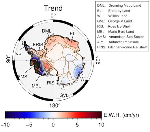
Regression trend of AIS mass change via a linear model of the April 2002–June 2020 GRACE/GRACE-FO data. Brown dashed lines represent the drainage basin boundaries across the AIS, which are derived from historical observations, a modern-day digital elevation model, and ice-velocity data from Rignot & Mouginot (2012).
We can find that the AIS mass change trends are primarily dominated by strong glacier and snow signals, and that the influences of glacier melt and snow accumulation are particularly significant compared with other signals. Here we attempt to recover these identifiable source signals from the overall mass change trend, isolate the factors that affect AIS mass balance, and advance our understanding of the spatiotemporal characteristics of observed AIS variations.
3 METHOD
ICA is an analytical method that decomposes complex mixing of source signals into statistically independent components (ICs) via the use of higher-order statistics (usually fourth-order moment (kurtosis) or entropy). ICA can utilize the statistical characteristics of GRACE data to explore potential signals without any prior information. ICA should be a viable approach for analysing GRACE-like observations since they generally consist of non-Gaussian data distributions, particularly since the high-order statistics of these data will not be considered by PCA (Forootan & Kusche 2012).
Bell & Sejnowski (1995) demonstrated that ICA can contrive the ICs of a data set, even if the underlying sources are not statistically independent. Therefore, ICA may find the independent signals that are not the underlying sources. GRACE observations build on a data matrix, X, with n grids and p epochs.
sICA can find a series of spatially independent components and their corresponding time-series. sICA assumes that |$\widetilde{U}$| can be decomposed as |$\widetilde{U}=SA_S$|, AS is a k × k mixing matrix, and S is a statistical independent matrix of the spatial vectors. The scaled original signal, |$y_{s_i}=\widetilde{U}W_S$|, can therefore be recovered by the unmixing matrix, WS, where |$W_S=A_S^{-\mathbf {1}}$|.
tICA can find a series of temporally independent components and their corresponding spatial vectors. tICA assumes that |$\widetilde{V}=TA_T$|, AT is a k × k mixing matrix, and T is a statistical independent matrix of the time-series. The scaled original signal, |$y_{s_i}=\widetilde{U}W_T$|, can therefore be recovered by the unmixing matrix, WT, where |$W_T=A_T^{-1}$|.
4 RESULTS AND DISCUSSION
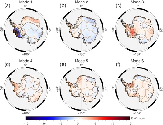
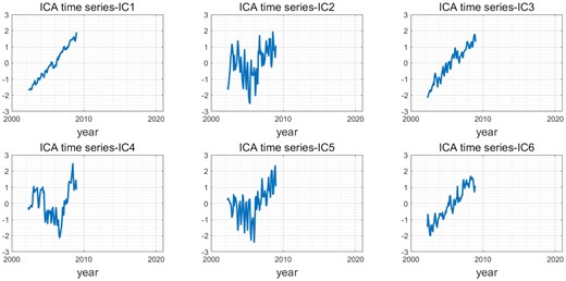
PCA is used as a pretreatment for centring and dimension reduction. The first six principal components, which describe more than 70 per cent of total variance, are used as the ICA inputs in this study. sICA will produce spatially independent modes over the study region, and their corresponding time-series should exhibit the temporal characteristics of separate subregions. Fig. 2 shows the results of the first six ICA-extracted spatial modes, with their corresponding time-series (IC1, IC2, IC3, ..., IC6) given in Fig. 3. All of the temporal modes are been normalized in this study.
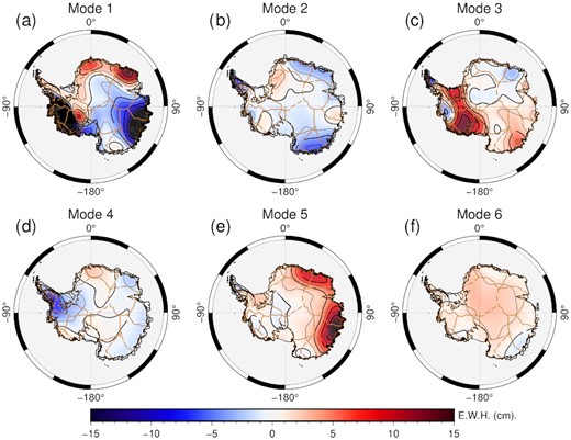
The first six ICA-extracted spatial modes for the entire study period.
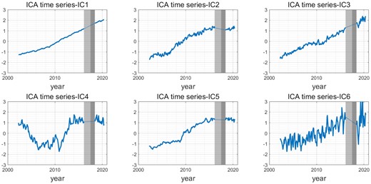
Corresponding time-series of the decomposed spatial modes in Fig. 2. The grey shading denotes the data gap in the study period, with the GRACE/GRACE-FO gap (July 2017–May 2018) in dark grey and the discarded period (July 2016–July 2017) in light grey.
4.1 Long-term trend
There are three long-term components, Mode-1, Mode-2 and Mode-3, among the six ICs. Mode-1 spatial pattern (Fig. 2a) is very similar to the regression trend (Fig. 1), and its corresponding time-series (IC1) shows a clear linear trend. Mode-1 mass changes are primarily distributed across the well-known glacier regions, as mentioned in Section 2.2, such as the large mass loss in the AMS and Bellingshausen Sea Sector, West Antarctica, mass loss in WL and mass gain across DML and EL, East Antarctica.
However, some subtle differences may suggest potentially different meanings of the Mode-1 signal. We find that the mass loss signal in the WL region is significantly spatially wider than the regression signal, which may be an indicator of basal melting along the Totten glaciers in this region. A comparison with the Bedmap2 bed topography (Fretwell et al. 2013) revealed that the mass-reducing area coincided with the deepest bed topography in this region. Hirano et al. (2021) indicated that the potential basal melting along Totten Glacier was caused by relatively warm Circumpolar Deep Water transport. Despite the risk of instability due to the regional bed topography, this sector remains in a stable state (Morlighem et al. 2020). Therefore, it may reveal a possible connection between the observed mass loss and the bed topography. Furthermore, the northern tip of the AP, which is dominated by strong seasonal changes, is not included in the Mode-1 signal. The RIS also shows a negative trend where the AIS mass loss is overwhelmed by GIA and a positive trend in the regression trend with no GIA correction. The above details suggest that the Mode-1 signal can be largely attributed to glacier changes.
The Mode-2 captures information on the glaciers that are not captured by the Mode-1. This signal, in combination with its corresponding time-series, IC2, indicates that these regions are in a relatively balanced state between 2002 and 2006, and then experience mass loss after 2006. The same temporal evolution of AIS mass change has been observed in recent satellite altimetry studies (e.g. basin J”–K and D–D’ in Schröder et al. 2019).
The Mode-3 signal is the other long-term component, and its mass gain region is primarily localized across the interior ice plateau of MBL and also the RIS, where it is greatly affected by GIA. The Mode-3 spatial distribution is very similar to many GIA models. The long-term trend can still be clearly obtained, even though the mixing of some periodic signals, such as the northern tip of the AP, leads to jaggedness in the IC3 time-series.
We also estimated rate maps for the three trend components mentioned above, as shown in Fig. 4. Mode-1 possesses the same order of magnitude as the regression trend, and Mode-2 and Mode-3 are one order of magnitude smaller in comparison.
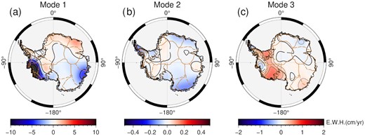
The rate maps of the trend components, Mode-1, Mode-2 and Mode-3 in Fig. 2.
The SCCs between the Mode-3 signal, and the ICE-5G and ICE-6G GIA models (Geruo et al. 2013; Peltier et al. 2018) are 0.692 and 0.691, respectively (Table 1), which imply a moderate-to-strong correlation between the Mode-3 signal and the GIA effect.
Spatial correlation coefficients between the GIA models and ICA spatial modes (95 per cent confidence level). The GIA-related modes are labelled in red.
| Mode-1 | Mode-2 | Mode-3 | Mode-4 | Mode-5 | Mode-6 | ||
|---|---|---|---|---|---|---|---|
| ICE-5G | −0.045 | −0.065 | 0.692 | −0.398 | −0.074 | 0.371 | |
| 2002–2020 | ICE-6G | −0.228 | −0.068 | 0.691 | −0.468 | 0.035 | −0.122 |
| ICE-5G | −0.064 | −0.058 | 0.624 | 0.087 | 0.252 | 0.462 | |
| 2002–2009 | ICE-6G | −0.157 | 0.180 | 0.469 | 0.338 | 0.112 | 0.434 |
| ICE-5G | −0.030 | 0.032 | 0.664 | −0.301 | −0.042 | 0.474 | |
| 2010–2020 | ICE-6G | −0.183 | 0.106 | 0.713 | −0.449 | 0.036 | −0.060 |
4.2 Periodic components
ICA also effectively separates the periodic components from the long-term components. Time-series IC4 and IC6 show periodic signals on different timescales. Mode-4 signal captures the mass loss along the west coast of the AP, which is concentrated along the larger glaciers (e.g. George VI). The corresponding IC4 time-series shows periodic signals at the 3–4-yr scale, which are probably related to periodic atmospheric and oceanic changes around Antarctica. Mode-6 signal shows mass gain that is distributed across the entire AIS, with the corresponding IC6 time-series possessing a cyclical signal with a 1-yr period. Mode-6 signal may be related to seasonal changes across Antarctica. Mode-4 and Mode-6 signals demonstrate that ICA can effectively separate periodic meteorological signals and long-term signals.
4.3 Independent events
ICA can also identify accidental independent events. In Mode-5, we found that there were two significant mass gain signals in East Antarctica, with the largest mass gain occurring in 2009 and the other in 2011. The temporal coincidence of these signals with the two extreme snowfall events in 2009 and 2011 that were reported by Boening et al. (2012) suggest a direct connection between the Mode-5 signal and snowfall events. The influence of anomalous snowfall events can also be found in other cyclical IC4 components. The strange variations around 2009 are considered to be driven by snowfall events.
We eliminate the impact of these events, and verify whether the remaining long-term ICA components, which should be temporally insensitive, can still be obtained by removing the January 2009–June 2010 period, dividing the remaining data set into two sections, and repeating the ICA for these two time periods.
The order of the ICA results may vary due to the different subintervals. We reorder the ICA results to align the components with similar information to those for the entire data set since the order of the ICA results does not represent the significance of each component. Furthermore, the fact that the different subintervals contain different information inevitably means the results from different subintervals may not be well aligned. The results of the former period (2002–2009) are shown in Fig. 5, with the corresponding time-series presented in Fig. 6, and the results of the latter period (2010–2020) are shown in Fig. 7, with the corresponding time-series presented in Fig. 8.
The first six ICA-extracted spatial modes for the former period (2002–2009).
Corresponding time-series of the decomposed spatial modes in Fig. 5.
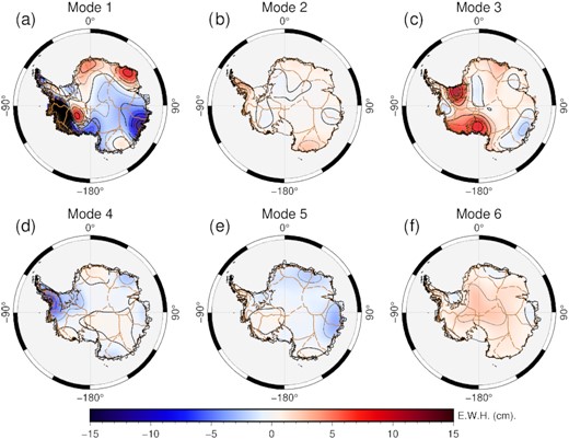
The first ICA-extracted six spatial modes for the latter period (2010–2020).
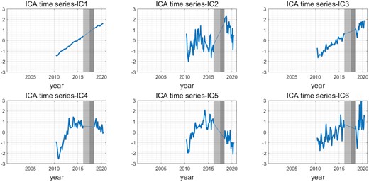
Corresponding time-series of the decomposed spatial modes in Fig. 6. The grey shading denotes the data gap in the study period, with the GRACE/GRACE-FO gap (July 2017–May 2018) in dark grey and the discarded period (July 2016–July 2017) in light grey.
The mass gain component in East Antarctica (Mode-5 in Fig. 2), which is related to snowfall events, is no longer detectable in the results for the two periods after excluding the period of detected snowfall events, as expected.
A comparison of the results from the different time periods indicates that most of the basic spatial patterns of the long-term components (Mode-1 and Mode-3) have remained. The differences in their spatial distributions reflect the development of the same components at different periods.
Many interesting local differences are observed in Mode-1 glacial component. Some notable glacial changes that have occurred since 2009, such as the expansion of the West Antarctica mass loss area, the onset of significant mass loss along Totten Glacier, East Antarctica and the onset of mass gain along Ice Stream C, West Antarctica, are identifiable (Fig. 7a).
The GIA related modes for two time periods (Mode-3 in Figs 5 and 7) show significant spatial differences between the former and latter periods (Figs 5c and 7c), even though the GIA-related mode is still detectable across both time periods. The former is primarily concentrated across MBL, whereas the latter is primarily distributed across the RIS and FRIS. These differences may be due to the averaging process when using SH coefficients from the three data centres.
We examine the SCCs between the ICA modes and GIA models (see Table 1) to determine the ability to extract the GIA signal via ICA. The results show that the SCCs for the GIA-related modes and models are 0.624 and 0.469 for the former period, and 0.664 and 0.713 for the latter period, respectively. Considering that the SCC between the ICE-5G and ICE-6G GIA models is 0.7023, it is reasonable to infer that the two spatial patterns may reflect the GIA signal.
5 CONCLUSION AND OUTLOOK
The ICA method was used to analyse AIS mass changes. Long-term components, periodic components at different timescales, and accidental events have all been successfully separated using ICA. This study has found that:
ICA can recognize and separate the signals from complex gravity changes. The overall mass changes of Antarctica can be decomposed into multiple statistically independent components, although each component still consists of a few physical processes.
The superposition of multiple long-term trends that originated from different physical processes can be decomposed into independent components. The Mode-3 signal showed a moderate-to-strong correlation with GIA.
The period of the used data set has the most direct impact on the ICA results. Rapid increases in snowfall in the late 2000s might have caused dramatic spatial and temporal changes, especially for the periodic components, which are associated with climate change.
A comparison of the results from two different time periods demonstrated that the long-term GIA trend could be obtained. The glacier-related component revealed an expansion of known mass loss areas, such as the AMS and Totten Glacier, after 2009.
Conversely, some of the expected important signals, such as precipitation, have not been separated, and are not presented in any of the results. Furthermore, the sICA results are mainly analysed in this study, even though we found the existence of annual, 3–4-yr, 5–6-yr and larger-scale AIS periodicities (Appendix B), and a possible association with ENSO via the tICA results. The combined use of different ICA methods should be considered in future studies.
The incorporation of different numerical models, such as regional atmospheric model (RACMO) and GIA models, is needed to better interpret the ICA results and relate them directly to physical processes. Furthermore, it is necessary to combine the ICA results with reanalysis data and multisource data, such as satellite altimetry, to extend the duration of the observations, which could enable us to better understand AIS changes and the AIS response to current climate changes over longer timescales. ICA is generally an effective approach to extract abundant information from a given data set without making any assumptions about the data, and can therefore help us to better understand what the data represent.
We propose the use of ICA in future GRACE/GRACE-FO studies that will attempt to elucidate GIA and other drivers that impact AIS mass changes.
ACKNOWLEDGEMENTS
The authors would like to thank NASA, JPL, CSR and GFZ for acquiring and providing the GRACE/GRACE-FO data. The authors are also grateful to J.V. Stone for providing the ICA algorithm and code. Generic Mapping Tools (Wessel et al. 2019) was used to produce the figures.
DATA AVAILABILITY
The GRACE and GRACE-FO data underlying this paper are available in The Physical Oceanography Distributed Active Archive Center (PO.DAAC). The ICA algorithm and code used in this paper are available from J.V. Stone, the source code author’s website (http://jim-stone.staff.shef.ac.uk/bss.html).
REFERENCES
APPENDIX A: DISCREPANCIES BETWEEN THE DATA SETS
We tested the different spherical harmonic coefficients provided by three data centres (CSR, GFZ and JPL) and their average. We first calculated the eigenvector spectrum for each data set via PCA (Fig. A1), which yielded accumulated variance ratio curves of the three individual data sets that were very similar. Each of the three data sets possess ratios above 0.7 for the first six components, with the JPL ratio being slightly higher than the other two, and the average (AVG) shows the highest ratios (even higher than that for each individual data set), with a ratio of about 0.75.
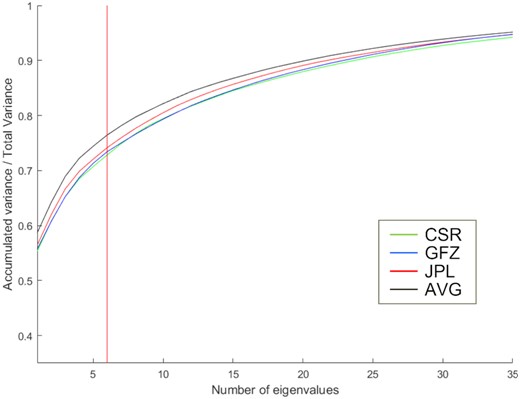
Accumulated eigenvalue spectrum derived from implementing PCA method on different data sets. Green, blue, red and black curves are for the CSR, GFZ, JPL and AVG (the average coefficients of the above three data sets) data sets, respectively. The red cut-off line indicates the first six eigenvalues that were selected.
We then used sICA separately for the different data sets, with the results shown in Figs A2 and A3. We find that the results for the dominated ice/snow signals in Mode-1 are identical across the data sets. There is also a good agreement among the data sets for the periodic variations of the Antarctic Peninsula in Mode-4 and the snowfall events in Mode-5. However, there are different biases among each of the data sets for some of the weaker signals. For example, although the additional linear trends associated with the GIA signal have been successfully separated for all of the data sets (Figs A3c1–c4), the corresponding spatial distributions differ widely (Figs A2c1–c4). Among these, the AVG and CSR results show a two-peaked spatial feature across FRIS and MBL, respectively, whereas GFZ and JPL show a single-peaked spatial feature. Furthermore, the spatial distributions of the remaining high-frequency meteorological signals also differ significantly (Figs A2f1–f4). This is potentially due to the large discrepancy in the minor signals after the PCA implementation in the first step. However, this could also be attributed to the signal mixing owing to incomplete decomposition. We therefore used the average solution of the three data sets, as mentioned in Section 3, to avoid any bias in the results.
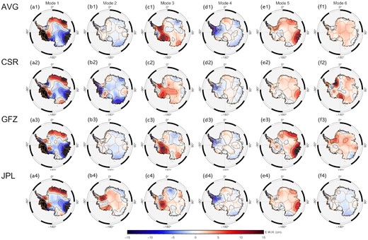
The first six spatial modes extracted via sICA from the AVG (average of three data sets), CSR, GFZ and JPL data sets.
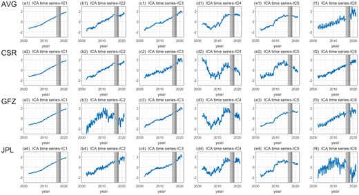
Corresponding time-series of the decomposed spatial modes extracted via sICA from the AVG, CSR, GFZ and JPL in Fig. A2. The grey shading denotes the data gap in the study period, with the GRACE/GRACE-FO gap (July 2017–May 2018) in dark grey and the discarded period (July 2016–July 2017) in light grey.
APPENDIX B: COMPARISON OF DIFFERENT ICA METHODS AND PCA
Different ICA methods can achieve different aspects of independence, as mentioned in Section 3. sICA maximizes the independence in the spatial domain, while tICA maximizes the independence in the temporal domain. Different ICA methods may be suitable for different scenarios; therefore, we tested three ICA methods, sICA, tICA and stICA, and compared their results with those of the classical PCA method to determine the most appropriate method for AIS studies. The results are shown in Figs B1 and B2.
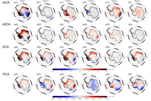
The first six spatial modes extracted via sICA, stICA, tICA and PCA. Note the different colour scales for the ICA and PCA results.
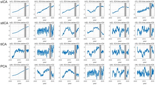
Corresponding time-series of the decomposed spatial modes extracted via sICA, stICA, tICA and PCA in Fig. B1. The grey shading denotes the data gap in the study period, with the GRACE/GRACE-FO gap (July 2017–May 2018) in dark grey and the discarded period (July 2016–July 2017) in light grey.
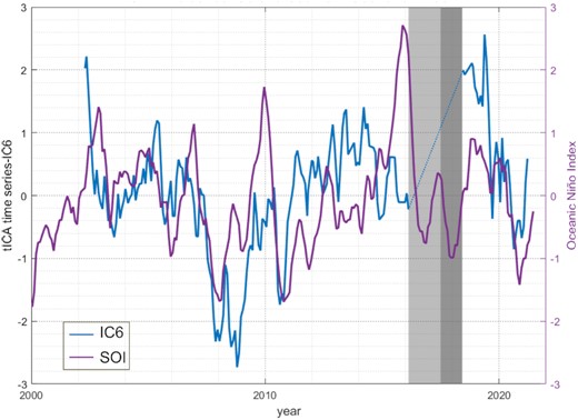
tICA time-series IC6 and Southern Oscillation Index The grey shading denotes the data gap in the study period, with the GRACE/GRACE-FO gap (July 2017–May 2018) in dark grey and the discarded period (July 2016–July 2017) in light grey.
We processed the data in the same way, with the first six components selected for each of the methods. Contrast to the sICA results in the Section 4, the six tICA spatial modes (Figs B1a3–f3) are extremely similar, while the corresponding time-series (Figs B2a3–f3) exhibit diverse periodicities at different timescales. The tICA results may represent AIS-scale characteristics over different periods. For example, IC1 shows a dramatic shift in the trend from 2003 to 2007, IC2 and IC3 clearly reflect annual AIS variations, and IC4, IC5 and IC6 exhibit potential periodic variations at 10+-, 3–4- and 5–6-yr timescales, respectively.
We particularly found that IC6 may be correlated with the Southern Oscillation Index (SOI, Fig. B3), which responds to the intensity of the possible El Niño-Southern Oscillation (ENSO) and La Niña activities. The overall trend and periodicity are well matched between SOI and IC6, with the exception of some degree of divergence in 2006 and 2016, which may demonstrate the tele-coupling of the AIS with ocean activity.
The stICA results can be considered a trade-off between sICA and tICA (Figs B1a2–f2 and B2a2–f2). stICA can effectively extract independent features in the temporal domain, such as IC2, IC5 and IC6, which are closer to the periodic signals that were separated via tICA than those that were separated via sICA. At the same time, more spatial details can also be obtained via stICA compared with tICA, such as the separation of the spatial features of the abnormal snowfall events across East Antarctica in Mode-2.
We also compared the ICA with the classic PCA method (Figs B1a4–f4 and B2a4–f4). The first six principal components of PCA accounted for 58, 5.5, 4.7, 3.3, 2.2 and 2.0 per cent of the total variation, respectively. The first component shows the dominant long-term trend of the AIS, whose spatial Mode-1 is almost identical to the regressed linear trend (Fig. 1). The second component exhibits long-period variations, with East and West Antarctica in an opposite phases. The third component shows mixed signals from the Antarctic Peninsula and Wilkes Land. The fourth component shows annual variations, while the fifth and sixth components show periodic variations at medium-term timescales. The PCA results are somewhat similar to the tICA results, in that they largely represent AIS-scale characteristics, which leads to a concise and clear time-series, whereas the spatial features are ambiguous and difficult to identify.
The most important difference between PCA and the three ICA methods is that PCA does not capture physical processes, such that each PCA component is a superposition of multiple physical processes. Therefore, it is impossible to extract independent physical processes of interest for a specialized study via PCA.
The GIA-related signal, which possess the largest uncertainty across the AIS, can only be effectively separated via sICA. We are also more familiar with some spatially distinct regions than the periodic time-series, such as the intense ice melting in the AMS and the snow accumulation in East Antarctica. Identifying these spatial features will help us relate the ICA results to specific physical processes more easily. Therefore, we prefer to use ICA by maximizing the independence on the spatial domain in this study, and will also consider the combination of other ICA methods for further comparisons with atmospheric models and reanalysis data in the future.
