


SUMMARY
We have formulated a 2-D Sn attenuation tomographic model to investigate the uppermost mantle shear wave Q and its tectonic implications beneath southeastern Tibet near Namche Barwa. To achieve our objective, we first compute interstation Q values using the two station method (TSM) analysis on 618 station pairs obtained from 26 regional earthquakes (Mw ≥5.5) with epicentral distances ranging from 5° to 15° recorded at 47 seismic stations belonging to the Namche Barwa network (XE network, 2003−2004). Furthermore, the QSn tomographic model is generated by utilizing these interstation Q values. QSn values are varying from 101 to 490 in the region. The tomography image reveals high attenuation (≤200 Q values) in the central region. Regions of low attenuation (>200 Q values) are observed in the southern part and in some small regions beneath the northern side of the study area. Consecutive high-low-high QSn values have been observed in the south part of the Lhasa block. The obtained QSn values, along with the prior isotropic Pn velocity model of the study area, indicate that the scattering effect is causing significant Sn wave energy dissipation due to structural heterogeneity present in the uppermost mantle beneath the region. This may be the result of the break-up of the subducting Indian Plate beneath the area.
1 INTRODUCTION
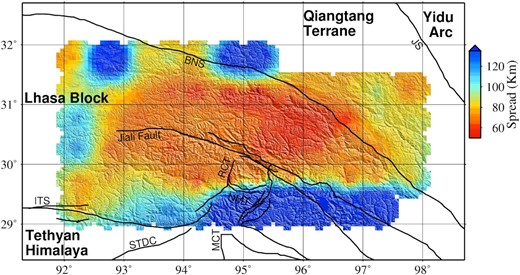
The Himalayan Mountain belts and Tibetan plateau are formed due to continuous continental collision of the Indian and Asian plates since the last 50 Ma (e.g., Molnar & Tapponnier 1975; Yin & Harrison 2000; Royden et al. 2008). The eastern end of the Himalayan orogenic belt is terminated by the Eastern Himalayan Syntaxis (EHS), marked by the changes in the strike of the geological units and structures (Fig. 1). The EHS is a manifestation of the deformation process(es) associated with the indenting corner of the Indian Plate and Tibetan plateau (e.g., Zeitler et al. 2001, 2014). It is a broad region of deformation and consists of the Himalayan Terrane, Lhasa block and Qiangtang terrane. At the surface, Indus-Tsangpo Suture (ITS) separates the Himalayan terrane from the Lhasa block, while Bangong-Nujiang Suture (BNS) separates the Lhasa block from the Qiangtang terrane (Fig. 1). The Namche Barwa Complex (NBC), the core part of the EHS, has a distinct signature from the surrounding area. It is a tectonically active area characterized by highly deformed metamorphic rocks (from granulite to amphibolite facies) bounded by thrust and strike-slip faults (Booth et al. 2004, 2009; Zeitler et al. 2014). The western margin is modified by the Rong Chu shear and fault zone, while the Nam-la thrust modifies the southern and southwestern parts of the NBC (Fig. 1). The Jiali fault zone flanks the northern portion of the NBC region. It is a dextral strike-slip fault oriented in a SE−NW direction, accommodating the clockwise rotation around syntaxis (Armijo et al. 1989; Burg et al. 1998). The EHS spatially shows a transition from convergent and extensional tectonics in the west to the strike-slip transition in the east.
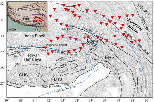
The figure shows the tectonic map of southeastern Tibet. Red inverted triangles denote the deployed seismic stations of the Namche Barwa seismic network. Only the electronic edition contains the colour version of this figure. STDS, South Tibetan Detachment System; LHS, Lower Himalaya Sequence; GHS, Greater Himalaya Sequence; RCT, Rong Chu Thrust; NMT, Nam-la Thrust; GP and NB, Gyala Peri and Namche Barwa Peaks.
Various geological (e.g., Ding et al. 2001; Xu et al. 2012; Zeitler et al. 2014), seismological (e.g., Sol et al. 2007; Fu et al. 2010; Zhao et al. 2013; Singh et al. 2015; Tiwari et al. 2017) and geodetic (e.g., Gan et al. 2007; Sol et al. 2007) measurements have been used to investigate the EHS and the surrounding southeastern Tibetan plateau in order to unravel the tectonics of the region. However, the geodynamic process responsible for the south-east expansion and deformation is still unclear and remains debatable. Gravity (Jiménez-Munt et al. 2010), body wave tomography (Tilmann et al. 2003; Zhou & Murphy 2005), Pn velocity (McNamara et al. 1997; Liang & Song 2006; Hearn et al. 2019), shear wave splitting (Huang et al. 2000; Sol et al. 2007; Chen et al. 2010), and receiver function (Kind et al. 2002) studies all strongly suggest that southern Tibet is underlain by relatively colder and more rigid Indian continental lithosphere, possibly extending past the BNS. The mid-to-lower crustal flow (e.g., Clark et al. 2005; Royden et al. 2008) and Vertical Coherent Deformation (VCD) of the crust and lithospheric mantle (e.g., Sol et al. 2007; Bendick & Flesch 2007) are the two most popular models for the internal deformation to understand the expansion mechanism beneath southeastern Tibetan plateau. The difference between these two models is in (de)coupling of crustal and lithospheric materials. Dong et al. (2016) produced an extensional extrusion model for the region based on their recent magnetotelluric analysis. According to them, the southeastward expansion results from an accumulated series of east-west ductile extension zones. These contradictions in geodynamic models imply that no single model can explain all these deformation scenarios of the region. Hence, a newer study of the crust and uppermost mantle is required to comprehend the region's actual deformation process(es).
Attenuation characteristics of regional seismic phases (e.g., Lg, Pg, Sn, and Pn) can provide information about the rheology beneath a region (e.g., Ni & Barazangi 1983; Mitchell et al. 1997; Sandvol et al. 2001; Singh et al. 2011; He et al. 2017; Singh et al. 2019b). Spatially, intrinsic attenuation is the indicator of temperature variation, especially at mantle conditions, whereas the seismic velocity is sensitive to both temperature and compositional variation. Therefore, attenuation (Q−1) studies can help in distinguishing compositional and temperature anomalies in the uppermost mantle. It can also provide important constraints regarding the lithospheric architecture and geodynamics of an area (e.g., Sheehan et al. 2014). Lg and Pg phases are sensitive to crustal thickness as well as crustal deformation and rheology (e.g., Xie et al. 2004; Singh et al. 2012; Zhao et al. 2013, 2015; Singh et al. 2019b; Jaiswal et al. 2020), while Sn and Pn phases are sensitive to mantle lid deformation and rheology (e.g., Sandvol et al. 2001; Al-Damegh et al. 2004; Gök et al. 2003).
The Sn phase was chosen to investigate uppermost mantle attenuation instead of other regional phases because it is more sensitive to partial melting and temperature change underneath an area. It is a high-frequency regional seismic phase that travels through the uppermost mantle above the asthenospheric low-velocity layer. Therefore, spatial Sn phase attenuation plays a vital role in imaging the deformation and tectonics of the uppermost mantle (e.g., Molnar & Oliver 1969; Barazangi & Isacks 1971). The recorded Sn signals are sensitive to velocity gradient and attenuation in the uppermost mantle (Ni & Barazangi 1983). It travels through both the continental and oceanic lithospheric mantles. It has a typical period of 0.5 to 2 sec. Huestis et al. (1973) observed that the typical Sn phase travels at a velocity of 4.3 to 4.7 km/sec.
Studies on the attenuation characteristics of Lg and Pg waves have been done in the past to find the crustal tectonics of the Tibetan Plateau (e.g., Xie 2002; Fan & Lay 2003a, b; Xie et al. 2006; Bao et al. 2011a; Fisk & Phillips 2013; Zhao et al. 2013; Singh et al. 2015, 2019b; Jaiswal et al. 2020). Some studies on Sn propagation efficiency (Ni & Barazangi 1983; McNamara et al. 1995; Barron & Priestley 2009) have also been conducted to find the propagation characteristics within the uppermost mantle beneath the Tibetan plateau. However, no high-resolution Sn attenuation tomography has been attempted for the Tibetan plateau, which is of utmost importance for understanding the deformation and rheology of the uppermost mantle beneath the region. This study focuses on the southeastern part of Tibet. The primary objective of this study is to find the uppermost mantle attenuation structure beneath the region to understand the geodynamic architecture of the EHS. First, to achieve this objective, interstation QSn values are obtained using the two station approach of Zhao et al. (2015). Secondly, the singular value decomposition (SVD) algorithm is used to obtain a 2-D attenuation tomographic image using the above interstation QSn values. Our inferred attenuation structure adds new constraints to the composition and thermal structure of the uppermost mantle beneath southeastern Tibet.
2 DATA AND METHODS
2.1 Used data and pre-processing
We used Sn-phase waveform data from 47 seismic stations of the XE network (Namche Barwa project). This network was operated during the years 2003 to 2004 (Meltzer 2003; Sol et al. 2007), covering the Himalayan terrane, the Lhasa block, and the Qiangtang terrane of southeastern Tibet. The events used in this analysis are located between 5° and 15° epicentral distances to ensure only the first arrival and fully developed S signal. For selecting the lower limit of epicentral criteria, we calculated the Sn phase crossover distance for our region using an earth model with a crustal thickness of 70 km and average crust and mantle shear wave velocity of 3.75 and 4.50 km s–1, respectively. 4.2° is the corresponding crossover distance. To avoid ambiguity, we set the lower bound limit at 5° to remove the Pg and Sg phases and ensure that only the first S-arrival signal is present. The straight portion of the shear wave velocity in the travel time curve is used to set the upper limit of the epicentral distance (15°, e.g., Pei et al. 2007). A fully developed Sn phase may not be observed in the Sn velocity window after this distance. Furthermore, energy from the upper mantle discontinuities can arrive with significant amplitude within the velocity window of the Sn phase.
We further restricted the events by selecting only those events that have magnitude ≥5.5 to ensure high-quality Sn waveforms. All the earthquakes used in the present study are of crustal origin. Since, the Sn phase is an uppermost mantle refracted phase, the events that originated within the crust can be used to map the uppermost mantle (Fig. 2). All seismic waveforms were visually inspected to avoid the inclusion of any noisy signals. Following this pre-processing, 845 high-quality waveforms were retained from the 47 seismic stations. The instrument responses were removed from the original seismograms to avoid any potential bias of different types of seismic stations.
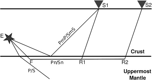
The cartoon illustrates the simplified concept of the two station method, as well as source-to-receiver ray paths of Sn and other phases.
To inspect the Sn phases, we rotated the vertical, E−W and N−S components of the seismogram into the vertical, radial and transverse components. The radial component contains P and SV phase energy, while the transverse one is predominated by SH phase energy. Each seismogram was visually examined for the presence of the Sn phase on the vertical, radial and transverse components. However, in all cases, we prefer the transverse component because the shear wave is clearly visible on it and it is less influenced by the P-wave coda (Wei et al. 2018). The Sn velocity is generally between 4.3 and 4.8 km s–1 (e.g., Huestis et al. 1973; Bao et al. 2011b; Barron & Priestley 2009; Mousavi et al. 2014). The average velocity of Sn phase in our study region is 4.5 km s–1 (Fu et al. 2010; Lü et al. 2013). The waveform data was bandpass filtered between 0.1 and 5 Hz, to enhance the amplitude of Sn phase. Following filtering, the signal-to-noise ratio (SNR) analysis was performed to ensure high-quality waveforms for regional Q estimation, which is also a qualitative approach for the Sn phase propagation efficiency. For that, we calculated the maximum spectral amplitude within the defined Sn velocity window (4.1−4.8 km s–1) as the signal and the root mean square amplitude of the Pg window (5.2−6.1 km s–1, Bao et al. 2011b; Singh et al. 2019b) as the noise. We selected only those waveforms that have SNR = [Sn/rms(Pg)] ≥ 2. These waveforms were further visually checked for the presence or absence of Sn phases. To check the propagation efficiency of the Sn phase from the event to the station, we filtered the seismograms in low (0.1−0.5 Hz) and high (0.5−2 Hz) frequency ranges and checked the waveforms in both frequency ranges on the radial, transverse and vertical components. We categorized the propagation efficiency as ‘efficient Sn’, ‘inefficient Sn’ and ‘blocked Sn’ based on the presence of Sn phase in both frequency domains. If the Sn phase is clearly seen in both frequency domains, the phase is efficiently propagating through the region. If the Sn phase is seen in the high-frequency range but not distinguishable or absent in the lower frequency range, the Sn phase is propagating inefficiently through the region. If the Sn phase is invisible in both frequency ranges, the phase propagation is blocked across the area. Fig. 3 shows the transverse component waveforms at various stations in the low and high-frequency domains for three different events. The presence of efficient, inefficient, and blocked Sn waveforms is depicted in the figure. We have efficient Sn waveforms from events coming from the Xizang and Indo-Bangladesh region, while the waveforms from the Yunnan event have inefficient and blocked Sn (Fig. 3). We selected only efficient and inefficient Sn waveforms for the quantitative Q measurements. We included only those events that have been recorded at a minimum of four stations. Fig. 4 shows the Sn propagation efficiency map of the region.
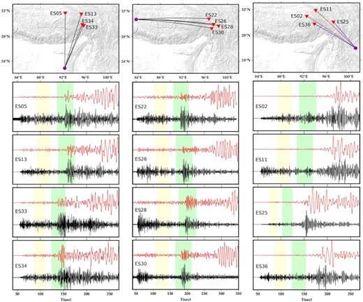
The figure shows examples of efficient, inefficient, and blocked Sn waveforms. It depicts the transverse component waveforms in the low (0.1−0.5 Hz) and high (0.5−2.0 Hz) frequency ranges at each station coming from the Indo-Bangladesh border, Lhasa terrane and Yunnan province. The waveforms in red and black represent low and high-frequency filtered waveforms, respectively. Light yellow and green colours represent the Pg time window (5.2−6.1 km s–1) and Sn time window (4.1−4.8 km s–1), respectively. Seismic stations and events are depicted by yellow inverted triangles and purple circles. The ray paths in black, brown, and blue colour represent efficient, inefficient and blocked waveforms, respectively. Only the electronic edition contains the colour version of this figure.
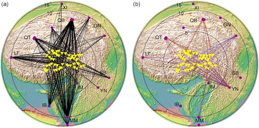
The map shows the Sn ray paths with their propagation efficiency and epicentral distribution (5−15°) of the events used in the study. Yellow inverted triangles and purple circles show the location of seismic stations and used events. (a) Black ray paths denote the efficient Sn, (b) Brown and blue ray paths denote the inefficient and blocked Sn phases, respectively. Only the electronic edition contains the colour version of this figure. GN, Gansu; IB, India-Bangladesh Border; IM, India-Myanmar Border; LT, Lhasa Terrane; MM, Myanmar; QB, Qaidam Basin; QT, Qiangtang Terrane; SB, Sichuan Basin; XI, Xinjiang; YN, Yunnan.
We considered both efficient and inefficient Sn phase vertical component waveforms with clear Sn marking for the Sn amplitude spectrum analysis. The Sn waveforms were extracted using a group velocity window of 4.1−4.8 km s–1 and the noise time series were collected from an equal length window as the Sn phase before the first arriving P wave. The signal (Sn) and noise (pre-Pn) amplitude spectra are then computed using the fast Fourier transform technique. We used a 15 per cent cosine taper in order to avoid spectral leakage. The cosine taper is preferred because it smoothly decays the data to zero at the beginning and end of the signal and noise time window without significantly changing the Fourier transform of the signal and noise time window. At this stage, we have again performed SNR calculation and selected only those portions of the spectra that have SNR ≥ 2. Only the SNR ≥ 2 part of the Sn amplitude spectra is further used in the two station method (TSM) technique (Zhao et al. 2015) to find the interstation uppermost mantle attenuation. After computing the corrected Sn spectra, we started the station pairing process. We select only those station pairs that have an interstation distance ≥150 km to avoid uncertainty in interstation QSn measurement.
2.2 Two station method
In this study, the two station approach of Zhao et al. (2015) is used to investigate the interstation QSn value. The method computes the spectral amplitude ratio of waveforms recorded at two given stations by an event followed by calculating the interstation QSn value. In the TSM technique, events and stations are arranged in such a way that the source and stations are aligned along the great circle path, or that the azimuth between a given source and two stations should be ≤15° (Xie et al. 2004; Zhao et al. 2015).
The right-hand side of this equation is known as the reduced spectral ratio. It is a mathematical term that is commonly used in Q tomography. The equation is a straight-line equation in the logarithmic domain that can be used to calculate Q0 and η value from a plot of reduced spectral ratio and frequency.
Fig. 5 shows an example of the TSM technique for obtaining the interstation Q0 value for station pair ES38−ES09 for an event. Sn amplitude and noise spectra from the same earthquake are plotted at stations ES38 and ES09 for the windowed signal and noise with a 15 per cent cosine taper. Fig. 5(c) depicts the computation of the QSn and η values from the logarithm plot of reduced spectral ratio and frequency. In practice, the event and stations are not aligned along the great circle path and are at a certain angle. In such cases, the estimated Q0 could be inaccurate because of the non-isotropic source of radiation and attenuation outside the great circle path (Xie et al. 2004). To reduce this, we only allowed station pairs with a maximum azimuth of 15° between the source and two stations (Xie et al. 2004; Zhao et al. 2015). The interstation distance is another crucial parameter that can cause the potential error in QSn measurements. We chose station pairs with a minimum interstation distance of 150 km. Following these selection criteria, we calculate the standard error to check the reliability of the obtained QSn measurements (He et al. 2017). It denotes the standard deviation of the estimated mean Q value. We retained only those Q measurements that have ≤20 per cent error. After the error estimation process, 618 station–station QSn values were retained and used in the tomographic computation.
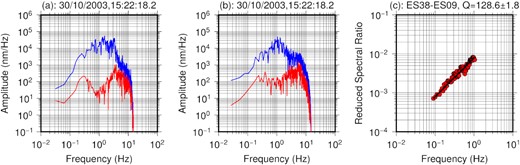
Panels (a) and (b) show the Sn amplitude spectra (solid blue line) and noise (solid red line) for stations ES38 and ES09, respectively, for the same earthquake whose origin time is marked at the top of each panel. Panel (c) shows the reduced spectral ratio versus frequency plot to obtain the Q0 after the TSM analysis. The top of the panel shows the station pair ES38−ES09 and the Q0 value. The Q0 value is obtained through linear regression fitting. Only the electronic edition contains the colour version of this figure.
2.3 Tomography
3 RESULTS
Initially, 618 interstation QSn values are obtained for the region using the TSM technique. The ray paths of these station pairs are plotted in Fig. 6. We observe dense ray paths throughout the region except at side-boundaries. These interstation QSn values are then used to perform QSn tomography. In order to find a reliable shear wave attenuation scenario for the uppermost mantle of the region, the selection of an optimum α and λ (eq. 9) is essential to suppress the solution instability caused by heterogeneity in data coverage.
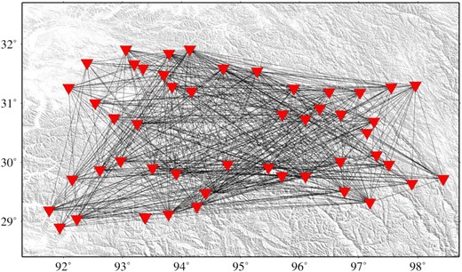
The figure shows the interstation ray paths coverage map of the study area. Following the TSM analysis, we have a total of 618 interstation ray paths. Only the electronic edition contains the colour version of this figure.
The optimum value of λ is determined by plotting the percentage of smaller 1/Q values (1/Q ≤0.001) obtained from the tomography process with varying λ for different values of α (Fig. 7a). Smaller 1/Q values are generally physically impossible model grid values (Nolet 2008) that act as artefacts in the final model. When λ is greater than 2.6, most of the models have ≤4 per cent smaller 1/Q values for the majority of α values. As a result, 2.6 was chosen as the optimum λ value. For this optimum λ value, an L-curve is plotted between the model norms and the data residuals for different values of α to find the optimum α (Fig. 7b). We used the maximum curvature method to find the optimum α. The obtained optimum α (1.4) is marked by a red star in Fig. 7(b).
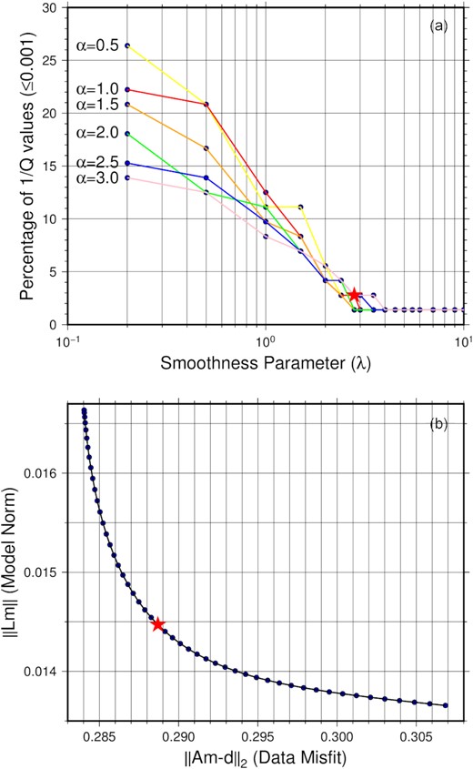
(a) Percentage of 1/Q (≤0.001) plot with varying smoothing parameters (λ) for different values of damping parameter (α). The red star denotes the optimum λ. (b) Plot of the L-curve between the model norm and the data misfit for the obtained optimum λ and with varying α. The trivial α values range from 0.1 to 5 with an increment of 0.1 interval. The optimum α is marked with the red star, which was obtained by using the curvature method. Only the electronic edition contains the colour version of this figure.
3.1 QSn tomography model
The 2-D QSn tomographic model for the region is obtained using 618 interstation Q values for the selected optimum values of α (1.4) and λ (2.6) (Fig. 8). QSn values vary from 101 to 490 in the region. To investigate the uppermost mantle attenuation scenario, the study area is divided into zones based on the obtained QSn values, namely low (Q ≤ 200) and high (Q > 200). The tomography image shows low QSn values in the central area (A). Regions of high QSn values are observed along the northern side of ITS (B) (southern portion of the study area) except in the central region. Some patches of high QSn are also observed in the north portion (C) of the study region. Consecutive high-low-high QSn patterns in the southern part of the study area provide insight into the breakage of the subducted Indian Plate beneath the central region. Low QSn values beneath the central region indicate scattering caused by structural heterogeneity in the uppermost mantle. The heterogeneity may be the result of the fragmentation of the underthrusted Indian Plate beneath the Namche Barwa area. It is worth noting that at the western end of our model area, there is some correlation between Pn velocity and QSn estimates. This might suggest that although scattering is the dominant mechanism for Sn phase attenuation, there is some evidence of intrinsic attenuation at 92°E to 93°E.
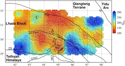
The map shows the 2-D Sn attenuation tomography of the region. The model is obtained at a 1 Hz reference frequency with a grid size of 0.5° × 0.5°. Grids with unreliable spread function and model covariance matrix are not shown in the QSn tomography. Only the electronic edition contains the colour version of this figure.
3.2 Spread function and uncertainty estimate
We used statistical measures to assess the reliability of the obtained QSn model. The SVD algorithm has the advantage of quantitatively measuring the Rm and Cm of the obtained QSn model when solving the damped least square tomographic inversion problem with damping and smoothness constraints. The Rm calculates quantitatively how any true tomographic model element is related to an estimated model using a smearing (weighting) process (Menke 2012). Smearing causes limited lateral resolution of the model that is given by spread function (SF). The SF ranges from 49 to 287 km. The obtained SF tomographic image (Fig. 9) suggests higher lateral resolution (low spread function, 49–80 km) in the central region, which is equivalent to our grid size (∼50 km). Some pockets of higher SF values (Fig. 9) are obtained along the region's boundaries. This may be because of the poor ray path coverage along the boundaries. The Cm represents the uncertainty measure of the estimated model (Aki & Richards 1980). The square root of the diagonal elements of the Cm is the measure of standard deviation. We obtained the tomographic relative uncertainty map for the region by using the Cm (Fig. 10). The relative uncertainty in 1/Q measurements varies from 1.0 to 2.7 throughout the study region. Lower uncertainty values are obtained throughout the study region, with some patches of relatively higher uncertainty obtained near the outer boundary of the study region (Fig. 10).
The spread function map of the region, which provides an approximate lateral resolution for the obtained QSn tomographic model. The Backus–Gilbert approach is used to calculate the spread function in order to determine the smearing distance caused by the resolution matrix (Rm). The colour scale is in km. Only the electronic edition contains the colour version of this figure.
![The relative uncertainty [δ(1/Q)/(1/Q)] map of the region depicts the uncertainty scenario in the obtained 1/Q tomographic model. δ(1/Q)/(1/Q) is derived from the model covariance matrix (Cm). The colour scale is expressed in percentage. Only the electronic edition contains the colour version of this figure.](https://oup.silverchair-cdn.com/oup/backfile/Content_public/Journal/gji/228/2/10.1093_gji_ggab380/1/m_ggab380fig10.jpeg?Expires=1750232392&Signature=vHTm3Um5NTNbQ1HWgRbjhnkhybUSpx7RYogt3AITZ93VFCHLpmpux23zrANrQFQAwNwW7GkGHeN1UIVFwrCVIMSMItyhgAqtp1ER4ORwWJUMHlTnEBwmWjF0ghsK8u0CKycuYE1Oxhy6gr0Pop3kN15b1s4pyQquzXqHOV9CL0qD2oI4uCDExjLDwLZYi7NRjSvcA4k40YdYAF7IvZIMJyr9eoEL4g7pUpYuSTWJO7RzdebXWkScWjAopbRMkunb0iI4Wn4FLWLK-Vya7-6W9rTfvAeTvDcgA8wtGS2dg3bhzN3tufMW~cyLjWiOsv9~AwHu5f~G40VYwPaHdJ-LkA__&Key-Pair-Id=APKAIE5G5CRDK6RD3PGA)
The relative uncertainty [δ(1/Q)/(1/Q)] map of the region depicts the uncertainty scenario in the obtained 1/Q tomographic model. δ(1/Q)/(1/Q) is derived from the model covariance matrix (Cm). The colour scale is expressed in percentage. Only the electronic edition contains the colour version of this figure.
In addition to the spread function, we performed checkerboard resolution tests at a grid size of 0.5° × 0.5° to cross-validate the reliability of the obtained tomographic model. The checkerboard resolution test used the synthetic model and the same experimental setup (ray path coverage and regularization parameters) as used to find the final QSn tomography of the region. We used two synthetic checkerboard models for the resolution tests. The initial synthetic model was built with a high Q value of 400 for even grids and a low Q value of 100 for odd grids. The second one is the synthetic model with 15 per cent Gaussian noise in the first synthetic model. Both synthetic checkerboard models were inverted, and the results are shown in Fig. S1. Checkerboard patterns were fully recovered across nearly the entire study zone, with the exception of a few spots near the south and north edges. Except in the south, where the checkerboard test revealed a higher resolution, the checkerboard test and spread function map are identical. Both strategies, however, have drawbacks.
4 DISCUSSION
4.1 Sn propagation efficiency
Several studies have previously been conducted to ascertain the Sn propagation characteristics of the uppermost mantle beneath the Tibetan plateau (Ni & Barazangi 1983; McNamara et al. 1995; Barron & Priestley 2009). The majority of them were of low resolution (Ni & Barazangi 1983; McNamara et al. 1995). Barron & Priestley (2009) investigated the efficiency of frequency-dependent Sn propagation across the Tibetan plateau. High-resolution models were produced using a large number of earthquakes providing dense ray paths and better azimuthal coverages. It was observed that, at lower frequency (∼0.2 Hz), Sn waveforms efficiently propagate through the entire plateau, but at higher frequency (∼1 Hz), they are either inefficiently propagated or blocked for the northern Tibetan plateau (Barron & Priestley 2009). Similar results were also reported by Ni & Barazangi (1983) and McNamara et al. (1995). These propagation studies have a low resolution in the study region because of the unavailability of seismic data. This study provides a high-resolution image of the Sn propagation efficiency beneath the EHS and surrounding regions, which was lacking in earlier studies (Ni & Barazangi 1983; McNamara et al. 1995; Barron & Priestley 2009).
Efficient Sn propagation is observed beneath the EHS and surrounding regions (Fig. 4a). Sn phase efficiently propagates through the uppermost mantle beneath most of the region where the waveform follows a continental path. Its transmission is not much affected by major tectonic boundaries, suture zones and physiographic divisions. Efficient Sn propagation characteristics for the majority of event-station pairs suggest a positive shear wave velocity gradient in the uppermost mantle, which may indicate a thicker upper mantle lid (Barron & Priestley 2009). Sn phases have been found to be blocked or inefficiently propagated for events originating in the Qiangtang terrane and Qaidam Basin. We have also observed inefficient Sn propagation from the western Yunnan province, which has lower mechanical rock strength and a mechanically decoupled crust and upper mantle (e.g., Sol et al. 2007). Inefficient Sn propagation has been observed primarily within a basin, sediment-dominated belt, or volcanic region, indicating the presence of a thin lithospheric mantle lid between the event station pairs (e.g., Ni & Barazangi 1983; Gök et al. 2003; Barron & Priestley 2009).
4.2 QSn tomography model and its significance
The spatial variation of the attenuation characteristics using the Sn phase reflects the uppermost mantle rheology of the region. The obtained QSn tomographic model shows low QSn values beneath the central part of the study region. High QSn values are mostly concentrated on the southern side of the study area. The observed apparent QSn values beneath the region are the combined contribution of the intrinsic and scattering attenuation. The intrinsic attenuation may be caused by temperature, partial melting and the presence of fluids beneath the region (e.g., Aki 1980; Fehler et al. 1992), while scattering attenuation is caused by heterogeneity beneath the medium (e.g., Lay & Wallace 1995; Sato et al. 2012). The apparent QSn beneath the region is frequency dependent. The frequency-dependent parameter (η), together with Q value, signifies the relative intrinsic and scattering attenuation beneath the region, but it is qualitative in nature. In general, high η values indicate scattering attenuation, while low η values indicate intrinsic attenuation (He et al. 2017). η values are varying from 0.1 to 1.5 in the region. Seismologists (e.g., Hoshiba 1991; Fehler et al. 1992; Mukhopadhyay & Tyagi 2008; Singh et al. 2016, 2017a, b; Biswas & Singh 2019; Singh et al. 2019a) quantified the relative contributions of intrinsic and scattering attenuation using the Swave and coda wave and discussed their role in understanding the material property and tectonics of the region. However, the quantification of intrinsic and scattering attenuation is beyond the scope of our study with the current data set.
The QSn variation is highly influenced because of the hot lithospheric mantle, heterogeneity, presence of partial melts and the absence of the uppermost mantle lid beneath the region (Sandvol et al. 2001; He et al. 2017). The observed consecutive high-low-high QSn values in the southern part of the study area may suggest that the breakage of subducted Indian Plate beneath the central region. The high-resolution body wave tomography models (e.g., Ren & Shen 2008; Zhang et al. 2012; Liang et al. 2012, 2016; Peng et al. 2016) also suggest the presence of fragmented Indian lithosphere beneath the region. The correlation between QSn and uppermost mantle velocity provides an important constraint on the thermal and compositional origins of seismic anomalies beneath the area (Romanowicz 1994; Artemieva et al. 2004). Pn and Sn propagations show a complex velocity distribution about the uppermost mantle structure in the study area (Liang & Song 2006; Pei et al. 2007; Lü et al. 2011, 2013; Li & Song 2018; Hearn et al. 2019). Earlier Pn velocity tomography (Liang & Song 2006; Lü et al. 2011) and Sn velocity tomography (Lü et al. 2013) of the Tibetan plateau suggest relatively low velocity beneath southeastern Tibet. However, these tomography models were of low resolution and lacked the XE network data set. In contrast, recent high-resolution Pn velocity tomography of the Tibetan region (Li & Song 2018; Hearn et al. 2019) suggests that Pn velocity is higher beneath southeastern Tibet. The high-resolution Pn velocity tomography of Hearn et al. (2019) suggests depth-dependent Pn velocity variation beneath the area. Fig. 11 shows a comparative model of the obtained QSn values and Pn velocity tomography (Hearn et al. 2019) for the study region. The model depicts a positive correlation between Pn velocity and Q measurements beneath the western portion of the study area; however, a negative correlation is observed between Pn velocities and Q measurements beneath the central and eastern study regions (Fig. 11). This could be due to the relative dominance of the scattering attenuation or the presence of melts in the uppermost mantle beneath the study area. Scattering attenuation accounts for the redistribution of seismic energy into different directions due to structural heterogeneity in the medium. Fragmentation of the underthrusting Indian Plate is likely to be responsible for some of the structural heterogeneities in the uppermost mantle resulting in the material property change that leads to scattering attenuation. The strength of the amplitude/energy decay depends on the material properties. On the other hand, the presence of the fragmented Indian Plate in the mantle lithosphere could explain the higher Pn velocity (Ren & Shen 2008). Theoretical observations from surface wave studies also indicate that the heterogeneity may increases the phase velocity of the surface wave (e.g., Samuelides & Mukerji 1998; Kumari et al. 2016; Dewangan & Sahu 2017). As a result, there is a generally negative correlation observed in the case of heterogeneity across the study region. Fig. 12 shows the QSn results along an E−W profile, as well as a simplified geodynamic model of the lithospheric mantle beneath southeastern Tibet. The model is redrawn and a simplified version of observations made in the tomographic images of Peng et al. (2016) are used. These images are consistent with the break-up of the underthrusting Indian Plate beneath the central area (Namche Barwa metamorphic massif) of the EHS, which is responsible for structural heterogeneity in the uppermost mantle beneath the area. It is the genesis of the lower QSn values in the central part of the EHS, as shown in Fig. 11.
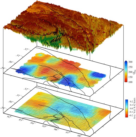
The block diagram depicts a comparison of QSn values (present study) and Pn velocity (Hearn et al. 2019) of the study area. The top one shows the tectonic and topographic map of the study area along with the location of the seismic stations. The red circle denotes the location of the seismic station. The velocity data is taken from Hearn et al. (2019) Pn velocity tomography for the distance range of 1000−1600 km. Only the electronic edition contains the colour version of this figure.
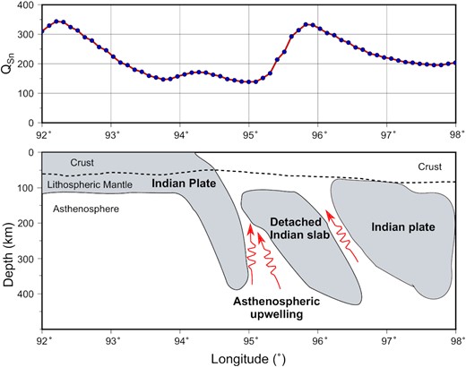
The cartoon illustrates the 2-D−QSn model (modified after Peng et al. 2016) for the west to east longitudinally traversing profile along 29.5°N latitude, together with QSn values. Only the electronic edition contains the colour version of this figure.
The Tibetan lithosphere around the EHS experiences E−W or NNE−SSW compressional stress and perpendicular extensional strain. These unequal extensions are the result of significant changes in the subducting direction around the intending corner of the EHS (Ren & Shen 2008; Liang et al. 2012; ; Liang et al. 2016; Zhang et al. 2012)), which may have resulted in the breakage or tearing of the Tibetan lithosphere–asthenosphere boundary (LAB) and the creation of a slab window beneath the region. Localized asthenospheric upwelling through the slab window, thermal erosion, and shear heating are responsible for the delamination of the lithospheric mantle beneath the area. The hotter asthenosphere is now in direct contact with the subcontinental lithospheric mantle, causing the partial melting of metasomatized peridotites. This is because peridotites have a lower solidus than asthenospheric temperatures (Williams et al. 2004; Ren & Shen 2008). Southern Tibet geochemical analysis reported partial melting of metasomatized peridotite in the spinel stability field (65−80 km, Williams et al. 2004). Geochemical and geochronological analysis (Burg et al. 1998; Ding et al. 2001; Zeitler et al. 2001; Booth et al. 2004, 2009) have also reported partial melting beneath the Namche Barwa area of the EHS. However, these studies have not specified the depth range of the partial melting beneath the region.
The EHS is a complex and highly deformed region formed by the continued collision of Indian and Asian plates. At the surface, the Indian Plate is supposed to be extended at least up to the ITS that connects the Himalayan Unit and the Lhasa Block (Zeitler et al. 2014). Gravity (Jiménez-Munt et al. 2010; Wang et al. 2019), body wave tomography (e.g., Tilmann et al. 2003; Peng et al. 2016; Liang et al. 2016), Pn velocity (McNamara et al. 1997; Liang & Song 2006; Li & Song 2018; Hearn et al. 2019) and receiver functions (Zurek 2008; Xu et al. 2013; Wang et al. 2019) studies all strongly suggest that southeastern Tibet is underlain by relatively colder and more rigid Indian continental lithosphere, which may extend to the BNS; however, the fate of the Indian crust and mantle lithosphere underneath the EHS region is still up for debate. Our QSn tomography model also is consistent with the northern extension of the underthrusting Indian Plate underneath the EHS. The observed high QSn values in the southern portion of the study region reflect that the Indian Plate extends to the middle of the Lhasa block in the mantle lithosphere. However, the distinctive spatial variation of QSn values in the study region has not been observed, indicating gaps in the Indian Plate in the central part of the study region.
Except for a few small regions with high QSn values, low QSn values dominate the northern portion of the study region. Higher temperatures, partial melting, and structural heterogeneity in the mantle lithosphere underneath the location could explain the low QSn values. The Asian Plate lies beneath the northern portion of the study region. According to the S-to-P receiver function study of southern Tibet (Xu et al. 2013), the spatial variation is not continuous, and there is a gap in the LAB underneath the central part of the study region. If the gap in the LAB is the only factor responsible for the attenuation and velocity, the seismic anomaly is of thermal origin. Low QSn and low Pn velocity is expected to be observed in this case, which could be caused by higher temperature, partial melting, and fluids. On the other hand, as illustrated in Fig. 12, higher Pn velocity is reported in the uppermost mantle underneath the central region (Hearn et al. 2019). This rules out the possibility of the seismic anomaly being of thermal origin. It further indicates a non-uniform LAB gap and fragmented Indian Plate underlying the study region, which acts as the primary source of structural heterogeneity, accounting for the observed low QSn values (this study) and reported high Pn velocity (Hearn et al. 2019).
Several seismic attenuation studies (e.g., Fan & Lay 2003b, a; Xie 2002; Xie et al. 2006; Zhao et al. 2013; Singh et al. 2015; Jaiswal et al. 2020) were conducted using Lg data to find the crustal rheology and tectonics beneath the Tibetan plateau. Their results suggest the partial melting or existence of a localized or continuous crustal channel flow beneath the Tibetan Plateau. Zhao et al. (2013) proposed two possible paths for the channel flow beneath the Tibetan plateau using Lg-wave Q tomography. The main suggested channel starts from the northern part of Tibet. It flows from the north to the eastern region and rolls back to southeastern Tibet along the rigid western boundary of the Sichuan basin. The second channel, which runs through our area of interest, starts from southern Tibet and flows across the EHS. Positive radial anisotropy (Shapiro et al. 2004), and interconnected mid-to-lower crustal conductive layers obtained through magnetotelluric analysis (Bai et al. 2010; Dong et al. 2016; Lin et al. 2017) have also enhanced the concept of crustal flow beneath the region. Our results suggest low QSn values in the central part of the study region. This could be due to the combined effect of localized asthenospheric upwelling and structural heterogeneity in the uppermost mantle caused by the breakage of the Indian Plate beneath the study region. Hot asthenospheric material passes through these weak zones, introducing fluid into the mid-to-lower crust. The resulting lateral spreading reduces the viscosity of crustal material locally, causing the crustal material to move away from these weak zones. This serves as a source of the crustal channel flow beneath the study region. Thus, this study, which was supplemented with the QLg tomography (Zhao et al. 2013), indicates that local asthenospheric upwelling influences the uppermost mantle, while channel flow dominates the crust.
5 CONCLUSIONS
Our Sn attenuation tomography results add new constraints on the uppermost mantle rheology and tectonic architecture beneath the region. The following are the main concluding remarks from the present study.
QSn tomography reveals a highly attenuative uppermost mantle beneath the central region of the study area.
Consecutive high-low-high QSn values in the southern part of the Lhasa block suggest the presence of the subducting Indian Plate and its breakage beneath the region.
Low Q values and high Pn velocities in the central region are related to scattering attenuation caused by active tectonic complexity and structural heterogeneity in the uppermost mantle.
The negative correlation between Q measurements and Pn velocities in this region suggests that the seismic anomalies here may be more compositional in origin and not thermal. If the anomalies were more thermal in origin, we would expect to see a stronger correlation between Q and velocity.
SUPPORTING INFORMATION
Figure S1. The checkerboard resolution test for (a) synthetic checkerboard model with low (100) and high (400) Q values and (b) previous checkerboard model with the addition of 15 per cent Gaussian noise at a grid size of 0.5° × 0.5°.
Please note: Oxford University Press is not responsible for the content or functionality of any supporting materials supplied by the authors. Any queries (other than missing material) should be directed to the corresponding author for the paper.
ACKNOWLEDGEMENTS
The IRIS data management center, Prof Anne Meltzer and Project team of Namche Barwa Seismic Network (PASSCAL) are gratefully acknowledged for making the seismic data available. This work has been performed under a scientific project of the Ministry of Earth Sciences, Govt. of India [MoES/P.O/Seismo/1(318)/2017(SDH)]. AKT thanks Niptika Jana for her valuable feedback during the compilation of the manuscript. We thank the topical editor and two anonymous reviewers for their valuable comments and suggestions, which substantially improved the paper.
DATA AVAILABILITY
The waveform data for this study is available from the IRIS-DMC data archive system with the DOI of |$10.7914/SN/XE\_2003$| (Meltzer 2003).
