


SUMMARY
We investigate the upper mantle seismic structure beneath southern Madagascar and infer the imprint of geodynamic events since Madagascar’s break-up from Africa and India and earlier rifting episodes. Rayleigh and Love wave phase velocities along a profile across southern Madagascar were determined by application of the two-station method to teleseismic earthquake data. For shorter periods (<20 s), these data were supplemented by previously published dispersion curves determined from ambient noise correlation. First, tomographic models of the phase velocities were determined. In a second step, 1-D models of SV and SH wave velocities were inverted based on the dispersion curves extracted from the tomographic models. As the lithospheric mantle is represented by high velocities we identify the lithosphere–asthenosphere boundary by the strongest negative velocity gradient. Finally, the radial anisotropy (RA) is derived from the difference between the SV and SH velocity models. An additional constraint on the lithospheric thickness is provided by the presence of a negative conversion seen in S receiver functions, which results in comparable estimates under most of Madagascar. We infer a lithospheric thickness of 110−150 km beneath southern Madagascar, significantly thinner than beneath the mobile belts in East Africa (150−200 km), where the crust is of comparable age and which were located close to Madagascar in Gondwanaland. The lithospheric thickness is correlated with the geological domains. The thinnest lithosphere (∼110 km) is found beneath the Morondava basin. The pre-breakup Karoo failed rifting, the rifting and breakup of Gondwanaland have likely thinned the lithosphere there. The thickness of the lithosphere in the Proterozoic terranes (Androyen and Anosyen domains) ranges from 125 to 140 km, which is still ∼30 km thinner than in the Mozambique belt in Tanzania. The lithosphere is the thickest beneath Ikalamavony domain (Proterozoic) and the west part of the Antananarivo domain (Archean) with a thickness of ∼150 km. Below the eastern part of Archean domain the lithosphere thickness reduces to ∼130 km. The lithosphere below the entire profile is characterized by positive RA. The strongest RA is observed in the uppermost mantle beneath the Morondava basin (maximum value of ∼9 per cent), which is understandable from the strong stretching that the basin was exposed to during the Karoo and subsequent rifting episode. Anisotropy is still significantly positive below the Proterozoic (maximum value of ∼5 per cent) and Archean (maximum value of ∼6 per cent) domains, which may result from lithospheric extension during the Mesozoic and/or thereafter. In the asthenosphere, a positive RA is observed beneath the eastern part Morondava sedimentary basin and the Proterozoic domain, indicating a horizontal asthenospheric flow pattern. Negative RA is found beneath the Archean in the east, suggesting a small-scale asthenospheric upwelling, consistent with previous studies. Alternatively, the relatively high shear wave velocity in the asthenosphere in this region indicate that the negative RA could be associated to the Réunion mantle plume, at least beneath the volcanic formation, along the eastern coast.
1 INTRODUCTION
Characterization of the continental lithosphere is important for our understanding of the geodynamic evolution and plate tectonic processes. Compared to the oceanic lithosphere, the relation between the properties and age of the continental mantle lithosphere is not straightforward. Nevertheless, several authors (e.g. Artemieva & Mooney 2001; Fishwick et al. 2005; Artemieva 2006) have observed the correlations between the age and characteristic of the mantle lithospheric. Lebedev et al. (2009) have suggested the Archean lithosphere is not only thicker than Proterozoic lithosphere but also faster due to its higher depletion (Lebedev et al. 2009, and references therein). Many seismological methods have been used to study the formation, evolution and characteristics of the lithosphere on a continental scale. The two most popular methods for measuring lithospheric thickness with seismology are the S-wave receiver function method (e.g. Kind et al. 2002), which detects the top of the asthenospheric low velocity zone, and the analysis of surface waves (e.g. Debayle & Kennet. 2000; Fishwick 2010), which allows to estimate the depth dependence of absolute shear wave velocities. In the latter case, the resultant shear wave models can be converted to a geothermal structure, with the lithosphere being identified by as the top part of the mantle, where the temperature variation follows a conductive geotherm (e.g. Priestley & McKenzie 2006, 2013).
The assembly and separation of super-continents during the Wilson cycle are key geological processes in the long-term plate tectonic evolution of the Earth. The geological history of Madagascar makes it an ideal place to study the multistage assembly and break up of Gondwanaland. It provides an interesting setting to investigate the age dependence of the lithosphere. The Malagasy basement outcropped in the eastern two thirds of the island comprises Archean to Proterozoic rocks (with the oldest rock dated ∼3.3 Ga, e.g. Tucker et al. 2014), which are surrounded by Carboniferous to Cenozoic basins and Cretaceous volcanics along the coasts. It has undergone intense deformation during the Pan-African orogeny and was further modified during the multistage break up of Gondwanaland. Recently, knowledge of the crustal structure in Madagascar has been significantly improved by a number of seismological investigations utilizing newly deployed temporary seismic arrays (Reiss et al. 2016; Andriampenomanana et al. 2017; Pratt et al. 2017; Rindraharisaona et al. 2017; Dreiling et al. 2018; Ramirez et al. 2018; Adimah & Padhy 2020a, b). Only few works so far directly targeted the mantle structure (Reiss et al. 2016; Pratt et al. 2017; Paul & Eakin 2017; Ramirez et al. 2018).
Here, we investigate the lithospheric mantle in southern Madagascar by measuring Rayleigh and Love dispersion based on interstation phase differences of earthquake records. These data are supplemented by ambient noise based measurements from previous works (Rindraharisaona et al. 2017; Dreiling et al. 2018). To determine the S-wave velocity in the upper mantle, the Love and Rayleigh wave phase velocities were inverted for the shear wave velocity structure, and the radial anisotropy was estimated from the discrepancy between Rayleigh and Love wave derived shear wave structures. In addition, the S-wave receiver function method (S-RF) was used to further constrain the depth of the lithosphere–asthenosphere boundary (LAB).
2 GEOLOGICAL SETTING AND PREVIOUS SEISMOLOGICAL STUDIES
The Malagasy basement was formed from the Palaeoarchean to Proterozoic, comprising several tectonic domains of distinct geological history (e.g. Tucker et al. 2014). At the end of the Proterozoic, the final assembly of Gondwanaland and formation of the Mozambique belt has placed the Malagasy basement at the heart of the supercontinent, in between current-day Africa and India (e.g. Dissanayake & Chandrajith 1999; Tucker et al. 2014, fig. 1). As a result, the Precambrian domains in southern Madagascar have undergone several cycles of high-temperature metamorphism, deformation, plutonism and volcanism (e.g. Tucker et al. 2014). The western part of Madagascar is covered by Phanerozoic sedimentary basins, which started to form in the Carboniferous during the failed continental Karoo rift (e.g. Schandelmeier et al. 2004). The break-up of India–Madagascar from Africa initiated in the Jurassic with a reactivation of crustal extension. In the Late-Cretaceous, India–Seychelles finally broke off and drifted northward from Madagascar, with associated volcanic activity mainly along the eastern coast and the Volcan de l’ Androy in the south (Fig. 1). In the Neogene and Quaternary periods, tectonic reactivation has occurred in several locations of Madagascar, and was associated with volcanic activity and uplift (e.g. Roberts et al. 2012).
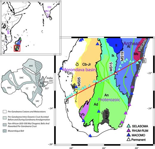
Simplified geological map of southern Madagascar (after Boger et al. 2008, 2009a, b; Tucker et al. 2011, 2014) and distribution of the seismic stations (triangles) used in this work. All indicated stations were used for the dispersion analysis, while only stations close to the red line were used for the S receiver function study. Locations of major shear zones (green lines) after Martelat et al. (2000). Thick black line delimits the boundary between the Phanerozoic–Cenozoic sedimentary basins and the Proterozoic–Archean basement domains. Insets show larger scale context of the study region and Gondwana reconstruction after amalgamation at the end of the Neoproterozoic/Cambrian (modified after Boger et al. 2019). Main map: Cn: Cenozoic sediments, Cr: Cretaceous sediments, Cb-Jr: Carboniferous-Jurassic sediments, Vl:volcanis, Ad-Vl: Volcan de l’ Androy; Tectonic domains Vb: Vohibory, Ad: Androyen, An: Anosyen, Ik: Ikalamavony, It: Itremo, At: Antananarivo, Ms: Masoara. Insets: M: Madagascar; ANS: Arabian-Nubian Shield; CC: Congo Craton; L: LATEA Terrane; SAC: South African Craton; SGT: Souhtern Granulite Terrane; SMC: Sahara Meta-Craton; TC: Tanzania Craton; WAC: West African Craton; SGT: Southern Granulite Terrian, WDC: Western Dharwar Craton, EDC: Eastern Dharwar Craton.
For a long time, the knowledge of the lithospheric thickness beneath Madagascar was based only on continent-scale or global surface wave tomographic models (e.g. Pasyanos & Nyblade 2007; Priestley et al. 2008; Fishwick 2010; McKenzie et al. 2015). These studies suggested that the thickness of the lithosphere in Madagascar is ∼90–120 km, much thinner than in the regions of East Africa (between 150 and 200 km, e.g. Pasyanos & Nyblade 2007; Priestley et al. 2008; Fishwick 2010; McKenzie et al. 2015), which were immediately adjacent to Madagascar in Gondwanaland. However, these large-scale studies used only a single station in Madagascar (ABPO in central Madagascar) so the resolution in Madagascar was very limited. Several seismological studies of the deep structure of Madagascar have been conducted recently. By joint inversion of receiver functions beneath four permanent stations and Rayleigh surface wave dispersion extracted from the Pasyanos & Nyblade (2007) map, Rindraharisaona et al. (2013) found hints for the presence of asthenospheric upwelling beneath central Madagascar. This observation was confirmed by the higher resolution shear wave models of Pratt et al. (2017), which they derived from Rayleigh phase velocities across the temporary MACOMO array (Wysession et al. 2012). Their results reveal the presence of low upper mantle S-velocity zone beneath several regions that were affected by the Cretaceous and Quaternary volcanic activities. Ramirez et al. (2018) observed a roughly circular pattern in central Madagascar and attributed this to upwelling asthenosphere, maybe triggered by lithospheric delamination. In other parts of Madagascar they interpret the ENE–WSW fast directions to the large-scale regional mantle flow field. Reiss et al. (2016) analysed teleseismic shear wave splitting in southern Madagascar and observed splitting with a NW–SE fast direction within a ∼200-km-wide zone, mostly beneath the Proterozoic tectonic domains, which they interpreted as fossil lithospheric anisotropy formed by large-scale shearing during the continental collision. Rajaonarison et al. (2020) modelled the mantle flow beneath Madagascar and offered an alternative interpretation of the splitting measurements; they suggested that the horizontal anisotropy in Madagascar originates mostly from the asthenosphere and is dominated by edge-driven convection (EDC).
Dreiling et al. (2018) observed upper-to-middle crustal radial anisotropy in southern Madagascar within the Precambrian domains and also attributed this anisotropy to past deformation related to the Pan-African orogeny. Using joint inversion of receiver functions and ambient-noise derived Rayleigh wave dispersion, Rindraharisaona et al. (2017) found that the Archean crust in southern Madagascar is thicker than the Proterozoic crust due to a fast lowermost crustal layer only present in the Archean crust. Crustal thickness decreases toward the coasts with the thinnest crust beneath the Morondava Basin, which completely lacks a lower crustal layer. Andriampenomanana et al. (2017) also used joint inversion of receiver functions and Rayleigh phase velocities, but across a sparser array covering entire Madagascar. They observed the thickest crust in Madagascar broadly below the topographic high in its central part north of 20°S, to the north of our study area. Previous studies from gravimetric data (Fourno & Roussel 1994; Rakotondraompiana et al. 1999) share the conclusion that the crust in the central part is thicker than the one along the coasts.
3 S-WAVE RECEIVER FUNCTION
3.1 Data and methods
For the S-wave receiver function analysis, only stations along the main profile were utilized (Fig. 1). This includes 25 broad-band stations from the temporary deployment SELASOMA (FDSN network code ZE, operated 2012–2014, Tilmann et al. 2012) as well as MACOMO (XV, operated 2011–2013, Wysession et al. 2012) station LONA and the permanent station VOI (GE, operated since 2009, GEOFON Data Centre 1983). For VOI station, we only used data between 2011 and 2014 (during the operational time of the temporary stations). Events at epicentral distances between 55° and 85° and with magnitudes >5.6 were considered (Fig. S1) for the receiver function computation. After visual inspection, a total of 321 waveforms from 72 events (Fig. S1) were selected for further analysis.
To compute the S-wave receiver function, all records were bandpass filtered between 1 and 30 s. We first windowed the data between 300 s before and after the S-onset and rotated the data into LQT components using the backazimuth and the theoretical incidence angle (Kind et al. 2002). Then the Q-component was deconvolved from the L-component using water level deconvolution. In the S-wave receiver function, the S to P converted waves arrive before the direct S wave. So in order to make them similar to equivalent P-wave receiver functions, the time and amplitude axes of the L component were inverted. The resulting receiver functions were inspected once again, resulting in a final data set of 306 receiver functions for further analysis. We stacked the remaining receiver functions to produce a Common Conversion Point (CCP) stack image (Yuan et al. 2000; Kind et al. 2002). We used the average shear wave model for the Precambrian domains derived from the surface waves and ambient noise dispersion (see Section 4) for time-to-depth conversion. Before computing the average, the P-wave velocities models (VP) were computed using the VP/VS ratio from Rindraharisaona et al. (2017) for the crust. For the lithopsheric mantle, the VP/VS was set to be 1.79 between the crust until 170 km and 1.81 below this depth, same as the IASP91 model (Kennett & Engdahl 1991). Conversions below the sedimentary basin will appear to be shallower by approximately ∼4 km at 150 km depth due to the differences in the structure below the sedimentary basin in the west and the Precambrian domains.
3.2 Results
S receiver function stacks for each station are shown in Fig. 2. The positive phase at 2.9−3.4 s for stations located in the Morondava basin and 3.4−5.0 s for stations in the Precambrian formations is the Moho S-to-P conversion. The negative phase between 11.5 and 13.4 s beneath the sedimentary basin and between 13.1 and 15.0 s under the Precambrian basement is interpreted as the LAB, in accordance with the surface wave derived LAB (see next sections). The CCP stack along profile AB is presented in Fig. 3. The positive Moho and negative LAB phases can be identified throughout the profile and are marked by green and red dashed lines in Fig. 3, respectively. The Moho is interpolated between neighbouring stations, where the image is ambiguous (e.g. between stations MS08 and MS09). To assess the reliability of our obtained S-wave receiver function, we compare the obtained Moho with the P-receiver function results of Rindraharisaona et al. (2017). Although the Sp converted wave is not as clear as the Ps, the resulting depths from the two methods are comparable (Fig. 3). Both the Ps and Sp receiver conversions show that the crustal thickness increases eastward with the thickest crust beneath the Archean basement.
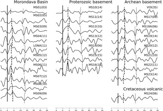
Stacked receiver functions at each station, computed using a low-pass filter of 1 s. Pms phases in receiver functions were moved out corrected using a reference slowness of 0.056 km s–1 before the summation. Station code and the number of receiver functions are shown above each trace. For each plot, the solid vertical line marks the t = 0, dashed vertical lines indicate the observed Moho phase and dotted vertical lines correspond to the LAB phases.
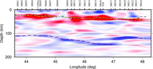
CCP stacking image for the S receiver functions along profile AB (Fig. 1). Positive and negative velocity contrasts are shown in red and blue, respectively. The green line shows the interpreted Moho based on the Sp conversions shown in the image, whereas the black dashed line indicates the Ps Moho from Rindraharisaona et al. (2017) for comparison. The dashed red line shows the strongest negative amplitude between 110 and 200 km, representing the LAB; the dotted line extends this where there are overlapping negative conversions at LAB depths.
The LAB is simply picked as the strongest negative amplitude between 110 and 200 km depth. Throughout the profile, the LAB depth varies between 110 and 146 km. Between approximately MS15 (46.3°E) and MS19 (47.2°E) two overlapping negative conversions can be identified, where simply the strongest one is chosen, leading to an apparent jump in LAB depth by some 20 km at 47°E, which is most likely not real. Along the Eastern part of our profile the tomographic model of Pratt et al. (2017) shows a strong N–S gradient in shear velocity at these depths. So we consider the double LAB to be most probably an artefact of LAB topography oblique to the profile. If this interpretation is correct, then the shallower LAB might indicate the LAB to the north of the profile and result from events with northerly backazimuths.
4 SURFACE WAVE ANALYSIS
4.1 Dispersion measurements and tomographic inversion
For the dispersion curves measurements, we primarily used the data from the 25 broad-band stations in the temporary deployment SELASOMA, supplemented by 8 temporary stations from the MACOMO project, 5 temporary stations from RHUM-RUM (YV, operated 2012–2014, Barruol et al. 2017) and the permanent stations FOMA (G, operated since 2008, IPGP 1982) and VOI in southern Madagascar (Fig. 1). From teleseismic events with Mw > 5.6 and epicentral distances >30° we selected 173 events for Rayleigh and 85 events for Love wave analysis (Fig. S1). Detailed selection criterion can be found in Section S1.
We used the two-station method for the phase velocity measurement. This method is a special case of the frequency domain slant-stack method (Park et al. 1998) for several stations. For each station-pair dispersion measurement, the event must lie approximately on the same great circle path (±5°) as the two stations. In this case, it can be assumed that the Rayleigh wave to both stations has approximately the same source radiation effect and has experienced the same structure on the way to the close station, such that the difference between the surface wave recording at the close and far stations is only influenced by the structure between them. We transferred the near station seismogram to the far station by applying phase shifts according to the difference in epicentral distances and frequency-dependent reference phase velocities based on the predicted dispersion from PREM (Dziewonski & Anderson 1981) with a modified crustal structure from Rindraharisaona et al. (2017). Love and Rayleigh waves were analysed in the same way, using the transverse and vertical components, respectively. More details on the measurement procedure and example are given in Section S1 and Fig. S2. The median of the dispersion curves derived from all events for the same station-pair was used for the tomographic inversion for the phase velocity maps. The standard deviation was computed for each station pair to represent the error of the phase velocity measurement.
To extend the dispersion curves to shorter periods, we amend our measurements with the Rayleigh and Love phases dispersion curves from ambient noise data provided by Dreiling et al. (2018), which cover the range 5–30 s. Our dispersion curves are in agreement with those from the ambient noise with differences of less than 0.05 km s–1 at most of the common periods (Fig. 4). We therefore feel confident to combine them for the joint inversions. Thus, the entire data set contains only ambient noise data at periods of <15 s, both ambient noise and earthquake data at periods of 15−25 s, and exclusively earthquake data at periods of >25 s. Before the tomographic inversion, we have converted the phase velocities into phase arrival times t such as t = d/c, where d is interstation distance and c is the phase velocity.
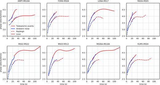
Phase velocity dispersion curves from ambient noise data (blue) (Dreiling et al. 2018) and from teleseismic events (red) for 8 sample station pairs. Solid and dashed lines denote Love and Rayleigh phase velocities, respectively. Dispersion curves from the two data sets are comparable at periods where they are overlapping, with differences mostly <0.01 km s–1.
The Fast Marching Surface wave Tomography method (FMST, Rawlinson & Sambridge 2004, 2005) was then used to invert the dispersion curves for surface wave velocity models. The model grid nodes were set to be spaced 0.5° apart in latitude and longitude. A computational grid of 0.003° was used for the forward calculations in the Eikonal tomography. We used a homogeneous starting model, which was derived from applying the slant-stack method of the stations along profile AB for periods ≤80 s and the median of all inter-station dispersion curves for longer periods (≥80 s). The trade-off between the misfit and model variance was analysed for damping factors between 0 and 400. An example of tradeoff curves is plotted in Fig. S4. Where a minimum exists for a given trade-off curve we chose that point as the preferred damping value, otherwise we chose a point where further increases in model variance only resulted in minor reductions of the data variance.
4.2 Phase velocity tomography
Figs S5 and S6 show the path coverage for 20, 30, 40, 60, 80 and 100 s for Rayleigh and Love waves, respectively. The path coverage is good for periods of 20−80 s, but exhibits more gaps for longer periods (>80 s). The path coverage from the earthquake records is very limited at shorter periods (<20 s), but by adding the data obtained from the ambient noise correlation (Dreiling et al. 2018), as mentioned above, we obtained fairly good path coverage along the SELASOMA profile at all considered periods (5–100 s). In Fig. 5, we compare Love and Rayleigh wave phase velocities curves between the sedimentary basin and Precambrian basements. For Rayleigh waves, at smaller periods (20−60 s), the sedimentary basin is slower than the Precambrian basement, but becomes faster at longer periods (60−100 s). However, for Love waves, the sedimentary basin is faster at shorter periods (20−60 s) than the Precambrian basement, but becomes slower at longer periods (60−100 s).
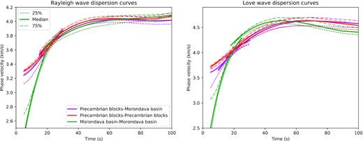
Averaged Rayleigh and Love wave dispersion curves for sub-regions of the sedimentary basin (green lines) and Precambrian basement (red lines), respectively. The dispersion curves at short period are from ambient noise data (Dreiling et al. 2018).
We conducted checkerboard tests to evaluate the resolution power of the FMST tomography (Section S2). Wave speed variations occurring over a distance of larger than ∼100 km (checker board grid size 1° × 1°) can be well recovered for periods up to 60 s along the profile and in most of the study areas, for both Rayleigh and Loves waves, and variations occurring over distances of ∼150 km can be well recovered at all periods considered, that is up to 100 s (Figs S7 and S8).
The tomographic maps for different periods are shown in Figs 6 and 7 for Rayleigh and Love waves, respectively. The resulting tomographic maps indicate that for Rayleigh wave phase velocity, at longer periods (≥60 s), the Archean basement exhibits faster velocity than the Proterozoic and the sedimentary basin (Fig. 6). For Love waves, in general, the western part is always faster than the eastern part (Fig. 7). At first sight, this observation appears to be inconsistent with Fig. 5, which shows that at longer periods the sedimentary basin exhibits a relatively slower velocity at long periods. This can be explained by the fact that the Morondava basin–Morondava basin dispersion curves in Fig. 5 are exclusively derived from the (approximately NS) paths between the MACOMO station close to the west coast right at the northern edge of our study area and a few stations along the profile (Fig. S6). However, EW paths (i.e. Precambrian blocks-Morondava basin, Fig. 5) dominate the tomographic model along the SELASOMA profile, and both sets cover different areas. We note that because of the uneven ray coverage, the tomographics maps are only considered reliable along the main profile. The maximum error of our map are 0.06 and 0.05 km s –1, at different periods, for Rayleigh and Love waves, respectively (Figs S9 and S10). These errors were estimated from the bootstrap samples and are unreliable in the regions with poor ray path coverage (see Section S3 for more information). In Fig. S11, we compare our Rayleigh wave velocity maps with those derived from Pratt et al. (2017). Some differences between the two results are observed along the main profile, particularly at longer periods, presumably because of our higher station density, while they are consistent within 0.1 km s–1 elsewhere.
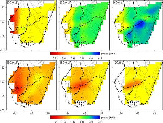
Rayleigh wave phase velocity maps. Bold black line indicates the boundary between the sedimentary basin and the Precambrian domain. Thin black lines divide the different geological blocks. In general, the eastern part of Madagascar is faster than the western part. At longer period, the number of the path between Morondava basin–Morondava basin is very limited and only between station along the main profile and stations in the north (Fig. S5), thus the inconsistent between the observed tomographic maps and the dispersion curves in Fig. 5.

Same as Fig. 6 but for Love waves. At longer period >60 s, in contrast to the Rayleigh wave, the eastern part of Madagascar is slower than the western part. Same as Fig. 6, the disagreement between the tomographic maps here and the dispersion curves in Fig. 5 is due to the limited number of dispersion curves between Morondava basin–Morondava basin along the main profile Fig. S6.
4.3 Shear wave velocity and radial anisotropy inversion
The resulting phase velocities beneath profile AB (Fig. 1) were extracted from the tomography results (Figs 6, 7) and then inverted to obtain the 1-D shear wave velocity structure, using the surf96 routine of Herrmann (2013). To help constrain the crustal S-wave velocity, we also included the Rayleigh and Love wave group velocities from previous works (Dreiling et al. 2018; Rindraharisaona et al. 2017). The starting model was constructed from Rindraharisaona et al. (2017) for the crust and either PREM (Dziewonski & Anderson 1981) or AK135 (Kennett et al. 1995) for the mantle. The velocity structure was parametrized with layers of 1 and 2 km thickness for the top two layers, then 2.5 km between 3 and 60.5 km, and 5 km between 60.5 and 250 km.
To estimate the error of the extracted dispersion curve from the tomography model, we used the bootstrapping method. For each inversion, we constructed a bootstrap sample with the same number of earthquakes as in the actual data set. The contributing earthquakes were chosen from all available with replacement, i.e. each earthquake could be picked more than once, or not at all. We computed the median and standard deviation for each station pair. Then, we performed the tomography inversion using the same damping factor, for each inversion. After that, we extracted the shear wave velocity beneath each station. This process was repeated 100 times. We computed the standard deviation for each period and used it as the error in the dispersion curves. More details about the bootstrapping method are given in Section S3.
Both the Love and Rayleigh wave dispersion curves were simultaneously inverted for an isotropic model at the beginning. However, it was impossible to fit the two data-sets with an isotropic model. Therefore we separately inverted the Love and Rayleigh waves dispersion curves, effectively attributing the difference between VSH and VSV to the presence of radial anisotropy.
The separate inversion approach has been used extensively in prior studies (e.g. Becker et al. 2008; Fu et al. 2018), although some other studies (e.g. Lebedev et al. 2009) have simultaneously inverted VSH and VSV. When computing the radial anisotropy (RA) from the VSH and VSV, the question arises whether apparent RA can arise as an artefact of the data distribution, for example the ray path distributions or errors in the dispersion curves. To check the plausibility of this possibility we (i) compared the preferred model to a model based on a 2-D inversion, where the number of Rayleigh paths has been reduced to match the coverage of the Love wave, (ii) inverted the Love dispersion curve, using the SV model as starting point, and vice versa inverted the Rayleigh dispersion using the SH model as starting point and (iii) considered the variation of RA based on bootstrap resampling of earthquake dispersion records. All procedures result in a similar RA dependence with depth (see Section S3 for details).
Fig. S12 shows for reference a model constructed from the averaged dispersion curves in Madagascar but because of lateral heterogeneity it should not be interpreted directly. An example of the tests carried out to assess the uniqueness and reliability of the resulting model is shown in Fig. S13 for a location coincident with station MS15 in the central part of the profile (Fig. 1).
The RMS of the misfit between the observed and predicted phase velocities are generally good (less than 0.12 km s–1 for Rayleigh and 0.15 km s–1 for Love wave) within the study areas, for the different periods (Figs S14 and S15). For a depth shallower than 200 km, the bootstrapping and starting model tests indicate a maximum error of 0.05 km s–1 for the shear velocity models ( VSV and VSH, Fig. S18).
4.4 Results
Fig. 8 shows the isotropic model of the shear wave velocity and RA along the SELASOMA profile (see Fig. 1 for location); a comparison of the absolute values of VSV and perturbations of VSV and VSH relative to PREM is shown in Fig. S19. We only discuss the mantle structure because the crustal structure was already discussed in detail by Dreiling et al. (2018) and Rindraharisaona et al. (2017).
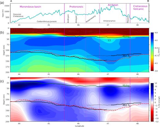
Cross-sections along profile AB. (a) Elevation. (b) Absolute isotropic velocity |$V_{\rm iso}=\sqrt{\frac{2}{3}V_{\rm SV}^2+\frac{1}{3}V_{\rm SH}^2}$|. (c) Radial anisotropy. Green and black lines mark the Moho and the LAB, respectively, derived from receiver functions data. Dotted lines mark a secondary negative arrival of nearly similar strength identifiable in the S receiver functions (see Fig. 3). Red line indicates the LAB estimated from the strongest negative velocity gradient between 50 and 200 km. Continuous, dashed and dotted vertical lines separate the different geological domains.
Several techniques have been used to estimate the depth of the LAB (e.g. Simons & Van Der Hilst 2002; Weeraratne et al. 2003; Debayle et al. 2005; Priestley & McKenzie 2006; Eaton et al. 2009). Each method has its advantages and limitations. In our case, we interpret the high velocities to represent the lithospheric mantle and, as recommended by Weeraratne et al. (2003), use the definition that the depth to the strongest negative velocity gradient corresponds to the LAB . The estimated LAB depth from the isotropic shear wave velocity structure using this definition (red line in Fig. 8) is in a excellent agreement with that derived from the S-RF method (black line) over most of the study area. East of 47° the comparison is hindered by the apparent double conversion. If we take the deeper conversion as the real LAB, then the agreement is also good in the central part (see Section 3.2 for the justification why this is a reasonable assumption to make). The LAB depth increases gradually from the west (∼110 km) to the western part of the Archean domain (∼150 km), and then decreases to ∼120 km beneath the volcanic formation.
The observed discrepancy between the VSV and VSH models (Fig. S19) indicates the presence of strong RA (Fig. 8c). As discussed in Section S3, the error in our RA is less than 1 percentage point at depths shallower than 200 km. The western Morondava basin below the Cenozoic–Cretaceous sediments appears to have the highest discrepancy between the VSV and VSH models and thus RA within the lithosphere has a maximum value of 9 per cent. The Proterozoic domains show small (1–5 per cent) to vanishing positive RA, while a stronger RA is observed beneath the Archean crust (maximum value 6 per cent). Below the lithosphere at a depth of about 150 km a negative RA is observed. A negative RA also appears at the westernmost edge of the profile, but is not well resolved. In contrast, a positive RA in the asthenosphere is observed in the middle of the profile, beneath the Carboniferous–Jurassic sediments of the eastern Morondava basin and the Proterozoic basement.
5 DISCUSSION
The estimated depth of LAB confirms previous observations of a relatively thin lithosphere compared to the formerly adjacent area of East Africa. Compared to the regional African surface wave tomography models (e.g. Pasyanos & Nyblade 2007; Priestley et al. 2008; Fishwick 2010; McKenzie et al. 2015), our lithospheric thickness is similar to these larger scale studies beneath the Morondava basin (∼110 km), but is 10–70 km thicker beneath the Precambrian basement (Fig. S19), where prior studies had inferred an extremely thin lithosphere. Although all studies differed in the exact method to extract the thickness of the lithosphere, the difference can probably largely be attributed to lack of resolution in those prior studies due to paucity of data from Madagascar. In this context we also note that the surface wave tomography model of Pratt et al. (2017) shows considerable north-south variation in upper mantle structure, and the IRIS GSN station ABPO used in all of the continental-scale tomography is placed above relatively slow uppermost mantle.
Anisotropy in the mantle is typically interpreted as crystal preferred orientation of anisotropic minerals (CPO; e.g. olivine). Ductile flow very often leads to the development of CPO, in these cases RA can directly depict shear strain under conditions prevalent in the lower crust and mantle. Positive RA is associated with near horizontal fabrics such as horizontal layering, compositional banding or horizontal shear fabrics, while negative RA implies the existence of near vertical features that may include deformation structures such as faults, fault-, shear-, fracture zones or magmatic dikes. Considering the complex geology of Madagascar and the pattern of the resulting shear wave velocity (Figs 8 and S19), the observed RA cannot be associated with a single process in the south of Madagascar. Our resulting models show that the shear wave velocity structure changes at short distances reflecting the different geological settings.
In the following, we will discuss the observed velocity structures, lithosphere thickness and the RA for the different geological units in southern Madagascar. We will only focus on the lowermost crust and the lithospheric mantle in our discussion, as the crustal velocity structure and RA in the upper-middle crust (∼ 30 km) have been previously discussed (e.g. Dreiling et al. 2018; Rindraharisaona et al. 2017). For convenience, we will also discuss the asthenospheric structure in the context of these geological domains, even though they are unlikely to directly shape it. Although asthenospheric depths are less well resolved than the lithosphere, some first order variations are still indicated to be resolvable by our tests (in particular Figs S13 and S18).
5.1 Sedimentary Morondava basin
The results beneath the Morondava Basin suggest that the lithospheric mantle has been significantly modified after its formation. The lithospheric mantle beneath the Morondava Basin is thinner compared to those beneath the Precambrian basement (Figs 3, 8 and S19). If we assume that the fast velocities at depths down to 110 km represent the inherited fast velocity from the Proterozoic lithosphere underlying the Morondava Basin and that it had a comparable thickness before the breakup of Gondwana, the thinning of the lithosphere would be associated with the formation of the sedimentary basins during the Mesozoic Karoo failed rifting, Jurassic rifting and break-up between Madagascar–India and Africa. The mantle lithosphere beneath the Morondava basin has been thinned more strongly than the crust (Fig. 9), which can be an indication of the depth-dependent thinning as it has been seen in many continental margins (e.g. Kusznir & Karner 2007, and references therein).
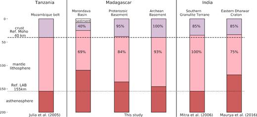
Lithosphere thicknesses in Tanzania, Madagascar and India. Note that crustal thickness for the Eastern Dharwar Craton is from Julià et al. (2009), obtained from the joint inversion of receiver function and surface wave dispersion curves. Crustal thickness for Madagascar is from Rindraharisaona et al. (2017), which they used the joint inversion of receiver function and surface wave dispersion curve to estimate the crustal thickness. In this figure the crustal thickness and the LAB for the Mozambique belt in Tanzania is assumed as reference. The remaining percentage shown here is the ratio between the deformed and referenced crustal thickness for crust and referenced total lithospheric thickness for the lithosphere (fl, fc in Sandiford & Powell 1990).
At a depth of 25−50 km in the mantle lithosphere beneath the sedimentary basin, negative VSV and positive VSH anomalies (with respect to PREM) are observed (Figs S19c and d), resulting in a large positive RA of up to 9 per cent. The pronounced positive RA may be caused by the sub-horizontal alignment of anisotropic minerals, which was acquired during the crustal-lithospheric thinning related to extension during development of the Morondava Basin. The deeper part of the mantle lithosphere (50–100 km depth) is instead characterized by relatively weak (positive) anisotropy. One can speculate whether the boundary between the two regimes represents the boundary between the original stretched lithosphere (shallow part) and the regrowth by post-rift thermal equilibration.
A positive RA (up to 5 per cent) is observed beneath most of the basin; the small region of negative RA west of 44°E is at the edge of our model and not well resolved, so we do not interpret it. The few available estimates of shear wave splitting at SELASOMA stations in the basin indicated fast directions parallel to the ENE–WSW absolute plate motion, or in the case of null splitting measurement, are at least consistent with this fast direction (Reiss et al. 2016). Therefore, the dominant horizontal fabric in the asthenosphere is maybe most easily explained by a shearing layer between the moving lithosphere and the deeper mantle (Couette flow). However, the MACOMO station LONA close to the profile indicated a N–S fast directions (Ramirez et al. 2018), showing small-scale variability.
5.2 Proterozoic basement domains
Both the velocity structure from the isotropic wave model and the LAB from the S-wave receiver function show that the lithosphere thickness beneath the Proterozoic basement of the Androyen, Anosyen and Ikalamavony domains is ∼125–145 km (Fig. 8). The lithospheric mantle is characterized by an average positive velocity anomaly of ∼3 and ∼5 per cent relative to PREM for VSV and VSH, respectively (Figs S19c and d). Thus, a moderately positive RA of 1−5 per cent is observed beneath the area, which indicates the presence of horizontally oriented fabric. This fabric is most-likely associated with fossil anisotropy in the lithosphere. The Pan-African orogeny and associated final amalgamation of Gondwana had a major imprint on southern Madagascar that experienced deformation, magmatic and metamorphic events (e.g. Martelat et al. 2000; Giese et al. 2011; Tucker et al. 2011; Martelat et al. 2014; Tucker et al. 2014, and references therein). Reiss et al. (2016) also have associated the azimuthal anisotropy beneath the Proterozoic domains to a fossilized anisotropy due to ductile deformation during the Pan-African orogeny.
The lithosphere here is thinner than stable Proterozoic regions elsewhere (e.g. Artemieva & Mooney 2001). Southern Madagascar was affected by the Pan-African orogeny (e.g. Dissanayake & Chandrajith 1999), which had modified at least the crustal structure (e.g. Rindraharisaona et al. 2017; Dreiling et al. 2018). We compare the lithospheric structure in southern Madagascar to East Africa, which is also part of the Pan African Mozambique belt. In general, the lithospheric thickness beneath the areas that formed part of the Pan-African orogen is thin (90–160 km), compared to those beneath the Proterozoic–Archean basement elsewhere (160–250 km, e.g. Artemieva & Mooney 2001; McKenzie et al. 2015). The lithosphere thickness (∼125–145 km) we obtained beneath the Proterozoic crust is 10–30 km thicker than previously reported on the basis of continental scale tomography for Madagascar (e.g. Pasyanos & Nyblade 2007; Priestley et al. 2008; Fishwick 2010; McKenzie et al. 2015), but its average is still substantially thinner than what has been reported for the Mozambique belt in Tanzania (∼155 km, e.g. Julià et al. 2005; Priestley et al. 2008; Fishwick 2010). However, the observed upper mantle lid velocities of 4.5–4.7 km s–1 (VSV) are similar to previous results. It is possible that the Proterozoic lithosphere in Madagascar was similar in thickness to that in East Africa but thinned during extension associated with the separation of Madagascar–India and Africa. The thinning of the lithosphere could be associated to a depth-dependent lithosphere stretching, which is also in agreement with the positive radial anisotropy observed there.
5.3 Archean basement
Relative to PREM, a negative VSV (−3 per cent, at the the uppermost mantle) and a positive VSH (+4 per cent) anomalies are observed beneath the Archean basement (Figs S19c and d), indicating a strong positive RA of max +6 per cent (Fig. 8c). We assume that the large positive RA beneath the Archean basement is due to the CPO and was likely increased during the lithospheric extension in the Cretaceous when India rifted away from Madagascar. The source of the azimuthal anisotropy in the lithospheric mantle was also attributed to a fossil anisotropy by Reiss et al. (2016). Compared to the typical craton elevations worldwide (except for South African and Tanzanian cratons, Artemieva & Vinnik 2016, table 1), the topography of the Antananarivo domain appears to be relatively high (Fig. 8a). The crustal thickness is also larger in the Antananarivo block than in the average Archean domains elsewhere due to the presence of an underplate layer (Rindraharisaona et al. 2017). However, the low-velocity (and presumably low density) anomaly at the top the mantle lithosphere (L1 in Figs 8b, S19b and c) might also contribute.
Alternatively, the high topography in the Antananarivo domain may also indicate the presence of hot and buoyant mantle upwelling beneath the Archean lithosphere, which could be associated with a thermal anomaly that had produced the recent uplift in the Antananarivo Domain (Roberts et al. 2012). It could be associated with the lithospheric delamination, which has been hypothesized in previous studies (e.g. Pratt et al. 2017; Ramirez et al. 2018); the upwelling return flow is one possibility for explaining the negative anisotropy observed in the asthenospheric mantle beneath the Archean lithosphere. Although the structure of the asthenospheric mantle is at the margin of resolution, our test suggests it can be resolved with maximum RA error of 1 per cent between 120 and 200 km depths (Fig. S18, MS19 in Fig. 1).
Another plausible explanation of the negative RA observed in the asthenospheric mantle beneath the Antananarivo domain and the volcanic formation along the eastern coast is the presence of the asthenospheric downwelling related to the Réunion mantle plume (Mazzullo et al. 2017). In fact, Figs 8 and S19 indicate that the asthenospheric velocities in the eastern part (i.e. beneath the Antananarivo domain and volcanic formation) are lower than those in the western part. This observation does not favor the presence of astenospheric upwelling. Mazzullo et al.’s (2017) anisotropic tomography of the Rayleigh wave around the La Réunion island suggests the presence of a large low velocity zone (∼6 per cent) beneath the Réunion island, which extends to the east coast of Madagascar (fig. 10 cross section DD’ in Mazzullo et al. 2017). Furthermore, Storey et al. (1995, 1997) suggest that mantle plumes may have played an important role in flood basalt formations, along the eastern coast. Thus, the presence of the asthenospheric downwelling is also possible or even likely, at least beneath the volcanic formation.
5.4 Gondwanan context
As we mentioned in Section 2, during the Gondwanaland assembly the Madagascan basement was located between India and Africa (Fig. 1). The position of the Antananarivo Domain before/during the Gondwana assembly has been debated. Some authors suggested it has collided with the Indian Dharwar Craton in late Archean times and shared a common evolution as the greater Dharwar Craton thereafter (e.g. Tucker et al. 2011, 2014). However, others interpreted it as individual terrane called ‘Azania’ with African affinities that collided with the Indian Dharwar Craton after Ediacaran times (∼600 Ma, near the end of the Proterozoic, e.g. Collins 2000; Collins & Pisarevsky 2005). Fig. 9 compares the lithospheric structure in the Antananarivo Domain to that of the Mozambique Belt, Tanzania Craton and India. From S-wave tomography and estimating the LAB from a reduction of VSV >1.25 per cent , Maurya et al. (2016) found a lithosphere thickness of ∼120 km in the Eastern Dharwar Craton, which is ∼5–30 km thinner than the lithosphere thickness beneath the Antananarivo Domain (∼ 125–150 km). Mitra et al. (2006) estimated the lithosphere thickness to be ∼155 km in the region affected by the Pan African Orogeny in southern India (Southern Granulite Terrane) based on the Rayleigh wave phase velocity dispersion. From joint inversion of receiver function and Rayleigh wave dispersion curve, the LAB was observed to be at depth of ∼150 km beneath the Mozambique Belt (Julià et al. 2005). The lithosphere thickness beneath the Antananarivo domain is comparable to the lithosphere to those beneath the Southern Granulite Terrane and Mozambique belt in Tanzania.
6 CONCLUSIONS
We computed S-wave receiver functions and applied the two-station method to measure Rayleigh and Love waves dispersion curves between 15 and 100 s. We obtained 3-D shear waves velocities and radial anisotropy. The LAB from the two methods are in agreement within 5 km and show a lithospheric thickness ranging from 110 km in the western part of southern Madagascar, below the Morondava basin to 150 km below the western part of the Archean Antananarivo domain and it then decreases toward the east coast, with a depth of ∼120 km beneath the volcanic formation. The estimated LAB is deeper than previous continental scale surface wave tomographic studies suggested, but thinner than in the Mozambique belt in Tanzania. Positive RA up to 9 per cent is prevalent in the shallower part of the mantle lithosphere. Positive RA is observed in the lithospheric mantle in southern Madagascar, especially at depths less than 75 km, and with varying strengths below the different parts of Madagascar. The positive RA probably represents the near-horizontal orientation of the fabric, most likely formed by lithospheric extension during failed-rifting, rifting and break-up from Africa (Morondava Basin) and/or India (Archean basement). The modification of the mantle lithosphere beneath the Proterozoic basement most likely occurred during the Pan-African orogeny, which resulted in the positive RA observed in there. Although the resolution is weaker in the asthenosphere, there seems to be an identifiable pattern of positive RA below the eastern part of the Morondava basin and the Proterozoic domains, and a negative RA below the eastern-most part of Madagascar, including the Antananarivo block and the Cretaceous Volcanics. This negative RA suggest the presence of mantle upwelling there and may explain the high topography in the high plateau. The presence of mantle downwelling due the mantle plume activity cannot be ruled out here.
SUPPORTING INFORMATION
Figure S1 Left-hand panel: earthquake distribution used for the S-wave receiver function computation. Right-hand panel: distribution of the teleseismic events used to compute the Love and Rayleigh phases dispersion curves. Yellow circles indicate events used for the Rayleigh wave analysis only, cyan circles mark the events used for Love wave analysis only and pink circles show the events used in both Rayleigh and Love waves analysis.
Figure S2 Example of the phase velocity measurements for the station pair MS05 and MS22. (a) Original seismogram for MS05 and transferred seismograph for MS21 with the transfer function constructed based on the modified PREM as starting model; (b) Frequency domain slant-stacking amplitude slant-stack: f−δk spectrum. The black line shows the value and range of the δk measurement. Panel (c) as (a) but the transfer function has been updated to match the refined phase velocity estimate implied by (b).
Figure S3 Number of station-pairs for which measurements could be obtained, as a function of period. This is the number of measurements from the earthquake data only. Red colors shows the number of dispersion curves for Rayleigh wave, continuous line (total), dashed line (Precambrian) and dotted line(sediment). Blue colors correspond to the number of dispersion curves for Love waves.
Figure S4 Trade-off curves between the residual phase arrival times and variance model perturbation at 30, 50, 70 and 100 s. Damping factors between 0 and 400 were used. The black point on each curve corresponds to the preferred damping factor used in the tomography inversion.
Figure S5 Rayleigh wave path coverage for different periods. The paths are colored according to the measured phase velocity between two stations.
Figure S6 Same as Fig. S5 but for Love waves.
Figure S7 Synthetic checkerboard test for the resolution of Rayleigh wave tomography with 0.5°× 0.5° grid cell with (a) 1×1, (b) 2×2, (c) 3×3, (d) 4×4 cell block size. For each line, the first column shows the input model and the columns 2–7 the recovered structures for different periods.
Figure S8 Same as S7 but for Love wave
Figure S9 Phase velocity standard error for the Rayleigh wave tomography. The error reported here is the standard deviation of the bootstrapping sample. Therefore, along the main profile, where the rays paths are denser, the error is relatively larger (see supplementary text for details). Note that the error at each node is not directly influenced by the neighbouring nodes.
Figure S10 Phase velocity standard error for the Love wave tomography. The error reported here is the standard deviation of the bootstrapping sample.
Figure S11 Comparison between our Rayleigh phase velocity maps (top) and results from Pratt et al. (2017). Differences are observed along the main profile, which is sampled much more densely in our results, and at a period of 20 s, where we observe significantly lower velocities. The Pratt et al. (2017) model covers the whole of Madagascar but for ease of comparison we have masked the Pratt et al. (2017) model according to our phase coverage.
Figure S12 (a) Average dispersion curves for Rayleigh (red) and Love (blue) waves. The dispersion at each grid point between 44°E and 48°E and between 24.0°S and 21°S were averaged. Dashed and continuous lines indicate the observed and inverted dispersion curves, respectively. For each period, the errors plotted here are the average of the error discussed in Section S3. (b) Absolute isotropic velocity (green, lower scale) and RA (magenta, upper scale) obtained from inverting the average dispersion curve in Fig. S12(a).
Figure S13 Examples of testing the reliability of the obtained velocity structure and RA for the grid location of station MS15. (a) Bootstrap test. The top plot shows the inverted Rayleigh (boot_R) and Love (boot_L) dispersion curve from the bootstrapping sample. The standard deviation from the observed bootstraping sample are plotted together with the observed dispersion curve used in Fig. 8, in magenta (Rayleigh, obs_R) and cyan (Love, obs_L). The inverted dispersion curves corresponding to the shear wave velocity model in Fig. 8 are plotted in red (Rayleigh) and blue (Love) dashed lines. The bottom figure shows the velocity models for all bootstrap samples. (b) Inversions of the Rayleigh wave dispersion curve with different starting models. In each model a low velocity zone was placed at different depths of 75, 100, 125, 150 and 200 km in the starting model. (c) Inversions using different starting models: AK135 (dashed line), PREM (solid line) and 5 per cent slower (dash–dotted line, i.e. PREM -5 per cent) and faster (dotted line, i.e. PREM +5 per cent) then PREM. Different starting models resulted in a comparable final model (only the final models are plotted for clarity, except PREM). (d) Final models inverted using the Rayleigh (red) and Love (blue) waves dispersion curves. The dashed lines with error bars and solid lines are the observed and synthetic dispersion curves, respectively. The red dotted line is the synthetic Love wave dispersion curve predicted by the final VSV model (i.e. assumed VSV = VSH); the blue dotted line is the synthetic Rayleigh wave dispersion curve predicted by the final VSH model. The difference between the observed and predicted dispersion curves indicates the presence of anisotropy.
Figure S14 Rayleigh wave maps of RMS shear velocity between observed and predicted dispersion at different periods. Note that the RMS at each node is not directly influenced by the neighbouring nodes.
Figure S15 Same as S14 but for Love wave
Figure S16 Comparison between the isotropic shear wave velocity (continuous lines, lower scale) and RA (dashed lines, upper scale) using the same ray paths (Viso same and RA same) and different number of dispersion curve (Viso same and RA different) for Rayleigh (red) and Love (blue) waves, at different location.
Figure S17 Comparison between the isotropic shear wave velocity (continuous lines, lower scale) and RA (dashed lines, upper scale) for the Rayleigh to Love and Love to Rayleigh inversion results.
Figure S18 Dispersion curves (a), radial anisotropy distribution (b) and Viso distribution (c) computed from the bootstrap samples at the grid locations of MS05, MS15, MS19. Continuous black line indicates the median off all model with the standard deviation error at each depth. The dispersion curves plotted here are the same as in Fig S13a
Figure S19 Cross-sections along profile AB. (a) Elevation. (b) Absolute SV-wave velocity structure. (c) SV-wave velocity perturbation relative to the VSV PREM. (d) SH-wave velocity perturbation relative to VSH PREM. (e) Viso relative to the isotropic velocity model PREM. Green and black lines mark the Moho and the LAB, respectively, derived from S receiver functions. The red line indicates the strongest negative vertical velocity gradient as a proxy for the LAB; the black dashed line shows the LAB estimated in the surface wave tomography of Fishwick (2010). Continuous, dashed and dotted vertical lines separate the different geological domains.
Please note: Oxford University Press is not responsible for the content or functionality of any supporting materials supplied by the authors. Any queries (other than missing material) should be directed to the corresponding author for the paper.
ACKNOWLEDGEMENTS
We acknowledge the Geophysical Instrument Pool Potsdam (GIPP) for supplying the instruments for the SELASOMA project and GeoForschungsZentrum (GFZ) for supporting the field experiment. We are very grateful to all fieldwork participants from Institute and Observatory of Geophysics Antananarivo, GFZ and University of Frankfurt. The SELASOMA data are archived and at the GEOFON data center (http://geofon.gfz-potsdam.de). We thank Guilhem Barruol (IPGP) and Michael Wysession for providing early access to the RHUM-RUM and MACOMO data sets, respectively. The RHUM-RUM and MACOMO data are available at the French RESIF data centre (http://seismology.resif.fr) and the IRIS DMC (http://www.iris.edu), respectively. Elisa Rindraharisaona was supported by the Alexander-von-Humboldt foundation with a Georg-Forster postdoctoral research fellowship. Last but not least, we thank the reviewers, the Associate Editor and Huajian Yao for constructive comments and suggestions.
