


SUMMARY
2-D full-waveform inversion (FWI) of shallow-seismic wavefields has recently become a novel way to reconstruct S-wave velocity models of the shallow subsurface with high vertical and lateral resolution. In most applications, seismic wave attenuation is ignored or considered as a passive modelling parameter only. In this study, we explore the feasibility and performance of multiparameter viscoelastic 2-D FWI in which seismic velocities and attenuation of P and S waves, respectively, and mass density are inverted simultaneously. Synthetic reconstruction experiments reveal that multiple crosstalks between all viscoelastic material parameters may occur. The reconstruction of S-wave velocity is always robust and of high quality. The parameters P-wave velocity and density exhibit weaker sensitivity and can be reconstructed more reliably by multiparameter viscoelastic FWI. Anomalies in S-wave attenuation can be recovered but with limited resolution. In a field-data application, a small-scale refilled trench is nicely delineated as a low P- and S-wave velocity anomaly. The reconstruction of P-wave velocity is improved by the simultaneous inversion of attenuation. The reconstructed S-wave attenuation reveals higher attenuation in the shallow weathering zone and weaker attenuation below. The variations in the reconstructed P- and S-wave velocity models are consistent with the reflectivity observed in a ground penetrating radar (GPR) profile.
1 INTRODUCTION
Most of the current surface wave methods are based on the extraction and inversion of surface wave dispersion curves (Xia et al. 1999). The dispersion-based surface wave methods, however, fail when strong lateral heterogeneity exists, which is regarded as one of their limitations (Pan et al. 2019). Different approaches are proposed to account for lateral heterogeneity, such as laterally constrained inversion (Socco et al. 2009), cross-correlation analysis of multichannel data (Hayashi & Suzuki 2004; Ikeda et al. 2013), and spatial windowing (Bohlen et al. 2004; Bergamo et al. 2012). Another limitation that current surface wave methods face is the uncertainty in the correct estimation and identification of multimodal dispersion curves (Boaga et al. 2013; Gao et al. 2014, 2016). Full-waveform inversion (FWI) may overcome these limitations and can produce high-resolution multiparameter models for complex geologic structures. FWI was first introduced by Tarantola (1984) and Mora (1987) in time domain with gradient-based inversion. With the rapid development of computational power, it has become increasingly popular to use 2-D FWI of surface wave to reconstruct near-surface models. Romdhane et al. (2011) and Tran et al. (2013) demonstrated the effectiveness of 2-D frequency-domain elastic FWI in reconstructing heterogeneous near-surface model. Groos et al. (2014, 2017) and Pan et al. (2016, 2018) showed that 2-D time-domain elastic FWI could efficiently delineate shallow subsurface with high resolution. Besides, 3-D FWI of the surface wave is also becoming feasible in recent years (Irnaka et al. 2019; Mirzanejad & Tran 2019). FWI of the surface wave is highly ill-posed and might be trapped in local minima, especially for the conventional least-squares misfit. One practical way to mitigate this problem is to use an initial model built by inverting surface wave dispersion curves. Besides, an alternative objective function, such as amplitude-spectrum-based misfit (Pérez Solano et al. 2014; Masoni et al. 2016), envelope-based misfit (Wu et al. 2014; Yuan et al. 2015), and multi-objective misfit (Pan et al. 2020), can be used to reduce the nonlinearity of surface wave FWI.
The reconstruction of near-surface models by using shallow-seismic wavefields plays an important role in geophysical and geotechnical site investigation. Shallow-seismic wavefields are dominated by surface waves, which makes the inversion of them attractive to reconstruct near-surface models. The inversion of surface waves is getting increasingly popular due to their high sensitivity to the S-wave velocity (Socco et al. 2010), which is an important lithological and geotechnical parameter to characterize the composition and stability of sediments.
Besides the velocity model, seismic attenuation also plays a crucial role in subsurface characterization. It mainly influences the amplitude of the seismic wave and would also influence the phase of the seismic wave when strong attenuation exists. Considering the attenuation effect in FWI is becoming an important topic. Many studies are focused on the viscoacoustic FWI, in which P-wave velocity (VP) and quality factor (Q) can be inverted recursively or simultaneously (Virieux & Operto 2009; Malinowski et al. 2011; Kamei & Pratt 2013). Brossier (2011) showed the potential of multiparameter viscoelastic FWI by using frequency-domain synthetic examples. Bai et al. (2017) showed the reconstruction of attenuation in anisotropic viscoelastic media. Besides the successful applications of FWI in exploration seismic that are focusing on the utilizing of body waves, there are a few studies which investigate the performance of viscoelastic FWI on the shallow-seismic surface wave. Some previous studies neglected effects of attenuation (Romdhane et al. 2011; Tran et al. 2013; Xing & Mazzotti 2019). Groos et al. (2014) and Mirzanejad & Tran (2019) showed that the effects of anelastic damping must be considered in the shallow-seismic FWI for better reconstruction of a high-resolution S-wave velocity model. Groos et al. (2014) proposed a passive-viscoelastic FWI approach in which a fixed prior estimated Q model is used in the forward solver to account for the viscous effect. The pure elastic and passive-viscoelastic FWI approaches are generally valid when the attenuation is weak and the Q model is laterally homogeneous. However, near-surface materials can be highly heterogeneous and may exhibit strong spatial variation of strong attenuation. In this case, simply ignoring the viscous effect might deteriorate the reconstruction of S-wave velocity. Furthermore, the Q model is an important additional material parameter and can help to discriminate different lithologies and to improve the petrophysical characterization. This can be of interest in hydrological studies or the estimation of local site amplification due to earthquakes (Xia et al. 2002). Therefore, the reconstruction of multiparameter models including both velocity and Q models using shallow-seismic surface waves is of great interest.
Solving the viscoelastic wave equation in the time domain usually requires additional memory equations (Carcione et al. 1988; Robertsson et al. 1994; Bohlen 2002). Because the viscoelastic wave equation is not self-adjoint, an adjoint state equation which differs from the viscoelastic wave equation needs to be solved in viscoelastic FWI (Yang et al. 2016; Fabien-Ouellet et al.2017).
In this paper, we study the performance of 2-D multiparameter viscoelastic FWI applied to shallow seismic wavefields. General theories of the forward simulation and FWI workflow are given in the first section. Synthetic reconstruction tests for spatially correlated and uncorrelated models are performed to investigate the validity of multiparameter viscoelastic FWI as well as to study the crosstalk between parameters. Viscoelastic and elastic FWI results are compared to investigate the necessity of including attenuation information. The crosstalk between QS and VS is further investigated by using another two synthetic examples. We also apply viscoelastic FWI to a field shallow-seismic data set acquired in Rheinstetten, Germany. An elastic FWI is applied to the same data for comparison. We evaluate the velocity models estimated by viscoelastic FWI by comparing them to a migrated GPR profile.
2 THEORY
2.1 Forward modelling
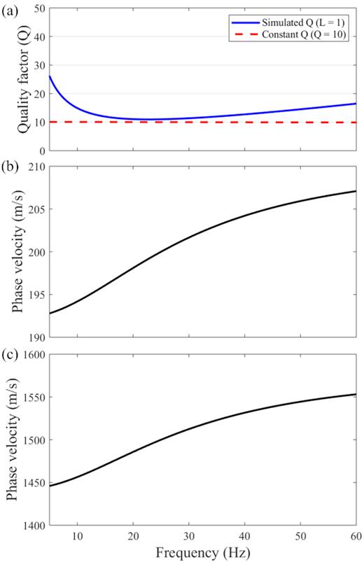
(a) Comparison of a constant Q value (red dashed line) and the Q values simulated by using one relaxation mechanism (blue solid line). (b) Phase velocity dispersion of VS = 200 m s−1 with ω0 = 2π · 25 Hz. (c) Phase velocity dispersion of VP = 1500 m s−1 with ω0 = 2π · 25 Hz.
2.2 Full-waveform inversion
Compared to the forward modelling equations (eqs 1–3), the adjoint state equations (eqs 8–10) only differ in the source terms and the sign before the spatial derivatives; therefore, they can be solved with the ‘same’ forward modelling code. Misfit gradients for parameters shear modulus, P-wave modulus, ρ, τS and τP are given in Fabien-Ouellet et al. (2017). Then the gradients in terms for VS, VP, ρ, τS and τP can be calculated by applying the chain rule on the Fréchet kernels.
3 SYNTHETIC EXAMPLES
In this section, we perform synthetic tests to explore the properties of 2-D multiparameter viscoelastic FWI. We first perform two multiparameter (five-parameters) examples by using a spatially uncorrelated and a spatially correlated model, respectively. Results of viscoelastic and elastic FWIs are also compared. Then we further investigate the crosstalk between coupled parameters VS and τS by comparing multiparameter (two-parameters) viscoelastic and mono-parameter elastic FWI results.
3.1 Multiparameter examples
We build a true model that consists of a depth-dependent 1-D background model. A triangular anomaly is superimposed on each parameter model at different positions (Fig. 2). Each triangular anomaly is 8 m wide and 4 m deep. The relative contrast between the anomaly and the background model in the Q models (e.g., QS = 10 compared with QS ≈ 80) is stronger than the contrasts in the velocity and the density models (e.g., VS = 120 m s−1 compared with VS ≈ 180 m s−1, ρ = 1850 kg m−3 compared with ρ ≈ 2100 kg m−3). We use a total of 10 shots with a source spacing of 10 m, starting from X = 20 m to X = 110 m. The vertical-force source is generated by a delayed Ricker wavelet with a central frequency of 30 Hz. We only use 10 shots to save computational cost. A total of 91 receivers (recording both vertical and horizontal components) are distributed along the free surface with an equidistant spacing of 1 m, starting from X = 20 m to X = 110 m. The 1-D background models are used as the initial models, and the true source wavelet is used during the inversion. We perform a multiparameter viscoelastic FWI on the synthetic data in which all five parameters are updated simultaneously during the inversion. A high-cut frequency filter of 25, 35, 45, and 60 Hz is used progressively in the multiscale strategy. A minimum of 15 iterations are performed at each stage, while the inversion moves to the next stage once the relative improvement in the misfit value becomes less than 1 per cent.
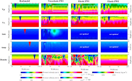
Multiparameter synthetic example on a spatially uncorrelated model. Four columns represent the true models, viscoelastic FWI results, elastic FWI results for both velocity and density models, and elastic FWI result for velocity models only, respectively. The 1-D background models are used as the initial models for the inversion. The red crosses represent the source locations. Blue and orange rectangles highlight the crosstalk between velocity models.
The reconstructed multiparameter models show a nice agreement with the true models (first and second columns in Fig. 2), especially for the velocity parameters VS and VP. On the contrary, the anomalies in the attenuation models are only roughly reconstructed. In the inverted τP model, the triangular anomaly cannot be identified. This reconstruction test shows that viscoelastic FWI is more sensitive to the velocities than the quality factors if we update all parameters simultaneously. Although the triangular anomaly can be easily identified in the reconstructed density model, the density model suffers strong crosstalk from the velocity models at the position where the VS and VP anomalies are located, respectively. Furthermore, the density model is also contaminated by strong fluctuations in the shallow part (depth < 4 m).
The reconstructed models show the interactions between the five parameters. VS has strong crosstalk to all the other parameters except for τP, and only weakly suffers crosstalk from VP and τS. VP has strong crosstalk to τP and density and suffers crosstalk mainly from VS. The attenuation and density models suffer strong crosstalk from both VS and VP but only weakly produces footprints to the other parameters. Overall, strong crosstalk mainly exists between VS and VP, from velocity to attenuation models of the same wave types (i.e. VS to τS, VP to τP), and from both velocities (VP, VS) to the density models.
In order to study the importance of considering attenuation, we perform an elastic FWI (Groos et al. 2014) with a fixed Q model on the same data set. Though named as elastic, the 1-D linear-gradient τ models are used in a viscoelastic forward solver but not updated during the inversion (it is sometimes also called ‘viscoelastic’, ‘pseudo-viscoelastic’, or ‘passive-viscoelastic’ FWI since a viscoelastic forward solver is used). Due to the high sensitivity of Rayleigh wave with respect to VS, the final VS model is recovered quite robustly. The VP model reconstructed by elastic FWI contains vertical-stripes artefacts (white square in Fig. 2, wavefront-like artefacts, since the Rayleigh waves mainly propagate horizontally with a vertical wavefront), which do not exist in the viscoelastic FWI result. Because the velocity parameter could not directly cause intrinsic damping in the data, we speculate that these vertical-stripped artefacts (scatterers) may arise to imitate the intrinsic anelastic damping by scattering attenuation (Wu 1985; Snieder 1988). The triangular shape of VP anomaly is less accurately delineated in the elastic FWI result compared to the viscoelastic result. The crosstalk (orange square, Fig. 2) between VP and VS becomes stronger in the elastic FWI results since it has fewer parameters to explain the data. Similar but weaker crosstalk can be observed in the reconstructed VS model (blue square, Fig. 2). This indicates that velocity models can be better recovered when considering the attenuation during the inversion. The density model contains strong artefacts in the shallow part (depth < 4 m) and is worse than the density model reconstructed by viscoelastic FWI. The final synthetic shot gathers in both the elastic and viscoelastic FWIs show a nice agreement with the observed data (Fig. 3a). The waveform residual in the viscoelastic FWI result is hardly visible and is smaller than the elastic FWI result (Figs 3b and c).
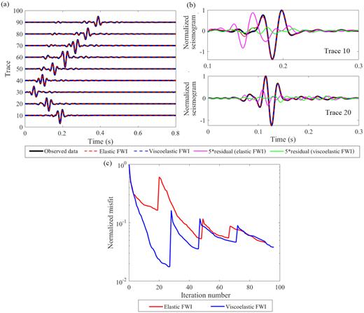
Data fitting in the synthetic example on the uncorrelated model (Fig. 2). (a) Comparison of the vertical velocity seismograms of the shot at X = 50 m. Thick black lines are the observed seismograms. Red and blue dashed lines are the synthetic seismograms corresponding to the inversion results of multiparameter elastic and viscoelastic FWIs, respectively. The waveform in each trace is scaled by its offset. (b) Upper and lower images show the zoomed comparison for trace 10 and trace 20, respectively. The waveform residual is magnified by five times. (c) Comparison of the data misfits in the elastic (red solid line) and viscoelastic (blue solid line) FWIs.
We conduct another elastic FWI by fixing both density and attenuation models, in which similar velocity models are estimated (fourth column, Fig. 2). It indicates that surface wave FWI is not very sensitive to the density model. Elastic and viscoelastic FWI produce similar VS models, indicating that VS can be recovered well if a smooth background Q model is used. However, the viscoelastic FWI results contain weaker artefacts in the secondary parameters such as VP and density, compared to the elastic FWI with passive attenuation model. Worse results in VS would be obtained if we would fully ignore attenuation effects and just perform purely elastic forward modelling in the FWI workflow (Groos et al. 2014).
In the second experiment, we assume that the parameter perturbations are located at the same position (first column, Fig. 4). This spatially correlated model is generally more realistic compared to the previous one since all the physical-parameter anomalies usually belong to the same geological target. The same acquisition geometry, initial models, and inversion parameters as in the first example are used. Similarly, we also perform both viscoelastic and elastic FWIs on the same data set for comparison.
Multiparameter synthetic example on a spatially correlated model. Three columns represent the true models, viscoelastic FWI results and elastic FWI results, respectively. The 1-D background models are used as the initial models for the inversion. All the colour scales are identical to Fig. 2. The red crosses represent the source locations.
All five parameter models are nicely reconstructed in the viscoelastic FWI results (second column in Fig. 4). The triangular shape of the anomaly is better delineated in the VS model compared to the VP model. We can see the location of the anomaly in both τS and τP with a more accurate estimation of the values compared with the spatially uncorrelated example. Although the anomaly is visible in the density model, it suffers from much stronger artefacts compared to the other parameter models.
The elastic FWI with fixed Q models also resolves the location and the velocity structure of the anomaly (third column in Fig. 4). The triangular shapes of both VP and VS anomalies (especially for VP), however, are worse delineated compared to the viscoelastic FWI results. The reconstructed density model shows a wrong result in which a high-density anomaly instead of the low-density anomaly is reconstructed. Similar to the previous example, both viscoelastic and elastic FWI nicely fit the observed data, while a smaller data misfit is obtained by viscoelastic FWI compared to elastic FWI (Fig. 5).
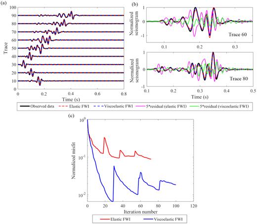
Data fitting in the synthetic example on the correlated model (Fig. 4). (a) Comparison of the vertical velocity seismograms of the shot at X = 50 m. Thick black lines are the observed seismograms. Red and blue dashed lines are the synthetic seismograms corresponding to the inversion results of multiparameter elastic and viscoelastic FWIs, respectively. The waveform in each trace is scaled by its offset. (b) Upper and lower images show the zoomed comparison for trace 60 and trace 80, respectively. The waveform residual is magnified by five times. (c) Comparison of the data misfits in the elastic (red solid line) and viscoelastic (blue solid line) FWIs.
Overall, both two synthetic experiments show that the reconstruction of VS is quite robust regardless of whether viscoelastic or elastic FWI is adopted. The viscoelastic FWI provides more accurate and comprehensive results compared to elastic FWI, especially for the reconstruction of VP. The reconstruction of attenuation is contaminated by the footprint from the velocity, while the velocity is relatively less affected by the attenuation.
3.2 Crosstalk between coupled velocity and quality factor
We perform another two synthetic tests to investigate the crosstalk between coupled parameters: VS and τS. We use the same 1-D background models for velocities and quality factors, but only superimpose a low-VS anomaly and a low-QS (high-τS) anomaly at different positions (first column, Fig. 6). We add a water table at 10 m depth, and the P-wave velocity below the water table is set to 1500 m s−1. A homogeneous density model with a value of 2050 kg m−3 is used. A total of seven vertical-force sources are placed with a spacing of 10 m from X = 20 m to X = 80 m. The sources are generated with a delayed Ricker wavelet of 30 Hz. A total of 61 two-component receivers are distributed along the free surface with an equidistant spacing of 1 m from the first to the last source positions. The 1-D background models are used as the initial models, and we only update VS and τS models during the inversion.
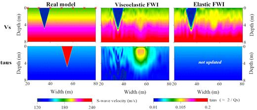
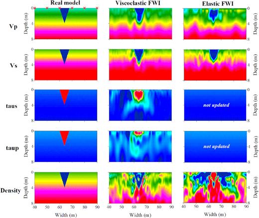
Two-parameter synthetic example on a spatially uncorrelated model. Three columns are the true models, two-parameter viscoelastic FWI results and monoparameter elastic FWI result, respectively. The red crosses represent the source locations.
In the spatially uncorrelated test, the reconstructed VS model by viscoelastic FWI (second column in Fig. 6) shows a nice agreement with the true model and is slightly affected by the τS anomaly. On the contrary, the τS model is only roughly reconstructed and the value of τS anomaly is underestimated. Besides, it is contaminated by a strong footprint from the VS anomaly. The poor reconstruction of the τS anomaly confirms the high sensitivity of VS.
For comparison, we perform an elastic FWI by adopting and keeping the background τS model during the inversion. The reconstructed VS model matches the true model satisfactorily (third column, Fig. 6). It clearly delineates the location, shape and the value of the VS anomaly. Nevertheless, the reconstructed VS model suffers stronger crosstalk from the τS anomaly compared to the result of viscoelastic FWI. Strong vertically orientated artefacts are also observed.
Similarly, we perform a synthetic test on a spatially correlated model in which VS and τS anomalies locate at the same location (first column in Fig. 7). Both VS and τS models are successfully recovered by viscoelastic FWI. In the result of elastic FWI, however, strong artefacts and distortion appear in the surrounding area of the anomaly (third column, Fig. 7). These artefacts behave as vertical-stripped anomalies, which are parallel to the wavefront of Rayleigh-wave. The shape of the τS anomaly is nicely delineated and more accurate compared to the spatially uncorrelated example. Overall, these two examples again show that the multiparameter viscoelastic FWI provides better result compared to the elastic FWI. If we do not invert for attenuation, the heterogeneity in QS may be projected into the reconstructed VS model.
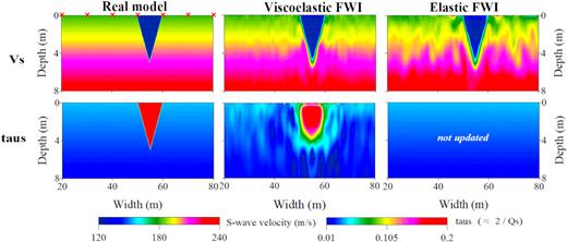
Two-parameter synthetic example on a spatially correlated model. Three columns are the true models, two-parameter viscoelastic FWI results and monoparameter elastic FWI result, respectively. The red crosses represent the locations of the sources.
4 APPLICATION TO FIELD DATA
We apply the multiparameter viscoelastic FWI strategy to a shallow seismic field data set. The test site is located on a glider airfield in Rheinstetten, Germany. The shallow subsurface is composed of fluviatile sediments from the late Pleistocene. A refilled trench, namely ‘Ettlinger Linie’ (EL), is approximately located in the middle of our survey line (Wittkamp et al. 2019). The seismic data set is excited by vertical hammer blows and recorded by 48 multicomponent geophones spaced every 1 m. Although multicomponent data outperforms single-component data in 2-D FWI (Nuber et al. 2017), we only use vertical-component data in our example because the horizontal-component data has a relatively low signal-to-noise ratio. A total of 12 shots with a 4-m spacing are used (asterisks in Fig. 8). The first source position is located between the first and second geophones. Furthermore, 3-D to 2-D transformation (Forbriger et al. 2014) is necessary before the FWI because we only use a 2-D forward solver. Schäfer et al. (2014) proved the applicability of this 3-D to 2-D transformation to heterogeneous models.
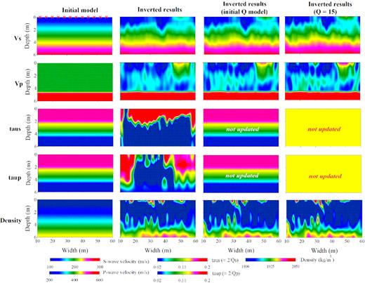
Comparison of reconstructed models in the field example. The first column represents the initial models. The second column shows the inversion results of multiparameter viscoelastic FWI. The third and fourth columns show the inversion results obtained by multiparameter elastic FWI without updating the Q models. The fixed Q models for the third and fourth columns are the depth-dependent and homogeneous Q models, respectively. The red crosses represent the locations of the sources.
We use surface wave methods to build the initial models for FWI to reduce the possibility of cycle skipping (first column in Fig. 8). 1-D VS and QS models are estimated by the inversions of Rayleigh-wave dispersion curve and attenuation coefficients (Gao et al. 2018), respectively. The initial 1-D VP model is estimated by first-arrival traveltime inversion. It consists of two layers with sharp velocity contrast at a depth around 6 m which corresponds to the groundwater table (Pasquet et al. 2015; Wittkamp et al. 2019). For the initial QP model QP = QS is assumed. A linear gradient model is used as the initial density model. The initial models are smoothed prior to FWI.
The multiscale strategy starts with low-pass filtered data up to 10 Hz. The frequency content is progressively increased by 5 Hz until 60 Hz is reached. A minimum of three iterations is guaranteed in each stage, and the inversion moves to the next stage when the relative decrease in the misfit value is less than 1 per cent. We estimate a wavelet correction filter by a stabilized deconvolution (Groos et al. 2014) and use it to update the source time function at the beginning of each stage.
The multiparameter inversion results are shown in the second column in Fig. 8. The inverted VS model shows a triangular low-velocity anomaly in the central part of the spread, indicating the existence and the location of the EL. A similar low-velocity anomaly can also be identified in the final VP model. The τS and τP models show relatively high τ values (low Q values with Q < 15) in the shallow subsurface (top 2 m), and relatively lower τ values (higher Q values) in the deeper part. It indicates that the attenuation in seismic waves is mainly caused by the shallow soil (weathering zone). The final density model doesn’t provide geological information about the trench, which may be caused by the relatively low sensitivity of Rayleigh waves with respect to density. Overall, the inversion of the field data provides a relatively high resolution in the velocity models and a relatively low resolution in the Q and density models. Twelve inverted source time functions (Fig. 9) show a similar shape among each other, indicating that estimated source time functions are fairly reliable. It is worth mentioning that the final wavelet does not necessarily represent the actual source wavelet excited in the field measurement, instead, it also accounts for the residual caused by the inaccurate inversion result. The synthetic waveforms fit the observed data fairly well (Fig. 10), which indicates a successful explanation of the observed wavefield by the final multiparameter models.
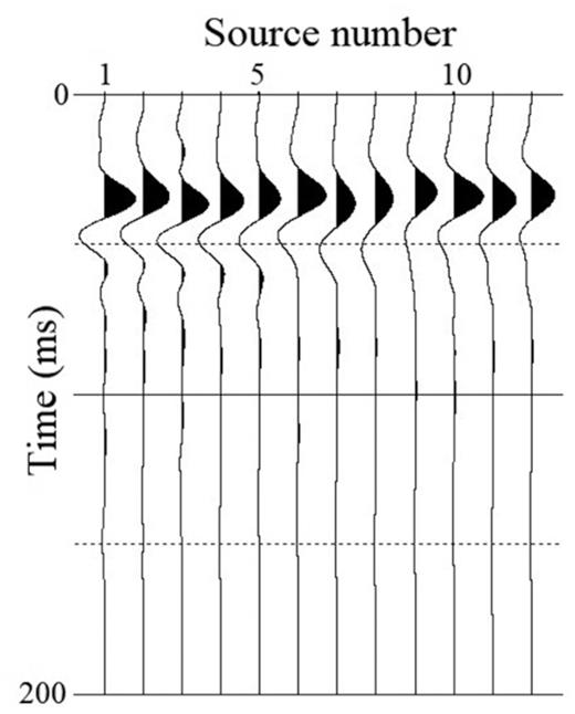
The estimated source time functions of the 12 shot gathers.
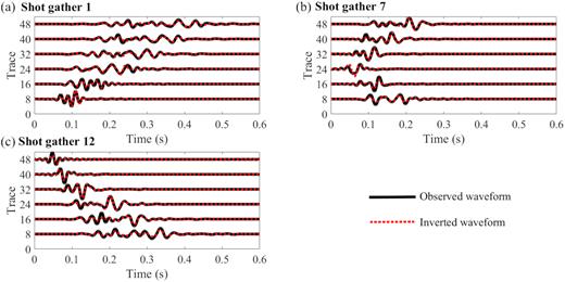
Comparison of vertical velocity seismograms in the first, seventh and last shots. Thick black lines are the observed seismograms. Red dashed lines are the synthetic seismograms corresponding to the inversion results of multiparameter viscoelastic FWI. The waveform in each trace is scaled by its offset.
In order to study the role of attenuation for the Rheinstetten study area, we also perform elastic FWI tests on the same data by using a fixed initial depth-dependent Q model and a homogeneous Q model during the inversion (third and fourth columns in Fig. 8), respectively. The inverted VS and VP models show a similar low-velocity anomaly. However, they are contaminated with vertical-striped artefacts, which is mainly caused by ignoring the heterogeneity in the Q models. Similar artefacts have also been observed in our synthetic reconstruction tests. The existence of the artefacts makes it difficult to identify the shape of the EL in the reconstructed P-wave velocity model.
To validate our final FWI results, we compare our velocity models obtained by viscoelastic FWI (second column in Fig. 8) to a migrated GPR profile (Wittkamp et al. 2019) acquired along the same survey line (Fig. 11). The comparison with the GPR section shows a fairly good agreement concerning the location and the shape of the EL. It verifies fairly high reliability of the final S- and P-wave velocity models estimated by the multiparameter viscoelastic FWI.

Comparison between the field-data inversion results and a GPR profile. The S- and P-wave velocity models are overlying on the migrated image of the GPR measurement.
5 DISCUSSION
In the field-data application, the elastic FWIs also nicely reconstruct the S-wave velocity models because we adopt good passive Q models in the elastic FWI. It indicates that the availability of a sufficiently good passive Q model allows the reconstruction of a reliable S-wave velocity model. Poorer results will be obtained if we use the purely elastic FWI without any prior information of attenuation (Groos et al. 2014). Nevertheless, the numerical tests show that, when encountering heterogeneous Q model, multiparameter viscoelastic FWI can further improve the accuracy of estimated velocity model and is superior to elastic FWI in which attenuation is considered as a passive modelling parameter only. In our field example, a similar improvement in the accuracy of the inversion result is also observed, especially for the reconstruction of the P-wave velocity model. Besides, the reconstructed Q models might also be helpful for geological interpretation. Therefore, it is meaningful to incorporate attenuation into the inversion for reconstructing accurate multiparameter results to better delineate the subsurface structures and properties, especially when the Q model is highly heterogeneous.
In general, the resolution of the estimated Q models in viscoelastic FWI is much poorer compared to the resolution of the velocity models. Only one relaxation mechanism has been used in this study to describe the frequency dependency of Q for the sake of computational cost. Since we only use single relaxation mechanism, the estimated Q values might be lower than their true values (Fig. 1). The importance of considering multiple relaxation mechanisms needs to be further investigated in the future.
Multiparameter inversion including seismic velocities and quality factors of both P and S waves can provide more comprehensive information to improve the characterization of the shallow subsurface. However, the inversion results might be contaminated by crosstalk between the perturbations of different parameters, which decreases the reliability of the reconstructed models. In this paper, we use a preconditioned conjugate gradient algorithm to invert the data, which cannot reduce the parameter trade-off between coupled parameters appropriately. The utilizing of second-order optimization algorithm (Operto et al. 2013; Métivier et al. 2013) for reducing parameter trade-offs in the viscoelastic FWI of shallow-seismic data needs to be further investigated.
6 CONCLUSIONS
We applied 2-D multiparameter viscoelastic FWI to shallow-seismic surface waves. We tested the capability of this method to reconstruct reliable parameters on synthetic data sets with spatially correlated and uncorrelated models. The synthetic results of spatially uncorrelated models showed that shallow-seismic data has the highest sensitivity with respect to VS, then VP, and relatively low sensitivity to density, QS and QP. They also showed that crosstalk mainly exists between velocity models (i.e. VS and VP) and coupled velocity–quality factor pairs (i.e. VS and QS, VP and QP). Crosstalk between coupled parameters VS and τS was further investigated by another two synthetic examples in which strong crosstalk from VS to τS is observed. If attenuation is not updated, artefacts in the estimated velocity models may be developed. Overall, all these synthetic examples showed that multiparameter viscoelastic FWI provides more accurate and comprehensive multiparameter results compared to the elastic FWI, especially for the reconstruction of the P-wave velocity model.
We also applied the multiparameter viscoelastic FWI approach to a field shallow-seismic data set acquired in Rheinstetten, Germany. The final VS and VP models revealed a sharp triangular low-velocity anomaly, which accurately delineates the location and the shape of a known refilled trench. We compared our viscoelastic FWI result to the results estimated by elastic FWI in which Q models were included but not updated during the inversion. Although the elastic results could also reveal the triangular low-velocity anomaly in the VS models, they were contaminated by vertical-striped artefacts, which was mainly caused by the neglecting of heterogeneity in the Q models. A good agreement between our viscoelastic FWI result and a migrated GPR profile verified the accuracy of our estimated models and the validity of the method. Mitigation of crosstalk between coupled parameters needs to be studied in the future.
ACKNOWLEDGEMENTS
The authors thank the editor Hervé Chauris and two anonymous reviewers for their constructive comments. This work was funded by the Deutsche Forschungsgemeinschaft (DFG, German Research Foundation)—Project ID 258734477–SFB 1173.
REFERENCES
Author notes
The first two authors contributed equally to this work.
