


SUMMARY
We report finite-frequency imaging of the global 410- and 660-km discontinuities using boundary sensitivity kernels for traveltime measurements made on SS precursors. The application of finite-frequency sensitivity kernels overcomes resolution limits in previous studies associated with large Fresnel zones of SS precursors and their interferences with other seismic phases. In this study, we calculate the finite-frequency sensitivities of SS waves and their precursors based on a single-scattering (Born) approximation in the framework of travelling-wave mode summation. The global discontinuity surface is parametrized using a set of triangular gridpoints with a lateral spacing of about 4°, and we solve the linear finite-frequency inverse problem (2-D tomography) based on singular value decomposition (SVD). The new global models start to show a number of features that were absent (or weak) in ray-theoretical back-projection models at spherical harmonic degree l > 6. The thickness of the mantle transition zone correlates well with wave speed perturbations at a global scale, suggesting dominantly thermal origins for the lateral variations in the mantle transition zone. However, an anticorrelation between the topography of the 410-km discontinuity and wave speed variations is not observed at a global scale. Overall, the mantle transition zone is about 2–3 km thicker beneath the continents than in oceanic regions. The new models of the 410- and 660-km discontinuities show better agreement with the finite-frequency study by Lawrence & Shearer than other global models obtained using SS precursors. However, significant discrepancies between the two models exist in the Pacific Ocean and major subduction zones at spherical harmonic degree >6. This indicates the importance of accounting for wave interactions in the calculations of sensitivity kernels as well as the use of finite-frequency sensitivities in data quality control.
1 INTRODUCTION
The 410- and 660-km discontinuities have been progressively mapped out in global seismic imaging since the 1990s (Revenaugh & Jordan 1991; Shearer 1991; Flanagan & Shearer 1998; Gu et al. 1998, 2003; Lawrence & Shearer 2006; Deuss 2009). High temperature and pressure mineral physics experiments suggest that the two discontinuities are associated with pressure-induced phase transitions of olivine to wadsleyite at about 410 km and ringwoodite to perovskite + magnesiowustite at about 660 km, respectively (Anderson 1967; Ita & Stixrude 1992). In regional and local seismic imaging, P-to-S converted waves have been widely used to map the two discontinuities at relatively high resolutions, especially in regions where seismic data have been recorded by small aperture arrays (Shen et al. 1998; Li & Yuan 2003; Lee et al. 2014; Gao & Liu 2014; Kosarev et al. 2017; Kaviani et al. 2018; Zhou 2018). In general, global models obtained using P-to-S converted waves have lower resolution in oceanic areas because of limited data coverage (Chevrot et al. 1999; Lawrence & Shearer 2006). In global studies, the underside reflections of SS waves (SS precursors) have been used to map the global depth perturbations of the 410 and the 660. SS precursors are most sensitive to discontinuity structures near the SS wave bounce points and therefore they provide better global coverage than P-to-S converted waves, especially in oceanic regions where very few seismic stations are deployed.
SS precursors are secondary waves reflected at the underside of the 410-km and the 660-km discontinuities, their amplitudes are relatively small due the low impedance ratio across the two seismic discontinuities (Fig. 1). Previous SS precursor studies in imaging the global mantle transition zone structures commonly chose to stack the SS precursors in large circular bins to improve the signal-to-noise ratios and obtain depth perturbations on the discontinuities based on the conventional JWKB ray theory (Shearer 1991; Gu et al. 1998, 2003; Schmerr & Garnero 2006; Houser et al. 2008; Deuss 2009). Ray theory is a high-frequency approximation which assumes that seismic waves travel through the earth along infinitesimally narrow paths. In reality, however, seismic waves have finite frequency and SS waves are sensitive to a large area on the boundary centered at the bounce point. It has been suggested by several studies that topographic structures with sizes smaller than the first Fresnel zone may not be resolved properly using the traditional ray theory (Neele et al. 1997). The resolution of the ray-theoretical models is limited by the large Fresnel zone of SS waves and their precursors (∼1000 km at 20-s period) and only large-scale features are reliable. A better theory, which can account for scattering, wave front healing and other finite frequency effects of seismic waves is needed to improve the resolution of smaller scale topographic anomalies. Neele & de Regt (1999) proposed a method to approximate the finite-frequency sensitivities of SS and PP precursors over the first Fresnel zone. They applied the method to a large synthetic data set and showed that depth variations with a lateral scale smaller than the first Fresnel zone but larger than the dominant wavelength can be well resolved. The first global topographic maps of the 410 and the 660 based on finite-frequency theory were published by Lawrence & Shearer (2008) using traveltime sensitivity kernels of SS precursors calculated based on ray tracing (Dahlen 2005). The power spectra of the seismic phases in the reference model were approximated by the observed power spectra, and, the sensitivity kernels were stacked in circular bins of different sizes in the inversions.
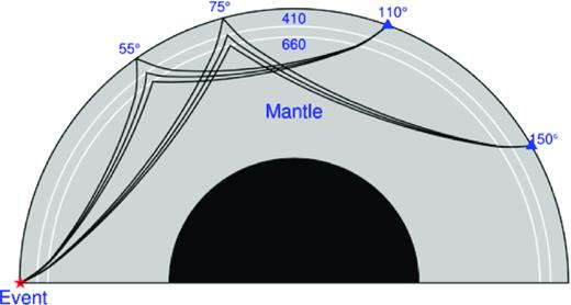
Ray paths of SS, S410S and S660S waves at epicentral distances of of 110° and 150°. The star and triangles indicate locations of the earthquake event and the recording stations, respectively.
In this study, we construct a global data set of finite-frequency traveltime measurements of SS waves and SS precursors by measuring traveltime differences between the observed and synthetic seismograms in the frequency domain. One major concern in imaging the 410 and the 660 using SS precursors is phase interactions (e.g. precursors of ScSScS wave and the postcursors of Sdiff interfere with SS precursors). To reduce possible uncertainties in SS precursor data, earlier studies often chose to to limit the range of epicentral distance to avoid possible phase interference, which limits the spatial resolution of available data (Schmerr & Garnero 2006; Deuss 2009; Lessing et al. 2014). To overcome the above limitations, we calculate sensitivity kernels in the framework of travelling-wave mode coupling, which fully accounts for interference of seismic waves arriving in the measurement windows, the effects of source radiation and seismogram windowing/tapering. This study is the first study to image the 410- and 660-km discontinuities using single-trace SS (and precursor) traveltime measurements and individual finite-frequency sensitivity kernels.
The sensitivity kernels can be used to identify measurements that are heavily influenced by shallower multiples, and, those measurements can be excluded when they are not most sensitive to the depth perturbations of the 410 and the 660. We will focus on finite-frequency effects in the imaging of the 410 and the 660 using single trace traveltime measurements of SS precursors by investigating models obtained using 2-D diffractional tomography and those obtained from ray-theoretical back-projections using the the same data set. We compare our finite-frequency discontinuity model with previous studies and show that the new model agrees better with the finite-frequency model by Lawrence & Shearer (2008) than other global models imaged using SS precursors based on ray theory. We will discuss major discrepancies between the two finite-frequency models and the significance of data processing in finite-frequency imaging.
2 FINITE-FREQUENCY TRAVELTIME MEASUREMENTS
We built a global data set of the finite-frequency traveltime measurements using seismograms recorded at 150 stations in the Global Seismological Network (GSN) for earthquakes that occurred between January 2003 and September 2014 (Fig. 2). The earthquakes have moment magnitudes ranging from 6.0 to 8.5 and focus depths less than 100 km. All available seismograms with epicentral distances between 90° and 160° are downloaded from the Data Management Center at the Incorporated Research Institutions for Seismology (IRIS). Initial data processing includes removing instrument responses, rotating the horizontal components to obtain the transverse component seismograms and applying bandpass filter with corner frequencies at 0.01 and 0.1 Hz. We visually inspected seismograms and carefully selected the ones with high signal-to-noise ratios and clear SS waves and precursors. We corrected abnormal polarities of the transverse component seismograms at several stations and we discarded seismograms with highly deformed SS waveforms. The final data set contains a total number of about 6400 seismograms from 1117 earthquakes.
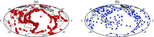
(a) Distribution of 1117 teleseismic earthquakes (6.0 < Mw < 8.5) used in this study. The epicentral distance of the data set ranges from 90° to 160°. (b) Locations of 150 GSN stations used in this study.
Synthetic seismograms are calculated in a 1-D reference earth model IASP91 (Kennett & Engdahl 1991) based on travelling-wave mode summation up to 0.2 Hz (Liu & Zhou 2016). The global centroid-moment-tensor (CMT) solution and the USGS Preliminary Determination of Epicenters (PDE) source locations and origin times are used in the calculations of the 1-D synthetic seismograms. The same bandpass filter is applied to the synthetic seismograms. We manually pick measurement windows centered near the maximum amplitudes of the phases (SS or SS precursors) and the length of the measurement time windows ranges from 70 to 120 s. Finite-frequency traveltime measurements are made with a cosine taper of the same length to limit spectra leakage (Fig. 3). The spectrum of the cosine taper shows a relatively broad central peak and very weak side lobes (Deng & Zhou 2015). The differences in traveltimes between the synthetic and observed signals are calculated in the frequency domain (Xue et al. 2015).
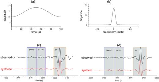
Panels (a) and (b) are a 100-s cosine taper in the time domain and its spectrum in the frequency domain, respectively. Panels (c) and (d) are example observed and synthetic seismograms with clear SS, S410S and S660S waves, recorded at station EFI for an Indonesia earthquake occurred on 26 May 2003 (Mw = 6.9) and at station LBTB for a Mexico earthquake occurred on 22 January 2003 (Mw = 7.5), respectively. The shaded areas indicate time windows used for traveltime measurements.
Fig. 3 shows examples of observed and synthetic seismograms from the data set. The observed seismogram in (c) is recorded at station EFI on East Falkland Island from a moment magnitude 6.9 earthquake in Indonesia, and the observed seismogram in (d) is recorded at station LBTB from a moment magnitude 7.5 earthquake in Mexico. The epicentral distances are 130° and 133°, respectively. Time windows used for measuring the traveltime residuals of SS waves and SS precursors are shaded on the seismograms. It is important to point out that finite-frequency traveltime measurements depend on the length and position of the measurement windows as well as the time-domain taper applied in making the measurements. The effects of windowing and tapering are accounted for in the calculation of the finite-frequency sensitivity of each measurement. In this paper, we will focus on inversions using data obtained at a measurement period of 20 s.
3 FINITE-FREQUENCY SENSITIVITIES TO BOUNDARY PERTURBATIONS
Fig. 4 shows examples of 2-D traveltime sensitivity of S410S and S660S waves to depth perturbations of the 410- and 660-km discontinuities. The epicentral distance is 133° and the kernels are calculated for traveltime measurements at a period of 20 s. The sensitivity kernels show the typical X shape with maximum positive values in the center of the X and alternating side bands in the second and third Fresnel zones. The size of the first Fresnel zone (with positive sensitivity) is about 15° × 15°, indicating that ray theory, which assumes traveltime sensitive only to structure at the bounce point, is a rather crude approximation in this case.
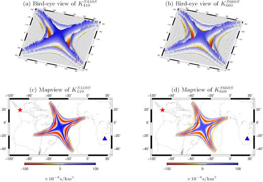
(a) Bird-eye view of example finite-frequency sensitivity of an S410S wave at a period of 20 s to depth perturbations of the 410-km discontinuity. The epicentral distance is 133° and the mapview of the sensitivity kernel is plotted in (c) where the earthquake (star) is located off the west coast of Mexico and the station LBTB (triangle) is in Africa. The sensitivity of the corresponding S660S to depth perturbations on the 660-km discontinuity is plotted in (b) and (d).
In general, the boundary sensitivity of SS waves is about an order of magnitude smaller than the sensitivity of SdS waves (Fig. 5). Therefore, the sensitivity kernels of the SdS−SS differential measurements show only minor differences from the SdS sensitivity kernels. We point out that the boundary sensitivity kernels are associated with measurement time windows, which may include multiple phases arriving closely in time. Therefore, they often have structures more complex than those plotted in Figs 4 and 5 due to interfering seismic phases. For those measurements, the typical X-shape structure due to the minimum-maximum nature of the precursors will be deformed and the amplitudes of the sensitivity may become extreme. The complexity of the finite-frequency sensitivity kernels can be used to identify measurements associated with wave interference due to multiples of a shallower interface or other seismic phases. We exclude those measurements as linear perturbation theory may not apply when the reference phase is much weaker than scattered waves.
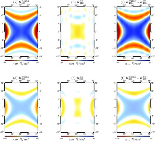
Zoom-in view of sensitivity kernels of S410S, S660S and SS waves recorded at station BJT (longitude = 116.17°, latitude = 40.02°) with an epicentral distance of 120° from a Mw 6.3 earthquake in Puerto Rico area. The SS sensitivities are much smaller in magnitude and plotted on difference color scales. SdS and SS waves have different sensitivity polarity as a depression of the 410-km (or 660-km) discontinuity will speed up SdS waves but slow down SS waves, and vice versa for an uplift.
4 THE INVERSE PROBLEM
5 FINITE-FREQUENCY EFFECTS IN DISCONTINUITY IMAGING
The 410- and 660-km discontinuity models obtained from finite-frequency inversions are plotted in Fig. 6. We have removed the mean perturbations of the two discontinuities and the reference depths of the 410-km and the 660-km discontinuities in Fig. 6 are 411.6 and 660.4 km, respectively. Positive perturbations (in blue) indicate discontinuity depths greater than the reference depths, and negative perturbations (in red) indicate shallower discontinuity. Overall, the 660-km discontinuity shows larger depth variations than the 410-km discontinuity, which is consistent with traveltime observations. The S660S and S410S measurements have similar standard deviations (6.14 and 6.10 s, respectively) while the same amount of depth perturbations on the two discontinuities would predict larger traveltime anomalies in the S410S waves than the S660S waves. Stronger topographic variations of the 660-km discontinuity have also been observed in several previous studies (Flanagan & Shearer 1998; Gu et al. 2003; Lawrence & Shearer 2008).
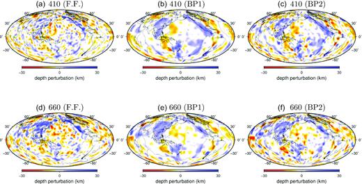
Finite-frequency effects in imaging depth perturbations of the 410-km and the 660-km discontinuities. Panel (a) depth perturbations of the 410-km discontinuity inverted from SdS–SS traveltime measurements using finite-frequency sensitivity kernels. Panels (b) and (c) are ray-theoretical back-projection models where perturbations are averaged in a moving circular cap with a radius of 6° (BP1) and 4° (BP2). Panels (d)–(f) are the finite-frequency and ray-theoretical back-project models for depth perturbations on the 660-km discontinuity. The finite-frequency model and ray-theoretical back-project models are obtained using the same traveltime data without crustal and mantle wave speed corrections.
The 660-km discontinuity is overall shallower in oceanic regions and deeper in a broad region across the Eurasia and along the west coast of the North America. Regional studies using receiver functions and PP/SS precursors have reported similar depressed 660 topography in the Sea of Okhotsk, Eastern Russia, Northeastern China as well as the North American Farallon subduction zone (Heit et al. 2010; Schmerr & Thomas 2011; Gao & Liu 2014; Zheng et al. 2015; Wang & Pavlis 2016; Zhou 2018). The 660-km discontinuity beneath the Mediterranean Sea and the Middle East shows several small-scale depressions which were also imaged by Kaviani et al. (2018).
The ocean–continent contrast is much weaker on the 410-km discontinuity. There is an apparent age-dependent signature in the Pacific Ocean, where the 410 becomes deeper towards the middle ocean spreading centers. The 410-km discontinuity is depressed in the western North America and eastern Asia extending from Tibet through central and northern China to the western Sea of Okhotsk, in general agreement with regional studies (Heit et al. 2010; Gao & Liu 2014; Wang & Pavlis 2016).
In Fig. 6, we compare the finite-frequency models of the 410- and 660-km discontinuities with depth perturbations obtained from back-projection using the same SdS–SS traveltime measurements. In ray-theoretical data back projection, we do not invert the traveltime measurements but estimate discontinuity depth perturbations from traveltime residuals using 1-D time-depth derivatives. The depth perturbations are averaged in a moving circular cap with a constant radius and plotted in Fig. 7. When the cap size is small (4°), the resulting back-projection maps become more noisy due to rather small number of data points available in the averaging cap, especially in South America and Western Australia where data sampling is sparse. For example, extreme values in isolated regions in South America and Eastern North America in Fig. 6(c) are a result of unsuppressed noise in data due to insufficient averaging. When the radius of the cap is 6°, the structure becomes more smooth. Overall, the long-wavelength structures of the 410- and 660-km discontinuity maps obtained using ray-theoretical data back projection agree well with finite-frequency models.
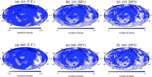
Panel (a) is the sensitivity density (diagonal elements of the matrix ATA) in finite-frequency tomography of the 410-km discontinuity. Panels (b) and (c) are the number of traces per circular cap in the back-projection models BP1 and BP2, respectively. Panels (d)–(f) are the same as (a)–(c) but for the 660-km discontinuity models in Fig. 6.
In Fig. 7, the finite-frequency sensitivity density and the back-projection ray density show similar coverage and smoothness when the size of the circular cap used in ray-theoretical back projection is 6°. The resulting models show large discrepancies in their dominant structure length scales (Fig. 6). The finite-frequency models show much stronger small-scale structures that are absent in the ray-theoretical back-projection models. In regions where data coverage is sparse, depth perturbations are very small, indicating that the finite-frequency models have been adequately damped (Figs 7 and A1). The stronger small-scale structures are expected as finite-frequency sensitivity kernels account for wave diffractional effects. For example, the anomalies along the western North America are much narrower and mostly confined in the continent regions while anomalies are much broader and diffused in the ray-theoretical back-projection models, regardless of the cap size.
We calculate the correlation coefficients between the finite-frequency models and the back-projection models as a function of spherical harmonic degree up to l = 20 in Fig. 8. Models obtained using finite-frequency tomography and ray-theoretical back projection are positively correlated at all spherical harmonic degrees, regardless of the averaging cap size. The two 410-km discontinuity models are well correlated with a correlation coefficient of 0.96 in their large-scale structures (l < 5), and the correlation coefficient decreases to ∼0.8 at intermediate length scales (6 ≤ l ≤ 14). For smaller scale structure with harmonic degree l ≥ 15 (wavelength <∼2500 km), the correlation coefficient decreases to ∼0.5. The correlation between the two 660-km discontinuity models show very similar variations as a function of spherical harmonic degree, except that small-scale structures show better correlations with the finite-frequency model when a 4° cap is used in the back-projection model.
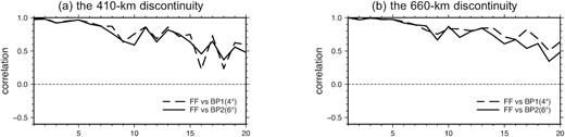
(a) Correlation coefficient as a function of spherical harmonic degree between the finite-frequency 410-km discontinuity model and the two back-projection models in Fig. 6. (b) Same as (a) but for the 660-km discontinuity models.
6 CRUST AND MANTLE CORRECTIONS
Lateral variations in crustal structure and seismic wave speed in the upper mantle will introduce traveltime differences between observed and synthetic seismograms calculated in the 1-D reference earth model, IASP91 (Kennett & Engdahl 1991). These traveltime anomalies can be subtracted from SS and SdS measurements by applying corrections using published 3-D crust and mantle velocity models. In this section, we investigate the impact of crustal and mantle corrections on the imaging of the 410- and 660-km discontinuities in finite-frequency tomography. We calculate expected traveltime anomalies caused by the 3-D structure of the crust using a global crustal model CRUST1.0 (Laske et al. 2013). This is a 1° × 1° model which parametrized wave speeds and density in the crust and uppermost mantle as 8 layers in every 1° × 1° cell. Crustal corrections are positive beneath continents and negative in oceanic areas. The maximum correction is about 4.6 s for SS waves with bounce points in the Tibetan Plateau where the crust is about 60 km thicker than in the reference model.
Mantle wave speed corrections are often applied to account for traveltime anomalies caused by 3-D wave speed structure in the mantle using global models from independent studies. This method has been suggested to be more straightforward and accurate in SS precursor imaging than joint inversions to resolve discontinuity depth variations and wave speed perturbations simultaneously (Houser et al. 2008). This is because data sets required to image discontinuity depths are different from those that constrain seismic wave speed in the bulk mantle, including surface waves, body waves and free oscillations (Panning & Romanowicz 2006; Zhou et al. 2006; Ritsema et al. 2011; Schaeffer & Levedev 2013; Moulik & Ekstrom 2014). We calculate traveltime corrections using two different global 3-D mantle models, S40RTS (Ritsema et al. 2011) and S362ANI+M (Moulik & Ekstrom 2014). In model S40RTS, wave speed perturbations are with respect to a 1-D reference earth model PREM (Dziewonski & Anderson 1981) while the 3-D model S362ANI+M is anisotropic and wave speed perturbations are deviations from a 1-D reference model STW105 (Kustowski et al. 2008). Wave propagation simulations in 3-D earth models using the spectral element method have shown that traveltime corrections based on ray theory are adequate for wave speed models obtained using ray theory (Deng & Zhou 2015), we calculate wave speed perturbations in S40RTS and S362ANI+M with respect to the same 1-D reference model IASP91 and then integrate traveltime anomalies along the ray paths of SS waves and SS precursors. In general, wave speed corrections for SdS–SS measurements are smaller than that for individual SS and SdS waves, which is not unexpected as wave speed structure in the lower mantle introduces similar shifts in both the SS and SdS traveltimes.
The absolute traveltime corrections are significant with maximum values up to 15–20 seconds for some paths, but the corrections do not change the general geographic pattern of the SdS–SS traveltime residuals when plotted at the SS-wave bounce points (Fig. 9). However, the corrections do affect the amplitudes and the exact locations of the discontinuity anomalies in the final models (Fig. 10). For example, the age-dependent depth perturbation of the 410-km discontinuity in the Pacific Ocean in Fig. 6 becomes much weaker after wave speed corrections are applied. In addition to oceanic regions, crustal and mantle corrections also have an impact on discontinuity structures beneath stable cratons (e.g. the Canadian shield and the Baltic Shield) where the magnitude of SdS–SS traveltime measurements is either reduced or changes polarity after crustal and mantle wave speed corrections (Fig. 10). This can be explained by early arrivals of SS waves associated with increased wave speed in the upper mantle in those regions. The strong discontinuity anomalies beneath California also become much weaker after the corrections are applied. It is noteworthy that traveltime corrections made using different global mantle waves peed models (S40RTS versus S362ANI) are highly correlated and the final models after wave speed corrections do not show major differences (Figs 10 and 11).
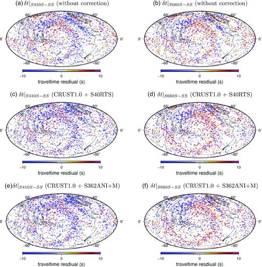
Panels (a) and (b) are S410S-SS and S660S-SS differential traveltime measurements at a period of 20 s without crustal and mantle corrections. The measurements are plotted at the bounce points of SS waves. Panels (c) and (d) are the same as (a) and (b) but with data corrected for crustal and mantle wave speed variations using models CRUST1.0 and S40RTS. (e) and (f) are the same as (c) and (d) but with mantle corrections using model S362ANI+M.
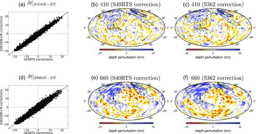
(a) Scatterplot of S410S−SS differential traveltime measurements with mantle corrections made using model S40RTS (Ritsema et al. 2011) and model S362ANI+M (Moulik & Ekstrom 2014). Panels (b) and (c) are depth perturbations of the 410-km discontinuity from finite-frequency tomography with traveltime corrections made using model S40RTS and S362ANI+M, respectively. Panels (d)–(f) are the same as (a)–(c) but for the 660-km discontinuity.
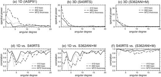
(a) Spectra power per spherical harmonic degree of the finite-frequency 410- and 660-km discontinuity models in Fig. 6 and the corresponding mantle transition zone thickness. (b) and (c) are the same as (a) but for discontinuity models in Fig. 10 where traveltime corrections have been made using model S40RTS and S362ANI+M, respectively. (d) Correlation coefficients as a function of spherical harmonic degree between the discontinuity models obtained with and without corrections based on model S40RTS (Figs 6 and 10). (e) is the same as (d) for models with and without traveltime corrections made using model S362ANI+M. Panel (f) correlation coefficients between models obtained with corrections made using models S40RTS and S362ANI+M.
The impact of crustal and mantle wave speed corrections on discontinuity structures at different length scales are plotted in Fig. 11. In spherical harmonic analysis, the power spectra is expected to decrease rapidly with angular degree when the peak amplitude of lateral variations remains the same. For example, the spectra power at degree l = 2 is about one order of magnitude larger than the spectra power at degree l = 12 when depth perturbations at the two harmonics degrees have the same peak amplitude. In general, crustal and mantle corrections emphasize low spherical harmonic degree structures in the discontinuity maps (Figs 10 and 11). For example, the maximum spectra power of the 660-km discontinuity map is at degree l = 2 without data corrections, while the degree-one (l = 1) structure becomes the strongest after crustal and mantle wave speed corrections are applied. This leads to low correlation coefficients between models obtained with and without corrections at degrees 1–2. The correlation is positive but weak at degrees l = 4−5 and increases with spherical harmonic degree with strongest correlations at degrees l ≥ 8 (length scale ≤2500 km). The thickness of the mantle transition zone is least sensitive to crust and mantle wave speed corrections and is strongly correlated between models with and without the corrections. Overall, the discontinuity models with and without crust and mantle wave speed corrections are well correlated regardless of the 3-D wave speed model used in making the corrections.
7 DISCONTINUITY TOPOGRAPHY AND WAVE SPEED STRUCTURE
The Clapeyron slope, which is the change in pressure over the change in temperature dP/dT, is positive for the olivine to wadsleyite phase transformation (the 410-km discontinuity) and negative for the ringwoodite to perovskite and magnesiowustite phase transformation (the 660-km discontinuity). If undulations of the two discontinuities are dominantly caused by lateral thermal variations in the mantle transition zone, we would expect a negative correlation between the 410 topography and variations in seismic wave speed. For example, in regions where cold slab materials reside in the mantle transition zone, seismic wave speed increases while the depth of the 410-km discontinuity decreases, resulting in a negative correlation. In contrast, the correlation between wave speed and discontinuity depth would be positive for the 660-km discontinuity due to its opposite Clapeyron. Examining the correlations between perturbations in wave speed and discontinuity depth will in turn allow us to investigate dominant mechanisms responsible for depth perturbations of the 410- and 660-km discontinuities.
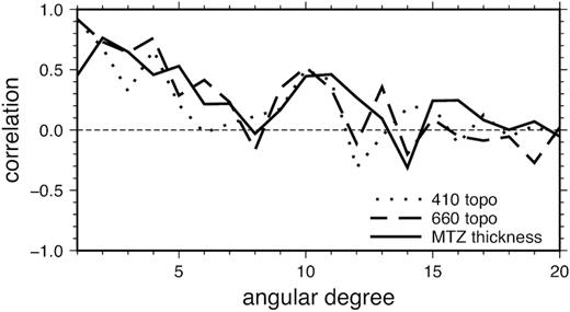
In Fig. 12, we investigate the correlation between discontinuity depth perturbations and seismic wave speed variations in the mantle transition zone using a global model S40RTS (Ritsema et al. 2011). The discontinuity models are obtained from traveltime data with corrections made using the same wave speed model. There is no clear correlation between the topography of the 410-km discontinuity and wave speed variations at a global scale, except for at spherical harmonics degree l = 4 (length scale of ∼5000 km) where the correlation is positive. The absence of an overall negative correlation between seismic wave speed and the 410-km discontinuity suggests possible non-thermal origin of heterogeneities. For example, heterogeneities in chemical composition or changes in water content (Schmerr & Garnero 2007; Gu et al. 2014; Wang et al. 2017).
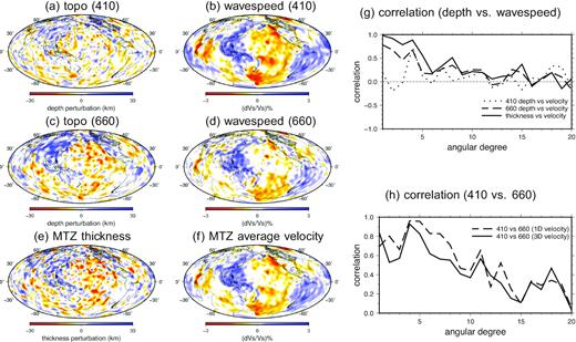
Panels (a) and (c) are the finite-frequency 410- and 660-km discontinuity models with data corrections made using model S40RTS (Fig. 10). Panels (b) and (d) are wave speed perturbations in model S40RTS at depths of 410 and 660 km, respectively. Panels (e) and (f) are maps of the mantle transition zone thickness and average wave speed in the mantle transition zone, respectively. Panel (g) correlation between discontinuity depth perturbations and wave speed perturbations as a function of spherical harmonic degree; (h) correlation between the 410- and 660-km discontinuity models in 1-D (no correction) and 3-D (with correction) wave speed models.
The topography of the 660-km discontinuity, on the other hand, shows clear positive correlations with seismic wave speed in the mantle transition zone up to spherical harmonic degree l = 11 (length scale of ∼3600 km). This positive correlation supports a thermal origin at a global scale. The correlation becomes weaker at higher spherical harmonic degrees and no apparent correlation is observed at l > 15 (lengthscale∼1300 km), which is likely due to different lateral resolutions in the wave speed and topography models. This change from no (weak) correlation at 410 km depth to significant positive correlation at 660 km depth may also be a result of limitations in depth resolution of the global seismic wave speed model over a scale of 250 km in the mantle transition zone.
The thickness of the mantle transition zone shows strongest correlation with seismic wave speed. This positive correlation is not surprising as variations in thickness are dominated by the depth perturbations on the 660-km discontinuity, and, there is a positive correlation between the 660-km discontinuity topography and seismic wave speed. The correlation is stronger in long wavelength variations at spherical harmonic degree l < 8. Geographically, the mantle transition zone is thicker beneath the Pacific subduction zones and thinner beneath the oceans, consistent with previous studies (Flanagan & Shearer 1998; Gu et al. 1998, 2003).
In Fig. 13, we plot the average thickness of the mantle transition zone beneath continental areas in Asia, Europe, North America, South America, Africa and Australia. The average thickness of the mantle transition zone beneath continental areas is overall very close to that in the reference model (250 km). Crustal and mantle wave speed corrections have little impact on the mantle transition zone thickness except for in Asia, Europe and Australia. The corrections result in a 2.3-km-thicker mantle transition zone beneath Asia and 1.0 and 0.9 km thinner mantle transition zone beneath Europe and Australia, respectively. In oceanic regions, the mantle transition zone is about 1.5 km thinner than the reference model and the amount of the thinning increases to 4.6 km when CRUST1.0 and model S40RTS are applied to make traveltime corrections. There is no obvious correlation between the thickness of the mantle transition zone and the age of the seafloor.
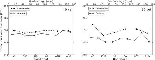
Average mantle transition zone thickness in 1-D (left-hand panel) and 3-D (right-hand panel) wave speed models. In the oceans, the thickness is averaged over every 20-Myr age band and there is no apparent dependence on the age of the sea floor. The average thickness of the mantle transition zone in continental areas is calculated for Asia (AS), Europe (EUR), North America (NA), South America (SA), Africa (AFR) and Australia (AUS). The mantle transition zone is thicker under the continents than under the oceans, especially after crustal and wave speed corrections are applied.
8 COMPARISON WITH PREVIOUS GLOBAL MODELS
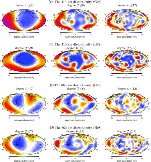
In Fig. 14, we compare the 410- and 660-km discontinuity models in this study with three recent global models imaged based on SS waves and their precursors: Gu et al. (2003), Houser et al. (2008) and Lawrence & Shearer (2008). The four 660-km discontinuity models all show some consistent features. In particular, along subduction zones in the Western Pacific, the 660-km discontinuity is overall deeper than the global average. The mantle transition zone is thicker in the Western Pacific and thinner in the Pacific Ocean. However, large discrepancies exist in the Pacific Ocean. The most extreme disagreement appears to be structures on the 410-km discontinuity maps. For example, the strong depression of the 410-km discontinuity in the Pacific Ocean in Model H08 (Houser et al. 2008) is either absent or much weaker in the other models. The broad uplift of the 660-km discontinuity in the northern Atlantic Ocean in model Model G03 Gu et al. (2003) is weak (absent) in other models. At regional scales, the discrepancies involve reversed polarities in western North America and southeast Asia.

Among all global models, the 410- and 660-km discontinuity depth perturbations obtained from this study agree best with the finite-frequency model published by Lawrence & Shearer (2008) (Model LS08). In Fig. 15, we plot the correlation coefficients between the two models as a function of spherical harmonic degree. The long-wavelength structures in the 660-km discontinuity depth perturbations between the two models are in good agreement, with a positive correlation of ∼0.76 at spherical harmonic degrees l ≤ 4. The correlations are only slightly weaker for the 410-km discontinuity with a correlation coefficient of ∼0.64. Significant discrepancies can be observed in their smaller scale features. For example, the 410-km discontinuity models filtered at spherical harmonic degrees l ≤ 6 starts to show major differences in the Pacific Ocean (Fig. 16), and the correlation coefficient between the two models decreases to ∼0.1 at l = 5−7. At spherical harmonic degree l ≤ 12, the 410-km discontinuity is depressed beneath the Red Sea in our model which is absent in model LS08. A strong negative anomaly in the 410-km discontinuity along the southeast Indian ridge into the southern Atlantic Ocean in model LS08 is absent (much weaker) in our model. Major discrepancies on the 660-km discontinuity include a strong depression beneath the Arabian Plate and the Mediterranean sea in model LS08 and a broad uplift in the Northwest Pacific beneath the old Pacific Plate, which are absent in our model as well as in the other two models (Fig. A2). Overall, the correlations between the new discontinuity model and model LS08 decreases with spherical harmonic degree and there is no apparent correlation between the two models at degree l > 15.
Correlation between discontinuity models in this study and model LS08 (Lawrence & Shearer 2008). The coefficients are plotted as a function of spherical harmonic degree from 1 to 20 for depth perturbations on the 410-km discontinuity, the 660-km discontinuity and the thickness of the mantle transition zone.
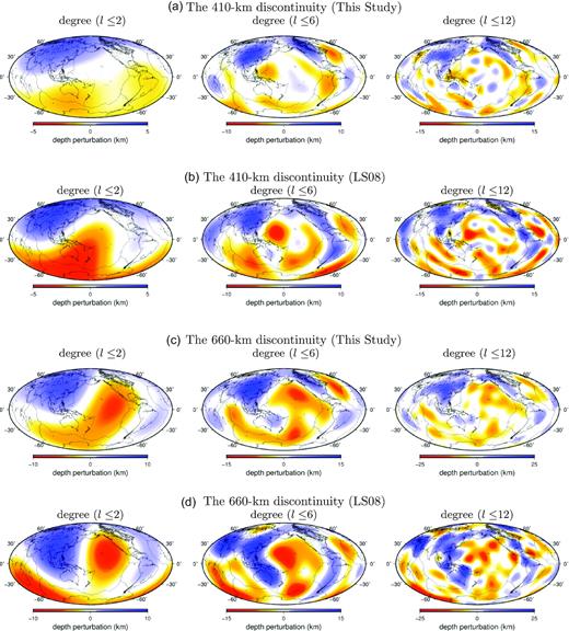
Panel (a) is the 410-km discontinuity model in this study filtered to spherical harmonic l ≤ 2, l ≤ 6 and l ≤ 12. Panel (b) is the same as (a) but for the 410-km discontinuity model from Lawrence & Shearer (2008), panels (c) and (d) are the same as (a) and (b) but for the 660-km discontinuity.
The fact that the general features in the Lawrence & Shearer (2008) model agree better with this study than other ray-theoretical models is somewhat expected as both studies are based on tomographic inversions using finite-frequency sensitivity kernels. The sensitivity kernels in Lawrence & Shearer (2008) were calculated based on ray tracing, which is computationally efficient but the sensitivity kernels do not account for phase interactions and windowing/tapering applied in seismograms. However, it is noteworthy that differences between our finite-frequency models and back-projection models obtained using the exact same data set are less significant than that between the two finite-frequency models. This reflects the importance of using complete finite-frequency sensitivities in data selection and processing. For example, measurements associated with very complex or extreme sensitivity to depth perturbations of the two discontinuities should be excluded.
9 CONCLUSIONS
In this paper, we investigate the finite-frequency effects in imaging the global structure of the 410- and 660-km discontinuities using SS precursors. The finite-frequency SdS–SS traveltime measurements are made using seismograms recorded at GSN stations for earthquakes occurred between 2003 and 2014. The finite-frequency traveltime differences between observed and synthetic seismograms are measured in the frequency domain using a cosine taper. The sensitivity kernels for SS waves and precursors are calculated in the framework of travelling-wave mode coupling, and fully accounts for phase interactions within the measurement window.
The finite-frequency models correlated well with ray-theoretical back-projection models in their large scale structure but the finite-frequency models show much stronger small-scale features when the smoothness (coverage) of the back-projection ray density are comparable to that of the finite-frequency sensitivity density. Crustal and mantle wave speed corrections do not change the general geographic pattern of the SdS–SS traveltime measurements and discontinuity models inverted with and without crustal and mantle corrections are overall well correlated, regardless of the global wave speed models used in making the corrections.
The finite-frequency 660-km discontinuity model is overall positively correlated with wave speed perturbations in the mantle transition zone, indicating a dominant thermal origin for depth perturbations of the 660-km discontinuity. However, a clear correlation between the 410-km discontinuity and seismic wave speed is not observed, which suggests possible non-thermal heterogeneities in the upper mantle transition zone or limited vertical resolution in seismic wave speed tomography. We compare global mantle transition zone discontinuity models obtained from SS precursors and show that our finite-frequency model agrees best with the model of Lawrence & Shearer (2008), which is also a finite-frequency model but with sensitivities calculated based on ray tracing and additional kernel stacking. However, major discrepancies exist between the two models in both oceanic regions and subduction zones, suggesting the significance of wave interference in the calculations of sensitivity kernels as well as the use of finite-frequency sensitivities in data quality control. For example, measurements associated with very complex or extreme sensitivity to discontinuity depth perturbations can be identified in travelling-wave mode coupling and those measurements can be excluded from tomographic inversions.
ACKNOWLEDGEMENTS
We thank Dr Daniel A Frost and an anonymous reviewer for their constructive comments and Editor Ian Bastow for his professional handling of the manuscript. The facilities of the IRIS Data Management System, and specifically the IRIS Data Management Center, were used for access to waveform and metadata required in this study. The authors acknowledge Advanced Research Computing at Virginia Tech for providing computational resources and technical support. This research was supported by the U.S. National Science Foundation under Grants EAR-1737737. All figures were generated using the Generic Mapping Tools (GMT) (Wessel & Smith 1995).
REFERENCES
APPENDIX: MODEL RESOLUTION AND ADDITIONAL MODEL COMPARISON
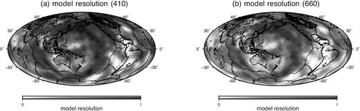
Panels (a) and (b) show the resolution of the finite-frequency 410- and 660-km discontinuity models obtained in this study, plotted in every 4° × 4° grid cell based on diagonal elements of the resolution matrices. In regions where the diagonal elements of the resolution matrix are close to 1, discontinuity depth perturbations are well recovered. The difference between the recovered model and the true model |$\mathbf {x}-\mathbf {x}_{\rm true} = (\mathbf {R}-\mathbf {I}) \mathbf {x}_{\rm true}$| depends on the resolution matrix |$\mathbf {R}$| as well as the earth structure |$\mathbf {x}_{\rm true}$|. For example, in a region where the diagonal element of the resolution matrix is 0.9 and the true depth perturbation is 10 km, the uncertainty due to lack of resolution is about 1 km.
