


SUMMARY
We use the unsupervised and supervised neural network methods together to predict lithology of a gas hydrate reservoir from downhole data in the Krishna–Godavari (KG) offshore basin, India. In this study, we successfully identify the host litho-units of gas hydrate and show its effects in the identification of lithology using neural network techniques, which is not reported earlier. We use well log data acquired at three holes (10A, 03A and 04A) in 2006 during the first expedition of the Indian National Gas Hydrate Program (NGHP-01). Five different logging while drilling data (e.g. density, neutron porosity, gamma ray, resistivity and sonic) are considered for the mapping of lithology and gas hydrate. In the presence of gas hydrate, the resistivity and sonic velocity of the host sediments increase significantly, whereas density, neutron porosity and gamma ray are negligibly affected. Therefore, we calculate resistivity and sonic velocity for water-saturated sediment (without gas hydrate) theoretically to remove the effects of gas hydrate. At first, we apply the seven unsupervised classification methods (i.e. elbow, dendrogram, K-means, 3-D clustering, principal component analysis, Devies–Bouldin index and self-organizing map) to the data with gas hydrate (e.g. observed) and without gas hydrate (i.e. water-saturated/theoretical) to assess the data dimensionality and the number of clusters/litho-units. Each of the unsupervised schemes has its own pros and cons, and may provide different number of cluster/litho-units; sometimes, it is difficult to interpret from only one method. However, all seven methods provide same number of clusters in our study. Then, we apply the supervised classification method (i.e. Bayesian neural networks optimized by hybrid Monte Carlo searching technique) to the training data to refine the defined litho-units and map them with depth. Our approach identifies four types of litho-units and illustrates that the lithology in this area is dominated by clay (∼64 per cent) with some amount of silty clay, silt and minor sand. Gas hydrate is found in clay, silty clay and silt and not in sand. Results also show that, if gas hydrate is not considered as a separate unit, it is distributed as lithology in its hosts (i.e. clay, silty clay and silt). The method is very stable up to ∼15 per cent of random noise added to the data and results are well matched with the analysis of recovered core data. Identified lithologies at three wells correlate very well with seismic section crossing the wells. Very low permeability (<0.1 mD) estimated at three wells also indicates the clay-dominated lithology in our study area.
1 INTRODUCTION
Prediction and classification of subsurface lithology is very important to characterize a reservoir. Various conventional techniques like graphical cross-plotting, core sample analysis, laboratory-based analysis and rock physics modelling are being extensively used for the interpretation of downhole data (Busch et al. 1987; Benaouda et al. 1999; Jana et al. 2015, 2017; Ojha & Maiti 2016; Ojha et al. 2016; Singh et al. 2016) to know the subsurface property of sediments. However, these techniques are semi-automated, purely linear, unable to handle voluminous data (Rogers et al. 1992) and give erroneous results in case of complex and heterogeneous regions. Unavailability of continuous core information due to poor borehole condition is also a problem for these conventional techniques to identify lithology (Baldwin et al. 1990; Benaouda et al. 1999; Helle et al. 2001).
Multivariate statistical analysis, clustering and artificial neural networks (ANNs) can easily overcome the nonlinear problem and predict lithology from downhole data (Baldwin et al. 1990; Rogers et al. 1992; Benaouda et al. 1999; Van der Baan & Jutten 2000; Helle et al. 2001; Chang et al. 2002; Poulton 2002; Aristodemou et al. 2005; Maiti et al. 2007; Maiti & Tiwari 2010a,b; Ojha & Maiti 2016; Karmakar et al. 2018). The unsupervised classification techniques (e.g. elbow, dendrogram, Davies–Bouldin index (DBI), K-means, c-means, density-based spatial clustering, Gaussian clustering, 3-D clustering, self-organizing map (SOM), principal component analysis (PCA), k-nearest neighbour, etc.) are generally used to know the number of classes present in the data in the absence of prior geological information (Banfield & Raftery 1993; Benaouda et al. 1999; Derpanis 2005; Astel et al. 2007; Kriegel et al. 2011; Riedel et al. 2013a,b; Sfidari et al. 2014; Ojha & Maiti 2016; Karmakar et al. 2018). The optimum number of classes obtained from the unsupervised classification techniques are then trained and analysed by using the supervised classification techniques (e.g. ANN, backpropagation (BP), scaled conjugate gradient (SCG), Bayesian neural network (BNN), etc.). Gas hydrates, solid compound of gas (mainly methane) and water are found in the continental margins and permafrost regions, where low-temperature (lower than 300 K) and high-pressure (more than 6 Mpa) conditions along with sufficient amount of gas and water exist. Gas hydrates may be distributed as finely laminated, nodular disseminated and in massive forms depending on the geological condition and types of sediment (Sloan 1990; Kvenvolden & Max 2000). Numerous research works have been carried out in the Krishna–Godavari (KG) offshore basin for delineation, characterization and evaluation of gas hydrate (Cook & Goldberg 2008; Cook et al. 2008; Lee & Collett 2009; Ghosh et al. 2010; Shankar & Riedel 2011; Sain & Gupta 2012; Sain et al. 2012; Wang et al. 2013; Dewangan et al. 2014; Jaiswal et al. 2014; Joshi et al. 2014; Jana et al. 2015, 2017; Ojha et al. 2016). Many researchers have also attempted to classify lithology of gas-hydrate-bearing sediments using ANNs from well logs and seismic data (Ecker et al. 1998; Klose 2006; Matos et al. 2007; Bauer et al.2008, 2015; Collet et al. 2008; Stankiewicz et al. 2010; Riedel et al. 2013a,b), but none of them have addressed the effect of gas hydrate in identifying lithology.
In this paper, we successfully identify the lithology and host lithology of gas hydrate and show the effects of gas hydrate in identifying lithology by applying the unsupervised and supervised classification techniques together. In unsupervised classification, we use elbow, dendrogram, K-means, 3-D clustering, PCA, DBI and SOM. In supervised classification, we use a BNN optimized by hybrid Monte Carlo (HMC) searching technique. The conventional neural network methods are very prone to overfitting (Bhatt & Helle 2002) and do not allow to evaluate uncertainty between input and output variables. It is difficult to choose a regularization parameter without using cross-validation (CV). The BNN method can find the optimum sparsity of a model, which minimizes the overfitting phenomena and maximizes the predictive power of the model. It chooses the model parameters from their probability distribution instead of taking them randomly.
We apply a combined method to the observed data (with gas hydrate) and also to the theoretical data without gas hydrate (water-saturated sediment) to know the effects of gas hydrate in identifying lithology. We also calculate permeability at three holes to know the ability of fluid flow in this area. We compare our predicted lithology with a seismic section passing through these three wells.
2 STUDY AREA AND DATA
Downhole logging data were collected in the KG basin, eastern Indian offshore, under Expedition-01 of Indian National Gas Hydrate Program (NGHP-01) in 2006 (Collett et al. 2008). Drilling and coring were conducted at 10 sites in the KG basin. In this study, we have used the logging while drilling (LWD) data at three holes (NGHP-01-10A, NGHP-01-03A and NGHP-01-04A), which cross a seismic line (Fig. 1). Site NGHP-01-10 is located at 15° 51.86090´ N, 81° 5.07490´ E at a water depth of ∼1038 m, where three holes, NGHP-01-10A, 10B and 10D, were drilled, and LWD data were acquired at hole 10A. Site NGHP-01-03 is located at 15° 53.8919´ N, 81° 53.9678´ E at a water depth of ∼1076 m, where three holes, NGHP-01-03A, 03B and 03C, were drilled, and LWD data were collected at hole 03A. Site NGHP-01-04 is situated at 15° 57.3794´ N, 81° 59.4650´ E at a water depth of ∼1081 m, where only one hole, NGHP-01-04A, was drilled, and LWD data were collected.
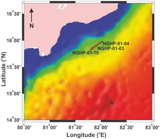
Location map of the study area in the KG offshore basin, eastern continental margin of India. Drill sites (dots) are superimposed on the seismic profile (solid line).
We have used density, neutron porosity, gamma ray, resistivity and sonic logs in our study (Figs 2 –4). Increases in resistivities and P-wave velocities with respect to the water-saturated sediment (Figs 2, 3 and 4d & e) indicate the presence of gas hydrate at all three sites (Collett et al. 2008), which may affect the identification of lithology using neural networks. We have neglected the effects of gas hydrate on density, as the densities of gas hydrate (0.93 g cc−1) and water (1 g cc−1) are almost equal. To remove the effects of gas hydrate, we have calculated resistivity and P-wave velocity for water-saturated sediment (without gas hydrate) using Archie's law (Archie 1942) and the three-phase Biot-type equation (Lee & Collet 2009), respectively. Observed density, neutron porosity, gamma ray, resistivity at bit and P-wave velocity at three holes (NGHP-01-10A, -03A and -04A) are shown by black lines in Figs 2–4, respectively. The bottom simulating reflectors (BSRs) are marked on the log data by the dashed black line. Resistivity and P-wave velocity of water-saturated sediments at three holes are shown by green lines in Figs 2d & e, 3d & e and 4d & e, respectively. We have applied the neural network technique on both data (with and without gas hydrate) separately to know the effects of gas hydrate in the identification of lithology.
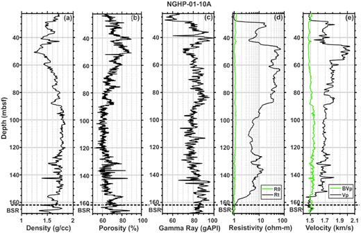
Observed (a) density, (b) neutron porosity, (c) gamma ray, (d) resistivity at bit (Rt, black line) with the background trend (R0, green line) and (e) sonic velocity (Vp, black line) with the background trend (BVp, green line) at hole NGHP-01-10A. The BSR at depth of ∼163 m is shown by the dashed black line.
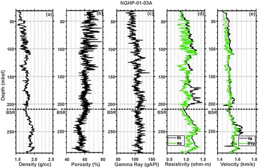
Observed (a) density, (b) neutron porosity, (c) gamma ray, (d) resistivity at bit (Rt, black line) with the background trend (R0, green line) and (e) sonic velocity (Vp, black line) with the background trend (BVp, green line) at hole NGHP-01-03A. The BSR at depth of ∼209 m is shown by the dashed black line.
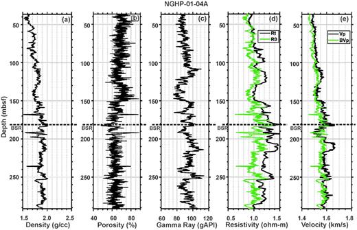
Observed (a) density, (b) neutron porosity, (c) gamma ray, (d) resistivity at bit (Rt, black line) with the background trend (R0, green line) and (e) sonic velocity (Vp, black line) with the background trend (BVp, green line) at hole NGHP-01-04A. The BSR at depth of ∼182 m is shown by the dashed black line.
3 METHODS
For classification of lithology, we have applied unsupervised and supervised classification techniques on both data (e.g. the data with and without gas hydrate). The detailed workflow of the method including unsupervised and supervised schemes is provided in Fig. A1. In unsupervised techniques, seven clustering methods—elbow, dendrogram, DBI, K-means, 3-D clustering, PCA and SOM—have been used to know the optimum number of classes along with specific ranges of the given data. The elbow, dendrogram and DBI methods give the optimum number of classes without visualizing the data. However, the K-means and 3-D clustering provide number of classes as well as their specific range by visualizing the data in 2-D and 3-D maps, respectively. The PCA and SOM give only optimum number of classes by visualizing the data in 2-D and 3-D map. The unsupervised classification determines the number of classes along with lithology, which are not mapped with depth. Training samples are generated using the number of classes along with their optimum ranges obtained from unsupervised classification (K-means and 3-D clustering). Then, the supervised classification technique is applied to the trained samples to refine the defined cluster units and map them with depth. Permeability is estimated based on the Kozney–Carman equation (Kozney 1927; Carman 1937), the Schlumberger–Doll–Research equation (Kenyon et al. 1988) using nuclear magnetic resonance (SDR-NMR) and the clay fraction-derived equation (Yang & Alpin 2010) at three sites. Unsupervised classification techniques and estimation of permeability are briefly described in Appendices A and C, respectively.
3.1 Supervised techniques
In the supervised classification technique, we have used a multilayer perceptron (MLP) configuration (Meier et al. 2007; Ojha & Maiti 2016). The MLP architecture classifies overlapping signal by nonlinear mapping from a set of correct training samples. In the MLP configuration, we have used three layers, where input (log data) and output (lithology) are connected with a hidden layer with synaptic weights.
This technique works in an iterative way describing the functional relationship between input (here well log) and output space/domain (lithology class) from a finite data set (|$Z\ = \ \{ {{x_k},{y_k};k\ = \ 1, \ldots .,N} \}$|) by minimizing the misfit/cost function. The BP algorithm is used to minimize the cost function by adjusting network weights and biases (Rumelhart et al. 1986; Dai & Macbeth 1997; Devilee et al. 1999). Conventionally, weights and biases are generated randomly, which are very prone in overfitting and do not allow estimation of the uncertainty (Bishop 1995; Bhatt & Helle 2002; Khan & Coulibaly 2006). The overfitting problem can be minimized by CV and early stopping techniques (ESTs; Van der Bann & Jutten 2000). In the CV technique, the training samples are split into training, validation and test data sets. Weights are optimized by using the training data set, where cross-validation using the validation data set confirms the overall performance of the network (Van der Bann & Jutten 2000). The EST technique is carried out by updating the network performance on the test data sets in an iterative way, which provides the guidance about how many iterations are required before the network starts overfitting (Prechelt 1998). However, these techniques are not found to be best to overcome the overfitting due to inaccurate generalization capacity of a model (Hippert & Taylor 2010). The BNN method overcomes the overfitting problem better by calculating the probability distribution of the model parameters instead of taking model parameters randomly. The BNN also regularizes the weights and biases to control the noise in data. The BNN provides better results through probabilistic promises on predictions and also generating the distribution of model parameters, which has been learnt from a set of observations. The BNN also helps to calculate the uncertainty present in the output of the network. The detailed mathematical explanation of BNN–HMC is given in Appendix B.
3.2 Estimation of permeability
Permeability is an important petro-physical property that measures material's ability of permitting fluids to pass through it without altering the structure of the medium. Accurate estimation of permeability is very essential for hydrocarbon production, which contributes the knowledge about the production rates and optimizes drainage strategies and also locates good drainage points for well placement in the reservoir (Rubino et al. 2012). For hydrocarbon production, the material is usually sedimentary rock and fluid is oil, gas or water (North 1985; Rubino et al. 2012). Here, we have estimated permeability at these three respective holes by using three different equations: (i) the Kozney–Carman equation (ii) the clay fraction-derived equation and (iii) the SDR-NMR equation, which are described in Appendix C.
4 RESULTS
Seven unsupervised methods have been applied to obtain the number of classes in the data, where all techniques give the same number of classes. Figs 5(a) and (b) show the elbow method, where the sum of the intracluster distances decreases with increasing number of clusters and after a certain point it decreases slowly. These ‘elbow’ points (shown by arrows in Figs 5a and b) are considered as the optimum number of cluster units. We get four classes in the data without gas hydrate (Fig. 5a) and five classes with gas hydrate (Fig. 5b) at hole 10A (solid black line). Three classes are present in the data without gas hydrate (Fig. 5a) and four classes are present in the data with gas hydrate (Fig. 5b) at both holes 03A (dashed black line) and 04A (dotted black line). Figs 5(c) and (d) show the DBI versus the number of clusters, where the lowest DBI values indicate the number of classes present in the data. To know the number of classes present in the data, we have also carried out dendrogram analysis, where the branches occurring at about the same distance indicate the number of classes as shown in Fig. D1 in Appendix D.
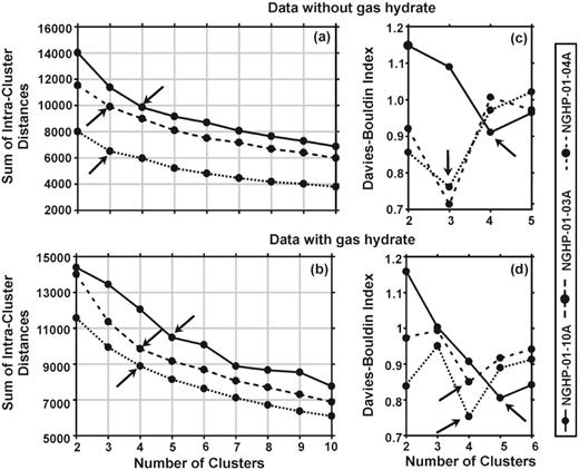
The plot shows the number of clusters versus sum of intracluster distances in (a and b) the elbow method and (c and d) Davies–Bouldin index value versus number of clusters for data (a and c) without gas hydrate and (b and d) with gas hydrate at three holes: NGHP-01-10A (solid), -03A (dashed) and -04A (dotted). Arrows show the first major breaking points as the number of classes present at different holes.
Fig. 6 demonstrates the K-means clustering results between resistivity and gamma ray logs (Figs 6a, e, i, c, g and k) and between velocity and gamma ray logs (Figs 6b, f, j, d, h and l) for data without (left two panels) and with gas hydrate (right two panels) at holes 10A (top panel), 03A (middle panel) and 04A (bottom panel). Stars in Fig. 6 represent the centroids of different clusters, where colours represent different classes along with their range in log measurements. The K-means clustering suggests that four classes (e.g. clay, silty clay, silt and sand) in the data without (Figs 6a and b) and five classes (e.g. clay, silty clay, silt, sand and gas hydrate) with gas hydrate (Figs 6c and d) are present at hole 10A. At holes 03A and 04A, three classes (e.g. clay, silt and sand) in the data without (Figs 6e, f, i and j) and four classes (e.g. clay, silt, sand and gas hydrate) with (Figs 6g, h, k and l) gas hydrate are present. It is noted that in Fig. 6, the gas hydrate has also been identified as a distinctive cluster unit with specific bounds of various well log responses. Mainly clay, silt and sand are present in all three sites, except some silty clay at hole 10A.
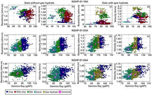
K-means cluster analysis at three holes, NGHP-01-10A (top panel: a–d), -03A (middle panel: e–h) and -04A (bottom panel: i–l), based on the cross-plot between gamma ray and resistivity, and gamma ray and velocity for data without (left two panels: a, b, e, f, i and j) and with (right two panels: c, d, g, h, k and l) gas hydrate. Colours represent various clusters with their respective centroids (stars).
Fig. 7 illustrates the 3-D clustering among porosity, resistivity and gamma ray, and porosity, velocity and gamma ray for the data without (left two panels) and with (right two panels) gas hydrate at three holes. From Fig. 7, it is clearly observed that four litho-units are present at hole 10A in the data without gas hydrate (Figs 7a and b) and five litho-units are present in data with gas hydrate (Figs 7c and d). Similarly, Fig. 7 also reveals three litho-units in data without gas hydrate (Figs 7e, f, i and j) and four litho-units in data with gas hydrate at holes 03A and 04A (Figs 7g, h, k and l). The K-means and 3-D clustering methods provide number of classes present in the data as well as ranges of log response for different classes. The K-means and 3-D clustering illustrate that most of the data points are classified by a definite cluster unit, except some overlapping points at the boundary between two classes (Figs 6 and 7).
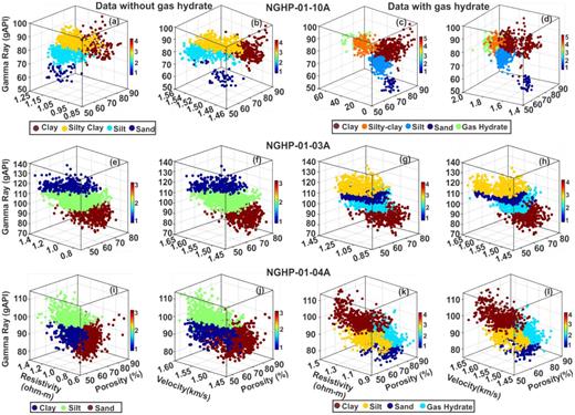
3-D cluster analysis at three holes, NGHP-01-10A (top panel: a–d), -03A (middle panel: e–h) and -04A (bottom panel: i–l), based on the cross plot among porosity, resistivity and gamma ray, and porosity, velocity and gamma ray for data without (left two panels: a, b, e, f, i and j) and with (right two panels: c, d, g, h, k and l) gas hydrate. Various litho-units are represented by different colours.
Next, we perform PCA to know which variables (log measurements) play dominant role in classifying lithology. The PCA has been carried out using five variables (e.g. density, porosity, gamma ray, resistivity and velocity) on both data sets (data with and without gas hydrate) at three holes (Fig. 8). Fig. 8 illustrates the variances of the variables along y-axes against the principal components along x-axes. Fig. 8 suggests that porosity [PC(1)] and gamma ray [PC(2)] logs play a significant role (Figs 8a1, a2, b2, c1, c2, d1, d2, e1, e2, f1 and f2) in classifying lithology at three holes in case of both data (without and with gas hydrate), except at hole 10A, where resistivity [PC(1)] also plays a major role in case of data with gas hydrate (Fig. 8b1), which may be due to the presence of high amount of gas hydrate at this site. In PC(2), porosity log and gamma ray log have a dominant role in the same direction at both holes 03A and 04A (Figs 8c2, d2, e2 and f2) but in opposite direction at hole 10A for both data sets (Figs 8a2 and b2). In PC(3), density and resistivity logs play a dominant role in both data sets at all holes (Figs 8a3 and c3–f3), except at hole 10A, where porosity plays the major role (Fig. 8b3). However, in PC(4) and PC(5) density, velocity and resistivity logs play a leading role in both positive and negative directions for all three holes (Figs 8 a4–f4 and a5–f5).
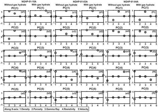
Role of each variable (well log) for classification of the lithology (a–f), where x-axes represent different physical parameters and y-axes represent principal component coefficients (variance). Maximum variance indicates the dominant principal component.
Cross-correlations among the different variables show that at hole 10A, (i) porosity log has positive correlation with gamma ray log (Figs 9a and d) and negative correlation with resistivity and velocity logs in data without gas hydrate (Fig. 9a), whereas porosity log is positively correlated with velocity and resistivity logs in data with gas hydrate (Fig. 9d); (ii) the density log has zero correlation with gamma ray log (Figs 9a and d) and positive correlation with velocity and resistivity logs in data without gas hydrate (Fig. 10a), but negative correlation with velocity and resistivity logs in data with gas hydrate (Fig. 10d) and (iii) the resistivity log correlates positively with velocity log and negatively with gamma ray log in data without gas hydrate (Fig. 9a). Similarly, the cross-correlations at holes 03A and 04A suggest that resistivity log is positively correlated with density, gamma ray and velocity logs but negatively correlated with porosity log in both the data sets (Figs 10 and 11a & d). Porosity log has high negative correlation with density, gamma ray, velocity and resistivity logs at holes 03A and 04A (Figs 10 and 11a & d), whereas gamma ray log has a positive correlation with density, resistivity and velocity logs but negative correlation with porosity log at holes 03A and 04A (Figs 10 and 11a & d). Figs 10 and 11(b) & (e) suggest that 99 per cent variance of both data sets is explained by first two principal components (density and porosity) at holes 03A and 04A. However, at hole 10A, first two principal components (density and porosity) are required for data without gas hydrate (Fig. 9b) and three principal components (density, porosity and resistivity) are required for data with gas hydrate (Fig. 9e) to explain 99 per cent variance of data. Therefore, the multivariable data set can be visualized using only two coordinate axes, except the data with gas hydrate at hole NGHP-01-10A. The PCA-based classifications show four classes (e.g. clay, silty clay, silt and sand) in the data without gas hydrate (Fig. 9c) and five classes (e.g. clay, silty clay, silt, sand and gas hydrate) in the data with gas hydrate of hole 10A (Fig. 9f). However, at holes 03A and 04A, three classes (e.g. clay, silt and sand) are present in data without gas hydrate (Figs 10 and 11c) and four classes (e.g. clay, silt, sand and gas hydrate) are present in data with gas hydrate (Figs 10 and 11f).
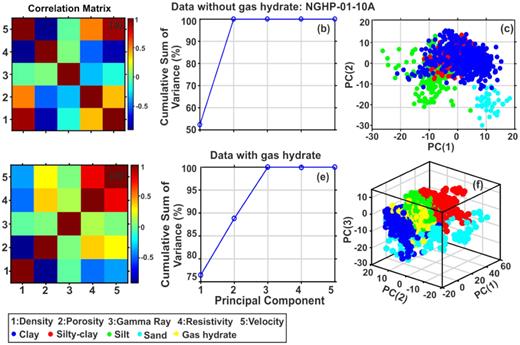
Correlation analysis of variables (well logs) for principal component analysis (PCA) (a and d), cumulative sum of variance of different principal components (b and e) and PCA-based classification (c and f) for the data without (top) and with (bottom) gas hydrate at hole NGHP-01-10A.
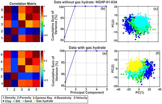
Correlation analysis of variables (well logs) for principal component analysis (PCA) (a and d), cumulative sum of variance of different principal components (b and e) and PCA-based classification (c and f) for the data without (top) and with (bottom) gas hydrate at hole NGHP-01-03A.
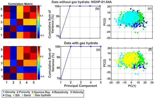
Correlation analysis of variables (well logs) for principal component analysis (PCA) (a and d), cumulative sum of variance of different principal components (b and e) and PCA-based classification (c and f) for the data without (top) and with (bottom) gas hydrate at hole NGHP-01-04A.
Fig. 12 illustrates the SOM-based classification of both data sets. The size of the U-matrices for training the data sets was calculated and their dimensions consist of 400 units for hole 10A and 200 units for holes 03A and 04A. The U-matrices of different holes are presented with different colour codes for three holes (Figs 12a, c, e, g, i and k). The SOM-based results visualize different number of cluster units present in both data. At hole 10A, four cluster units exist in data without gas hydrate and five cluster units exist in data with gas hydrate (Figs 12b and d). Similarly, at holes 03A and 04A, three cluster units are present in data without gas hydrate (Figs 12f and j) and four cluster units are present in data with gas hydrate (Figs 12h and l). Fig. 12 also describes the presence of gas hydrate as a distinct cluster unit in data with gas hydrate at three holes. PCA and SOM methods visualize same number of cluster units in both data sets at three holes.
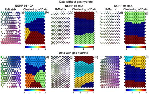
Representation of U-matrix colour coding for data without (a, e and i) and with (c, g and k) gas hydrate and clustering corresponds to K-means clustering for data without (b, f and j) and with (d, h and l) gas hydrate at holes 10A, 03A and 04A.
Table 1 displays the significant range of various downhole logs for generating the samples (inputs and their corresponding output pairs) for BNN–HMC-based supervised classification. We have prepared three different sets of training samples for the initial model: (i) training samples for data without gas hydrate, (ii) training samples for data with gas hydrate, and (iii) training samples for data without considering gas hydrate as a separate litho-unit in observed data (Table 1). These training samples are generated with utmost care and verified using available core sample information. We have prepared more training samples than the number of network's internal variables as suggested by Van der Bann & Jutten (2000) to keep the optimization problem overconstrained.
The significant limits to generate a forward model in neural network training of the data sets at three holes. Here, subscripts W, H and NC denote the data without gas hydrate (i.e. water-saturated sediments), data with gas hydrate (i.e. observed data) and data without considering gas hydrate as a separate litho-unit in observed data, respectively. Holes NGHP-01-10A, -03A and -04A are represented by 10, 3 and 4, respectively. Lithology that is not observed is denoted by NO.
| Lithology/Rock type | Density (g cc−1) | Porosity (%) | Gamma ray (gAPI) | Resistivity (ohm m) | Velocity (km s−1) | Desired output (binary code) |
|---|---|---|---|---|---|---|
| Clay | 1.24–1.6810W | 70–9010W | 70–9910W | 0.85–1.1210W | 1.47–1.5110W | 100010W |
| 1.24–1.610H | 70–9010H | 70–9910H | 4–1810H | 1.5–1.810H | 1000010H | |
| 1.24–1.710NC | 70–9010NC | 70.5–9910NC | 3.7–1810NC | 1.5–1.8110NC | 100010NC | |
| 1.62–2.03W | 46–713W | 108–1393W | 0.8–1.403W | 1.47–1.623W | 1003W | |
| 1.61–2.03H | 47–693H | 114–1393H | 0.96–1.433H | 1.49–1.663H | 10003H | |
| 1.62–2.03NC | 46–713NC | 108–1393NC | 0.96–1.433NC | 1.5–1.673NC | 1003NC | |
| 1.66–2.014W | 50–734W | 93–1144W | 0.82–1.324W | 1.48–1.624W | 1004W | |
| 1.66–2.014H | 50–734H | 94–1144H | 0.96–1.504H | 1.5–1.674H | 10004H | |
| 1.66–2.014NC | 50–734NC | 94–1144NC | 0.96–1.514NC | 1.5–1.684NC | 1004NC | |
| Silty clay | 1.37–1.8110W | 62–8810W | 80–9610W | 0.87–1.1610W | 1.48–1.5110W | 010010W |
| 1.37–1.8110H | 62–8910H | 73–9610H | 1–2010H | 1.44–1.7610H | 0100010H | |
| 1.37–1.8110NC | 62–9010NC | 75–9610NC | 1–20.510NC | 1.44–1.8710NC | 010010NC | |
| NO3W | NO3W | NO3W | NO3W | NO3W | NO3W | |
| NO3H | NO3H | NO3H | NO3H | 1.49–1.663H | NO3H | |
| NO3NC | NO3NC | NO3NC | NO3NC | 1.5–1.673NC | NONC | |
| NO4W | NO4W | NO4W | NO4W | NO4W | NO4W | |
| NO4H | NO4H | NO4H | NO4H | NO4H | NO4H | |
| NO4NC | NO4NC | NO4NC | NO4NC | NO4NC | NO4NC | |
| Silt | 1.48–1.8410W | 54–7010W | 70.5–8710W | 0.96–1.1510W | 1.48–1.5610W | 001010W |
| 1.44–1.7410H | 58–7210H | 70–9210H | 22–4610H | 1.68–1.8810H | 0010010H | |
| 1.46–1.8410NC | 58–7210NC | 70–9310NC | 24–7110NC | 1.68–2.0310NC | 001010NC | |
| 1.55–1.983W | 50–763W | 96–1103W | 0.76–1.363W | 1.46–1.623W | 0103W | |
| 1.56–1.963H | 52–763H | 94–1083H | 0.85–1.43H | 1.46–1.593H | 01003H | |
| 1.55–1.983NC | 50–763NC | 96–1103NC | 0.86–1.43NC | 1.46–1.663NC | 0103NC | |
| 1.54–1.984W | 54–694W | 78–954W | 0.80–1.204W | 1.46–1.614W | 0104W | |
| 1.54–1.984H | 54–68.74H | 78–94.14H | 0.92–1.414H | 1.48–1.634H | 01004H | |
| 1.54–1.984NC | 54–694NC | 78–944NC | 0.92–1.414NC | 1.48–1.624NC | 0104NC | |
| Sand | 1.6–1.7610W | 60–7310W | 54–6910W | 1.04–1.2110W | 1.49–1.5210W | 000110W |
| 1.61–1.7610H | 59–7110H | 54–6610H | 0.9–8.010H | 1.47–1.710H | 0001010H | |
| 1.6–1.7610NC | 60–7310NC | 54–6810NC | 0.9–8.010NC | 1.47–1.710NC | 000110NC | |
| 1.53–1.93W | 53–76.53W | 75–983W | 0.77–1.303W | 1.45–1.583W | 0013W | |
| 1.51–1.93H | 53–773H | 75–953H | 0.84–1.243H | 1.45–1.543H | 00103H | |
| 1.53–1.93NC | 53–773NC | 75–983NC | 0.84–1.283NC | 1.45–1.573NC | 0013NC | |
| 1.56–1.964W | 67–904W | 75–954W | 0.70–1.14W | 1.45–1.584W | 0014W | |
| 1.56–1.964H | 67–904H | 75–954H | 0.88–1.254H | 1.47–1.614H | 00104H | |
| 1.56–1.964NC | 67–904NC | 75–954NC | 0.88–1.264NC | 1.48–1.614NC | 0014NC | |
| Gas hydrate | NO10W | NO10W | NO10W | NO10W | NO10W | NO10W |
| 1.58–1.8510H | 68–9010H | 70–8710H | 40–7110H | 1.8–2.0410H | 0000110H | |
| NC10 | NC10 | NC10 | NC10 | NC10 | NC10 | |
| NO3W | NO3W | NO3W | NO3W | NO3W | NO3W | |
| 1.6–2.033H | 52–743H | 102–1143H | 0.94–1.433H | 1.51–1.673H | 00013H | |
| NC3 | NC3 | NC3 | NC3 | NC3 | NC3 | |
| NO4W | NO4W | NO4W | NO4W | NO4W | NO4W | |
| 1.5–1.964H | 63–874H | 89–1014H | 0.9–1.444H | 1.49–1.654H | 00014H | |
| NC4 | NC4 | NC4 | NC4 | NC4 | NC4 |
The total data sets of training samples are divided using MATLAB-based code (Maiti & Tiwari 2010a,b). At hole 10A, the number of training samples for data (i) without gas hydrate is 420, (ii) with gas hydrate is 508 and (iii) without considering gas hydrate as a separate litho-unit in observed data is 420. At hole 03A, the number of training sample for data (i) without gas hydrate is 472, (ii) with gas hydrate is 560 and (iii) without considering gas hydrate as a separate litho-unit in observed data is 472. At hole 04A, the number of training sample for data (i) without gas hydrate is 516, (ii) with gas hydrate is 620 and (iii) without considering gas hydrate as a separate litho-unit in observed data is 516. The first 50 per cent data series of all three holes (50 per cent of the total data set) is used for training. The remaining 50 per cent data are used for examining the ‘generalization’ capability of the trained network. Here, about 24.85 per cent of the second 50 per cent data is kept for validation and the remaining portion of the data (about 25.14 per cent) is used for testing (Maiti & Tiwari 2010a,b). Next, we have scaled input/target data to ± 1 for smooth mapping. We have performed a number of simulations and calculated the mean square error (MSE) on training, validation and test data sets and taken its average value with hidden layer nodes by varying from 5 to 30 for both the data sets. Figs 13(a)–(c) show that MSEs are decreasing as the number of hidden nodes is increasing on both data sets and we have preferred that number of hidden nodes where the MSE is minimum. To avoid overfitting phenomena, we have kept the hidden layers to be 7 at hole 10A and 9 for holes 03A and 04A for final analysis (Figs 13a–c). However, we note that beyond this number of hidden nodes there is a sudden increase of MSE in both data sets. This work is a sampling-based algorithm where the leapfrog scheme updates the candidate state. The new state is accepted when the threshold value is greater than the Metropolis acceptance probability, which is a random number varying between 0 and 1 decided at each step (Figs 13d–f). The acceptance rate is very important for successful optimization. The acceptance rate is the rate of accepting samples, which is the ratio of the number of unique values in the Markov chain Monte Carlo (MCMC) chain and the total number of values in the MCMC chain. The acceptance probability represents less number of rejected sample for successful optimization. If it is close to 0, then it will give poor convergence, and for 1, all steps will be accepted and the result will be a linear approximation. Here, the acceptance rate is 0.82 for hole 10A and 0.85 for holes 03A and 04A, which is quite satisfactory (Figs 13d–f). In addition, for successful training the following parameters have been used: (i) the number of nodes in the input layer is 5 for both the data sets at three holes, (ii) at hole 10A, the number of nodes in the output layer is 4 for data without considering gas hydrate as a separate litho-unit in observed data and 5 for data with gas hydrate; at holes 03A and 04A, the number of nodes in the output layer is 3 for data without considering gas hydrate as a separate litho-unit in observed data and 4 for data with gas hydrate; (iii) the initial prior hyperparameters values of |$\lambda \ = \ 0.01$| and |$\mu \ = \ 50.0$| are fixed for all data sets; and (vi) step size is 0.002 and total iterations are 300. We have run the sampling phase of MCMC simulations for 300 iterations, where the initial 200 iterations were discarded to ensure that the simulation attains the equilibrium distribution. However, it is sometimes difficult to know when the simulation reaches the equilibrium (Neal 1996). Therefore, we run numerous simulations to ensure the stability of the output results.
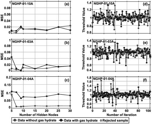
Error analysis with respect to the number of nodes in hidden layer for data without and with gas hydrate (a–c); hybrid Monte Carlo simulations versus number of iterations for without and with gas hydrate (d–f) at holes NGHP-01-10A, -03A and -04A.
The regression analysis provides the slope and intercept values of the best linear regression fit between the output by neural network (y-axis) and the target data (x-axis). The results from this analysis between the target lithology and the output predicted by BNN–HMC suggest that the lithology can be resolved very well with a high positive correlation coefficient at all three holes (Figs 14 –16, respectively), NGHP-01-10A, -03A and -04A. The linear regression analysis shows excellent (∼99 per cent) accuracy for resolving different types of lithology at three holes in the KG basin.

Linear regression analysis between neural network output and target for data (a–d) without and (e–i) with gas hydrate at hole NGHP-01-10A.

Linear regression analysis between neural network output and target for data (a–c) without and (d–g) with gas hydrate at hole NGHP-01-03A.
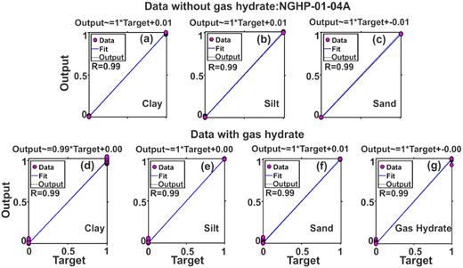
Linear regression analysis between neural network output and target for data (a–c) without and (d–g) with gas hydrate at hole NGHP-01-04A.
Prior to actual BNN application to real well log data, the network's stability has been tested in the presence of different levels of correlated random noise. This is done because, in many geological/geophysical situations, we note some kinds of inherent noise, which dominates the field observations and corrupts the actual signal. The inherent noise that often occurs through errors in well log data is usually caused by washout, caving and deplorable borehole conditions. We have followed the guidance of the random noise analysis (Maiti & Tiwari 2010b). After successful completion of network training, analysis for different levels of random noise has been performed on validation and test data sets. The noise sensitivity analysis of both data sets indicates that the network is stable even if we add up to 15 per cent of correlated random noise to the well log records (Fig. 17).
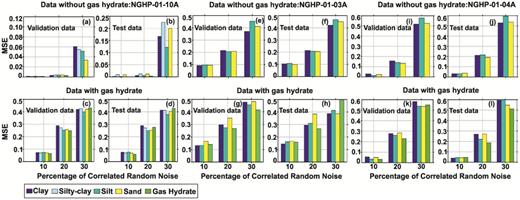
The error analysis of network with different levels of correlated noise added to the validation and test samples for data (a, b, e, f, i and j) without and (c, d, g, h, k and l) with gas hydrate at holes NGHP-01-10A, -03A and -04A, respectively.
The performance of the BNN–HMC model is further tested by the statistical analysis such as standard deviation (SD), root mean squared error (RMSE), reduction error (RE) and index of agreement (IA) (Supporting Information Table S1). The values of IA and RE should be 1.0 for perfect fitting. In this analysis, IA and RE values for the clay, silty clay, silt, sand and gas hydrate of hole 10A have been found to be 0.99 for both the data sets (Supporting Information Table S1). Similar analysis has also been done for holes 03A and 04A, which is available in the Supporting Information. Supporting Information Table S1 provides predictive skill of the model that is able to classify the lithology at three holes in the KG basin.
After successful completion of training, density, porosity, gamma ray, resistivity and velocity log data have been applied to the trained network and the lithology was predicted by the BNN–HMC technique. The output of the network is interpreted as neural-network-based lithological section with depth using BNN–HMC-based modelling from data without and with gas hydrate. The output section of each lithology is displayed in colour matrix (Figs 18a & b, 19a & b and 20a & b). It is noted that along the entire litho-section maximum posterior value is considered as the final lithology model for both the data sets at these holes (Figs 18a & b, 19a & b and 20a & b). The predicted output value close to 1.0 specifies the occurrence of particular lithology with corresponding depth, whereas the value close or equal to 0.0 indicates the absence of particular lithology at that depth. This analysis reveals four types of lithology, that is, clay, silty clay, silt and sand, with depth at three holes in the KG basin (Figs 18a & b, 19a & b and 20a & b, respectively). The lithological section at three holes indicates that it is mainly dominated by clay and silt with a small amount of sand (Figs 18a & b, 19a & b and 20a & b). Moreover, the distribution pattern of lithology remains constant for data without and with gas hydrate. Significantly, it is also identified that the distribution of sand litho-unit is quantitatively high for hole NGHP-01-04A compared to other two holes (Figs 20a and b). The lithology profile at hole 10A is mainly composed of clay, silty clay and silt with minor amount of sand in data both without and with gas hydrate (Figs 18a and b). Similarly, the litho-section at holes 03A and 04A contains higher amount of clay and silt with small amount of sand in data both without and with gas hydrate (Figs 19a & b and 20a & b). Figs 18(b), 19(b) and 20(b) demonstrate that gas hydrate has been modelled and identified from well log data by applying BNN–HMC-based classification technique at three respective holes in the KG basin. From Figs 18(b), 19(b) and 20(b), it is observed that gas hydrate is distributed mainly in clay, silty clay and silt and not in sand at all three holes, respectively. Therefore, it can be concluded that gas hydrate, which is overlapped with lithology containing clay, silty clay and silt, can be identified by the BNN–HMC-based classification technique.
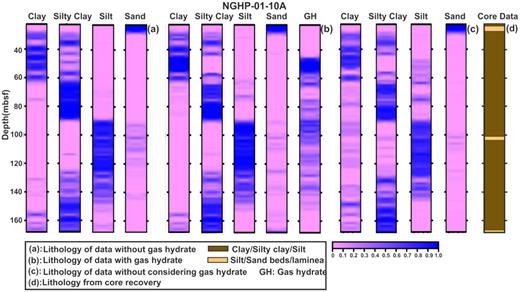
Predicted lithology with depth using the BNN–HMC technique for (a) data without gas hydrate, (b) data with gas hydrate and (c) observed data without considering gas hydrate as a separate litho-unit in the observed data at hole NGHP-01-10A. (d) Lithology obtained from recovered core data.
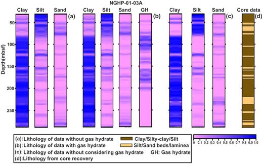
Predicted lithology with depth using the BNN–HMC technique for (a) data without gas hydrate, (b) data with gas hydrate and (c) observed data without considering gas hydrate as a separate litho-unit in the observed data at hole NGHP-01-03A. (d) Lithology obtained from recovered core data.
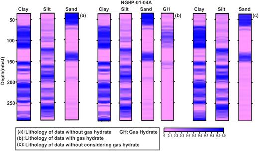
Predicted lithology with depth using the BNN–HMC technique for (a) data without gas hydrate, (b) data with gas hydrate, and (c) observed data without considering gas hydrate as a separate litho-unit in the observed data at hole NGHP-01-04A.
We have repeated the same analysis for data without considering gas hydrate as a separate litho-unit in observed data and tried to interpret the effects of gas hydrate in identifying lithology at all three holes (Figs 18c, 19c and 20c, respectively). This analysis shows that the distribution pattern of lithology has been changed at all three holes (Figs 18c, 19c and 20c) when gas hydrate is not considered as separate litho-unit in observed data. However, we observe that the distributions of lithology have been reformed for clay, silty clay and silt (Figs 18c, 19c and 20c) and not reformed for sand (Figs 18c, 19c and 20c) as clay, silty clay and silt are the hosts of gas hydrate.
The calculated permeability has been plotted with corresponding depth and shown along with gas hydrate saturation obtained from resistivity log and pressure core along with the lithology at all three holes in the KG basin in Fig. 21. Permeability has been calculated to know the drainage properties at three holes using the Kozney–Carman relation, the SDR-NMR-derived relation, and the clay fraction-derived relation for data with gas hydrate (Figs 21g–i). The permeability mainly varies from 10−22 to 10−19 m2 at hole 10A, 10−21 to 10−18 m2 at holes 03A and 04A with depth, except at some depth points, where permeability shows higher values due to the presence of sand/silt (Figs 21g–i). Gas hydrate saturation is derived from resistivity log using Archie's constants |$a\ = \ 3.2$|, |$m\ = \ 0.5$|, and |$n\ = \ 6$| (Jana et al. 2017) for hole 10A; |$a\ = \ 2.3$|, |$m\ = \ 1.7$|, and |$n\ = \ 2$| for hole 03A; and |$a\ = \ 2.5$|, |$m\ = \ 1.5$|, and |$n\ = \ 2$| for hole 04A. Maximum gas hydrate saturations of three holes are found to be about 0.55, 0.18 and 0.22 at holes 10A, 03A and 04A, respectively. The details of deriving Archie's constants and hydrate saturation are described in Appendix E.
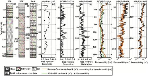
Predicted lithology with depth at three holes (a–c). Gas hydrate saturation derived from resistivity log and direct gas hydrate saturation estimated from pressure cores at holes (d) NGHP-01-10A, (e) -03A and (f) -04A. Estimation of permeability for data with gas hydrate at holes (g) NGHP-01-10A, (h) NGHP-01-03A and (i) NGHP-01-04A. BSRs are marked with the dashed black line at three holes.
Ultimately, a correlation between classified lithology predicted from well log data using the BNN–HMC-based classification technique and the seismic section has been shown in Fig. 22. All major horizons and layers in the seismic section correlate very well with the predicted lithologies/boundaries at three holes.
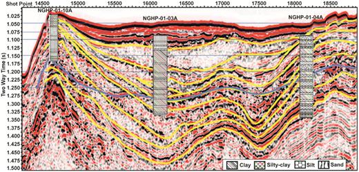
Correlation of predicted lithology with seismic litho-facies. The blue line denotes the BSR, whereas yellow lines indicate various boundaries of sedimentary layers.
5 DISCUSSION
We have used two types of data: data without (theoretical) and with gas hydrate (observed). Calculations of resistivity and sonic velocity for water-saturated sediments (without gas hydrate) are described in Appendix E. Seven unsupervised techniques have been applied to confirm and validate the number of clusters present in two types of data. All seven unsupervised techniques provide same number of clusters in both data sets (data without and with gas hydrate) at three holes. However, each of these methods has some drawbacks and sometimes may show different number of cluster/litho-units or may not be clear to interpret. For example, the elbow method measures only global cluster units, so in case of complex area and in the presence of any lithology with thin layer, it is very hard to find out the first major breaking point. The DBI method provides the best quality of partition in terms of estimating optimum number of clusters in the given data. However, sometimes, it is unable to capture multidimensionality of the data (Thomas et al. 2014). The dendrogram analysis provides number of classes without any prior information, but it has time complexity to handle voluminous data and most of the time it is affected by outlier branch. The K-means, 3-D clustering, PCA and SOM are very effective methods to visualize as well as cluster the data at the same time. The K-means and 3-D clustering among the seven unsupervised methods used here provide the range of values of various well log measurements for different classes/lithologies. These ranges of values of well log measurements play a significant role in training the input data in supervised classification to predict lithology with depth. The K-means and 3-D clustering are easy to implement and can handle voluminous data. The 3-D clustering technique provides additional confidence in classification of data using three variables. However, the K-means and 3-D clustering depend on prior information about the number of clusters. Here, we have taken predefined number of clusters obtained from elbow, Davies–Bouldin and dendrogram methods. The PCA reduces the number of variables (components) in the given data sets and tells how many components (with highest variance) are sufficient to classify the lithology. The correlation matrix in PCA analysis provides the information about dependence between two variables (components), where positively correlated variables are highly dependent on each other and cannot be used to classify lithology. The number of classes determined from the unsupervised classification is so good that it yields 99 per cent correlation coefficients between target and output in supervised classification. The HMC search technique used here samples the model parameters from network output in a faster way with high acceptance probability than the method used by Riedel et al. (2013b). The error in predicting lithology that may arise due to overlapping of data points among various classes has been taken care initially by generating training samples in an iterative manner, which is overcome later by the BNN-HMC searching technique. During training of samples, the acceptance rate is more than 0.8 at all sites, which gives very good convergence and successful optimization of BNN. The linear regression analysis between target and output of network is ∼99 per cent in our data, which is very good to resolve the classification of lithology at three holes. However, it is sensitive to outlier and subject to overfitting problem. Then, regression begins to model the noise present in the data, rather than model relationship between target and output of the network. This problem can be handled by training the network with proper training samples and calculating probability distribution of model parameters accurately. The network is quite stable up to noise level of 15 per cent in the data, which indicates healthiness of network performance. More than 15 per cent of noise in the data makes the network unstable and reduces the performance. We have calculated the average standard deviation error at the network output by BNN–HMC at three sites to check how gas hydrate leads towards error in lithology prediction. The uncertainty values of predicting lithology at three holes are found to be of the order of about ± 14 per cent, which is quite satisfactory. To examine the authenticity of this classification, we have cross-checked few samples manually by the trained network and the results are presented in Table 2. It is found that the prediction from trained network output is consistent with a geological interpretation based on the well log values and their parametrization (Table 1). Hence, the HMC-based BNN algorithm combined with seven unsupervised techniques, regression analysis, statistical analysis and uncertainty analysis provides confidence about the results in identifying lithology, distribution of gas hydrates and its effects on lithology. The final results show the presence of four lithologies (e.g. clay, silty clay, silt and sand) at hole 10A (Figs 18a–c) and three lithologies (e.g. clay, silt and sand) at holes 03A and 04A (Figs 19a–c and 20a–c, respectively). We found an extra lithology of silty clay at hole 10A. This work clearly indicates that if we do not consider gas hydrate as a separate unit, the prediction of lithology will be erroneous. Less amount of gas hydrate observed at sites 03A and 04A has less effects in predicting lithology. However, at site 10A, higher amount of gas hydrate has more effects in predicting lithology. The predicted lithology matches well with lithology derived from recovered cores (Figs 18 and 19) at sites 10A and 03A. However, at site 04A, there is no recovery of core samples. According to the NGHP-01 report (Collett et al. 2008), at site 10A, gas hydrate exists in mainly clay as solid nodules, high angle and subhorizontal veins as fracture fill, and also disseminated in pores. Although some minor fractures are observed, gas hydrates are distributed in silt and sand layers as disseminated within sediments at sites 03A and 04A, which correlate with our predicted lithology.
Classification of real data taken from different borehole sites in the KG basin and comparison between desired output and actual output from network at different depths. Here, subscripts ‘a’, ‘b’ and ‘c’ in the numerical denote data without gas hydrate, data with gas hydrate and data without knowing gas hydrate at hole KG-10A. Similarly, subscripts ‘m’, ‘n’ and ‘p’ and ‘g’, ‘h’ and ‘k’ in the numerical values denote the same for holes KG-03A and KG-04A, respectively.
| Borehole sites | Depth (mbsf) | Density (g cc−1) | Porosity (%) | Gamma Ray (gAPI) | Resistivity (ohm m) | Velocity (km s−1) | Desired Output (binary code) | Actual output from network |
|---|---|---|---|---|---|---|---|---|
| KG-10a | 29.235 | 1.463 | 73.922 | 71.875 | 1.099 | 1.473 | 1 0 0 0 | 1.015 0.003 0.00 0.017 |
| KG-10b | 11.679 | 1.736 | 1 0 0 0 0 | 1.006 0.001 0.010 0.002 0.00 | ||||
| KG-10c | 11.679 | 1.736 | 1 0 0 0 | 0.832 0.00 0.140 0.028 | ||||
| KG-10a | 83.337 | 1.706 | 63.6376 | 90.8213 | 1.132 | 1.510 | 0 1 0 0 | 0.003 0.998 0.018 0.000 |
| KG-10b | 29.376 | 1.772 | 0 1 0 0 0 | 0.003 1.010 0.0000.007 0.825 | ||||
| KG-10c | 29.376 | 1.772 | 0 1 0 0 | 0.004 1.007 0.001 0.000 | ||||
| KG-10a | 165.938 | 1.342 | 88.101 | 87.747 | 0.867 | 1.477 | 1 0 0 0 | 0.997 0.003 0.000 0.002 |
| KG-10b | 0.993 | 1.509 | 1 0 0 0 | 1.008 0.001 0.010 0.0 0.008 | ||||
| KG-10c | 0.993 | 1.509 | 1 0 0 0 | 0.995 0.000 0.013 0.016 | ||||
| KG-03m | 47.008 | 1.622 | 68.894 | 86.513 | 0.687 | 1.465 | 0 1 0 | 0.00 0.964 0.022 |
| KG-03n | 0.991 | 1.497 | 0 1 0 0 | 0.000 1.004 0.000 0.178 | ||||
| KG-03p | 0.991 | 1.497 | 0 1 0 | 0.000 1.005 0.004 | ||||
| KG-03m | 141.496 | 1.788 | 60.842 | 109.288 | 0.755 | 1.515 | 1 0 0 | 0.983 0.000 0.023 |
| KG-03n | 1.070 | 1.514 | 1 0 0 0 | 0.590 0.010 0.000 0.411 | ||||
| KG-03p | 1.070 | 1.514 | 1 0 0 | 1.000 0.000 0.000 | ||||
| KG-03m | 273.322 | 1.882 | 55.506 | 99.309 | 0.750 | 1.568 | 1 0 0 | 0.847 0.000 0.162 |
| KG-03n | 1.235 | 1.566 | 1 0 0 0 | 0.855 0.040 0.136 0.00 | ||||
| KG-03p | 1.235 | 1.566 | 1 0 0 | 0.694 0.000 0.315 | ||||
| KG-04g | 42.126 | 1.549 | 76.222 | 84.395 | 0.793 | 1.453 | 0 0 1 | 0.006 0.003 0.993 |
| KG-04h | 0.908 | 1.487 | 0 0 1 0 | 0.000 0.003 1.010 0.000 | ||||
| KG-04k | 0.908 | 1.487 | 0 0 1 | 0.000 0.000 1.000 | ||||
| KG-04g | 155.664 | 1.903 | 58.293 | 100.477 | 1.142 | 1.555 | 1 0 0 | 1.004 0.012 0.000 |
| KG-04h | 1.236 | 1.570 | 1 0 0 0 | 0.961 0.012 0.004 0.000 | ||||
| KG-04k | 1.236 | 1.570 | 1 0 0 | 1.008 0.000 0.000 | ||||
| KG-04g | 267.983 | 1.927 | 64.135 | 90.520 | 1.051 | 1.584 | 0 1 0 | 0.005 1.010 0.000 |
| KG-04h | 1.208 | 1.591 | 0 1 0 0 | 0.000 0.928 0.012 0.000 | ||||
| KG-04k | 1.208 | 1.591 | 0 1 0 | 0.000 1.012 0.000 |
The permeability required for gas to flow is about |${10^{ - 19}}$| to |${10^{ - 12}}\,{\mathrm{ m}^2}$|. Here, the calculated permeability varies from |${10^{ - 22}}$| to |${10^{ - 19}}\,{\mathrm{ m}^2}$|, which is lower than the permeability required for the gas to flow. This is due to the presence of high amount of clay-bearing sediments at three respective holes in the KG basin. At hole 10A, gas hydrate saturation varies from 0.4 to 0.5 in the depth interval 27–90 m, where lithology is dominated by impermeable clay-bearing sediments with permeability varying from |${10^{ - 22}}$| to |${10^{ - 20}}\,{\mathrm{ m}^2}$|, which may lead to some difficulty in future gas hydrate production (Figs 21a, d and g). However, for depth interval 90–160 m, moderately high permeability has been estimated but less gas hydrate saturation (0.1 to 0.38) is observed, which does not indicate any possibility in gas hydrate production (Figs 21a, d & g). Likewise, at hole 03A and 04A, comparatively high value of gas hydrate saturation (i.e. 0.1 to 0.2) is found with depths, whereas low permeability (i.e. |${10^{ - 21}}$| to |${10^{ - 19}}\,{\mathrm{ m}^2}$|) may cause some trouble in gas hydrate production (Figs 21e, f, h and i).
6 CONCLUSIONS
The BNN-HMC along with multivariate data analysis (K-means, dendrogram, 3-D cluster data analysis, PCA, SOM) is successfully employed to the well log data at three holes for the classification of rock-type/litho-type successions in the KG basin, eastern Indian offshore. Seven unsupervised classification techniques successfully determine the number of lithologies and also detect the presence of gas hydrate as a unique cluster at all three holes. The HMC-based BNN technique is very efficient and cost-effective to interpret a large amount of data. The BNN–HMC technique maps various litho-units and gas hydrate with depth with 99 per cent correlation between output and the target. Our results reveal that the study area is dominated by clay and silt with minor amount of silty clay (at hole 10A) and sand. This supervised technique is very robust in the presence of about 15 per cent noise in the data. The combined approach of unsupervised and supervised classification techniques is found to be very effective to detect and delineate gas hydrate distribution. Gas hydrate is found to be distributed mainly in clay, silty clay and silt, not in sand. Our results clearly illustrate that if gas hydrate is not considered as a separate unit, it will be distributed as a lithology in its hosts and identification of lithology will be erroneous. The distribution of permeability along with gas hydrate saturation and litho-section helps to recognize the permeable and impermeable layers present at three holes in the KG basin. The estimated permeability is very low (|${10^{ - 22}}$| to |${10^{ - 19}}\,{\mathrm{ m}^2}$|) mainly due to the presence of clay. A good correlation observed between the seismic section and neural network-based lithology section provides an excellent overview about the lithology distribution in the KG offshore basin. This approach is found to be very useful than any other techniques for the identification of lithology in a gas hydrate reservoir.
SUPPORTING INFORMATION
Table S1. Statistical analysis of training, validation and test data. Here, subscripts W and H denote the data without gas hydrate (i.e. water-saturated/theoretical) and the data with gas hydrate (i.e. observed ), respectively, where holes NGHP-10A, -03A and -04A are represented by 10, 03 and 04, respectively. RMSE is the root mean squared error, RE is the reduction error and IA is the index of agreement. Training data are represented by tr, validation data are represented by val and test data are represented by tst.
Please note: Oxford University Press is not responsible for the content or functionality of any supporting materials supplied by the authors. Any queries (other than missing material) should be directed to the corresponding author for the paper.
ACKNOWLEDGEMENTS
We are thankful to the Director, CSIR-NGRI, for giving permission to publish this work and providing all facilities to carry out research work. AS thanks the Science &
Engineering Research Board, a statutory body of Department of Science & Technology (DST), Government of India, for providing her with the financial support to carry out the post-doctoral research work through the SERB-NPDF fellowship (PDF/2017/001981). The Directorate General Hydrocarbons and the Ministry of Earth Sciences, Delhi, are acknowledged for providing financial support and data. We are thankful to reviewers for their suggestions and comments to improve the manuscript.
REFERENCES
APPENDIX A: FLOWCHART
A1 Elbow method
The elbow method gives the optimal number of clusters present in data by observing the first major break (like the elbow point) in the plot of the sum of intracluster distances versus the number of clusters. These optimum numbers of cluster are taken as input in cluster analysis.
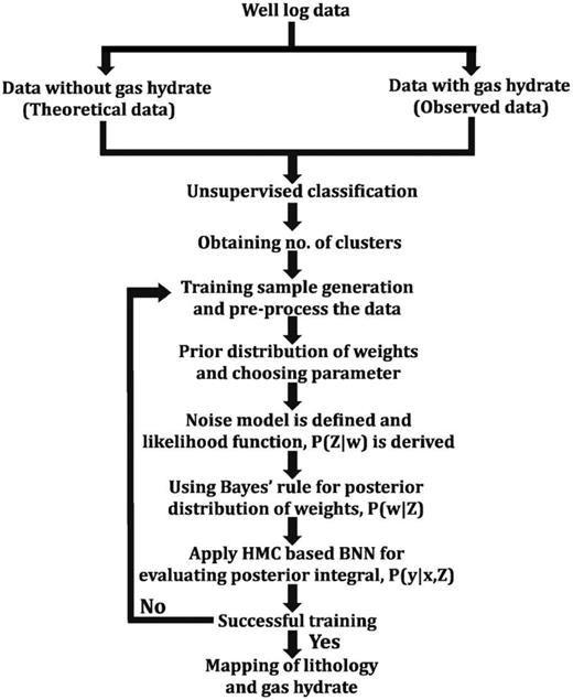
Details of the methods used to predict lithology.
A2 Davies–Bouldin index
A3 Dendrogram analysis
The dendrogram analysis is a hierarchical clustering technique in which the similarity and dissimilarity are measured between the paired samples in an iterative way. Here, we have used Ward's method (Ward 1963). The dendrogram starts by considering each element as a distinct cluster and successively merges them in a larger cluster by minimizing the distance within and maximizing the distance between clusters (Murtagh 1983; Ojha & Maiti 2016; Karmakar et al. 2018). The optimum numbers of clusters determined from the dendrogram analysis are taken as input in cluster analysis.
A4 K-means clustering
A5 3-D clustering
This is a hierarchical clustering technique, which creates clustering of data using Ward's linkage method and visualizes the clusters in a 3-D scatter plot by calculating minimum variance (Ward 1963). Ward suggests a criterion for choosing a pair of clusters based on the optimal value of an objective function, which is computed using squared Euclidean distance between two points. In this algorithm, cluster data return the cluster indices for each observation of the data by minimizing the objective function between two points.
A6 Principal component analysis
The PCA detects the linear dependences between variables and replaces groups of correlated variables by new uncorrelated variables (Jolliffe 1972). Therefore, PCA reduces the dimension of data by dropping the axis that contributes less. Number of data sets (e.g. density, neutron porosity, gamma ray, resistivity and sonic) is the number of principal components. In general, two principal components, PC(1) and PC(2), have greatest variance and can classify lithology. It is important to retain those PCs that have eigenvalues greater than 0.7 to classify lithology better (Jolliffe 1972).
A7 Self-organizing map
After mapping the BMU unit by the centre of the reference vector, the distance between a unit and its neighbour is updated by nearest-neighbour rule (Du 2010). The BMUs are grouped into a unified distance matrix (U-matrix) and presented with different colours for different lithologies by using the K-means clustering more efficiently (Vesanto et al. 1999). The SOM-based classification has been executed using a free Kohonen toolbox (SOM Toolbox 2.0) (Vesanto et al. 1999; Vesanto & Alhoniemi 2000) in MATLAB.
APPENDIX B
B1 Bayesian neural network
B2 Hybrid Monte Carlo technique
APPENDIX C
C1 Kozney–Carman equation
C2 Clay fraction-derived permeability
C3 SDR-NMR equation
APPENDIX D
D1 Clustering using dendrogram analysis
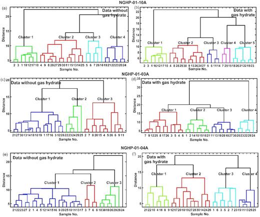
Dendrogram-based clustering at three holes for the data without gas hydrate (a, c and e) and for the data with gas hydrate (b, d and f) at three holes. Branches occurring at about same distance represent the number of classes present in the data.
APPENDIX E
E1 Calculation of resistivity for water-saturated sediment
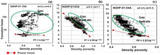
Cross-plot of formation factor versus density-derived porosity for holes (a) NGHP-01-10A, (b) -03A and (c) -04A. The dotted lines show the formation factor versus porosity trend for water-bearing sediments.
