


SUMMARY
It has been increasingly popular to use shallow-seismic full-waveform inversion (FWI) to reconstruct near-surface structures. Conventional FWI tries to resolve the earth model by minimizing the difference between observed and synthetic seismic data using a certain criterion (conventionally, l2-norm of waveform difference). In this paper, we propose a multi-objective waveform inversion (MOWI) in which the similarity of data is quantified and minimized using multiple criteria simultaneously. By doing so, we expand the dimensionality of objective space as well as the mapping from data space to objective space, which provides MOWI higher freedom in exploring the model space compared to single-objective FWI. We combine three different scalar-valued objective functions into a vector-valued multi-objective function which measures the similarity of the waveform, the waveform envelope, and the amplitude spectra of the data, respectively. This multi-objective function takes not only trace-based waveform and wave packet similarity but also the dispersion characteristics of surface waves into account. Furthermore, the uncertainty in the inversion result could be estimated and analysed quantitatively by the variance of the optimal models. We propose a modified ϵ-constraint algorithm to solve the multi-objective optimization problem. Two synthetic examples are used to show the advantages of using MOWI compared to single-objective FWI. We also test the efficiency of MOWI by using two synthetic shallow-seismic examples, which confirm that MOWI can converge to a better result compared to the conventional single-objective FWI.
1 INTRODUCTION
The reconstruction of the shallow subsurface model is of fundamental interest for near-surface geophysics. Conventional shallow-seismic methods, including the first-arrival traveltime tomography and surface-wave phase-velocity inversion, have been proven as efficient ways to reconstruct near-surface structures (Socco et al. 2010; Xia 2014). However, they only use a part of the information contained in seismic data and, thus, have relatively low resolution and accuracy when encountering heterogeneous models. Full-waveform inversion (FWI), which was proposed in the 1980s (Tarantola 1984), reconstructs the subsurface model by fitting the observed waveform directly. It has the ability to reconstruct heterogeneous models by fully exploiting the waveform information and has become increasingly popular in recent years due to the rapid increase in computational power (Virieux & Operto 2009).
Due to the existence of a free surface, surface waves usually dominate the shallow-seismic wavefield, which makes the acoustic approximation no longer valid in shallow-seismic FWI and also increases the ill-posedness of the inverse problem (Gélis et al. 2007; Brossier et al. 2009). Synthetic studies (Romdhane et al. 2011; Nuber et al. 2017) have shown that shallow-seismic FWI, either in the time domain or the frequency domain, is promising in quantitatively imaging the shallow subsurface structures. The applicability of shallow-seismic FWI to reconstruct laterally heterogeneous models with high resolution has been proven recently by real-world applications (Pan et al. 2016; Dokter et al. 2017; Groos et al. 2017; Smith et al. 2019). Due to a relatively high non-linearity and ill-posedness in shallow-seismic FWI, the inversion can be easily trapped in local minima, especially when a poor initial model is provided. Two efficient ways to reduce the ill-posedness of FWI are the smart design of an objective function (e.g. Yang & Engquist 2017; Métivier et al. 2018) and the extension of the search space (e.g. van Leeuwen & Herrmann 2013; Huang et al. 2018). Based on the modification of objective function, two practical approaches that reduce the ill-posedness of shallow-seismic FWI are the windowed-spectrum waveform inversion (Pérez Solano et al. 2014) and the envelope-based waveform inversion (Yuan et al. 2015; Borisov et al. 2017).
FWI usually uses one criterion (one scalar) to measure the data similarity. Since different scalar objective function has its unique features in FWI (e.g. l2 waveform difference has the ‘optimal’ resolution but narrow global minimum width, l2 envelope difference has wider global minimum width but loses polarity information; Pladys et al. 2017), it appears promising to jointly use multiple objective functions to exploit their advantages. One direct way is to sequentially use different objective functions according to their levels of ill-posedness (Pérez Solano et al. 2014; Borisov et al. 2017; Pan et al. 2019). Another approach is to use a more well-posed objective function as an auxiliary function to guide the conventional least-squares functional towards the global minimum (Bharadwaj et al. 2013, 2016).
Due to a huge number of model parameters, the uncertainty estimation in FWI is computationally expensive and is, therefore, usually simplified as a qualitative evaluation of the best-fitting model. This evaluation could be done by checking the flatness of common-image gathers (Plessix et al. 2012), looking at the consistency of source time functions in different shot gathers (Gassner et al. 2019), comparison to migrated images (Operto et al. 2015), or checking the structural similarity with non-seismic results (Wittkamp et al. 2018). Common approaches to perform uncertainty estimation are based on Bayesian inference framework (e.g. Tarantola 2005; Bui-Thanh et al. 2013; Zhu et al. 2016; Fang et al. 2018). They require a good sampling of the model space to approximate posterior, which is usually prohibitively expensive. The utilization of Hessian or inverse Hessian (Fichtner & Trampert 2011; Fichtner & van Leeuwen 2015; Pan et al. 2018) provides a more efficient way to estimate posterior covariance. Besides, the uncertainty estimation can also be done by using square-root variable metric (Liu et al. 2019) and ensemble transform Kalman filter (Thurin et al. 2019). The Bayesian inverse problems (Tarantola 2005) correspond to a scalar-valued optimization problem in the deterministic case. In contrast to that, Shigapov (2019) proposed a parametric probabilistic framework which can be reduced to a multi-objective optimization problem in the deterministic case. He showed with synthetic and real ocean-bottom-cable data that the Pareto optima of the multi-objective problem can be used for uncertainty quantification.
In this paper, we propose a multi-objective waveform inversion (MOWI) of shallow-seismic data. The vector-valued multi-objective function consists of three different single objective functions, which describe the discrepancies between the observed and synthetic waveforms as well as their waveform envelopes in the space–time (x–t) domain, and between their amplitude spectra in the frequency–wavenumber (f–k) domain, respectively. By minimizing the vector-valued multi-objective function, we expand the dimensionality of objective space in the inverse problem. We propose a modified ϵ-constraint method as the optimization algorithm and obtain a set of optimal solutions (models) by evaluating the non-dominance of all solutions. By using the variance of non-dominated solutions, we quantitatively estimate the uncertainty of the inverted model parameters. Two numerical examples and two synthetic inversion tests are used to demonstrate the advantages of using MOWI.
2 METHODOLOGY
2.1 Multi-objective function
Unlike conventional multi-objective geophysical inverse problems in which the vector-valued objective function is composed of the similarity of multiple data types (Heyburn & Fox 2010), our vector-valued objective function |$\boldsymbol{\Phi }{({\bf m})}$| uses multiple measurements of data similarity simultaneously. ϕ1 and ϕ2 describe the discrepancy of the waveforms and the waveform envelopes in the x–t domain, respectively, and ϕ3 describes the discrepancy of the amplitude spectra in the f–k domain. ϕ1 provides an ‘optimal’ resolution in the result (Pladys et al. 2017). ϕ2 is sensitive to the group velocity and the amplitude of surface wave, and provide low non-linearity and convexity to the inverse problem. Unlike ϕ1 and ϕ2 which are trace-based, ϕ3 is a shot-gather-based measurement that also considers the spatial change in the data. Besides, ϕ3 takes one of the most important characteristics of surface wave, dispersion, into account. Thus, the multi-objective function describes the data similarity in a more comprehensive way compared to the single-objective function. MOWI expands the objective space (dimensionality) in the inverse problem, which provides higher freedom in searching and evaluating solutions in the model space. This is because MOWI could use multiple misfit and gradient information from all single-objective functions, thus, is able to avoid, or to jump out of, the local minima which only exist in individual single-objective functions (Bharadwaj et al. 2013).
2.2 Optimization algorithm
It can be seen in eq. (8) that the larger the ϵ value is, the weaker the constraints are adopted. MOWI would become a sequential inversion of multiple objective functions in which any worsening of the constrained misfits is allowed when ϵ approaches infinity. An ϵ value of 1.1 means that worsening no greater than 10 per cent in the constrained objective functions compared to the last iteration is tolerated. We allow a certain worsening so that MOWI is able to jump out of a local minimum which only exists in one or two of the single-objective functions. The choice of ϵ value depends on the consistency of the multiple objective functions, and the less consistent they are, the higher the ϵ value should be adopted.
We choose to firstly minimize ϕ3, then ϕ2 and ϕ1, respectively, in the modified ϵ-constraint method. This is because the f–k spectrum waveform inversion (SWI, ϕ3) and the envelope waveform inversion (EWI, ϕ2) are more convex than the conventional least-squares FWI (ϕ1) (Pan et al. 2019). Furthermore, this sequence avoids frequently jumping between different domains in the data space (i.e. x–t domain and f–k domain) during the inversion. Besides the constraint criterion, we also use another criterion (switching criterion) to move to another single-objective function in the modified ϵ-constraint method: (I) the current objective function does not decrease or (II) the current objective value has been reduced to a certain level (e.g. a factor of 10 in our synthetic examples). These criteria provide the diversity of solution paths. The inversion will move to the next objective function when the constraint criterion or the switching criterion is reached. The inversion will stop when all three single-objective functions diverge consecutively or the maximal iteration number is reached.
2.3 Optimal solution and uncertainty
Unlike the single-objective inverse problem in which there is always a solution that gives the lowest misfit value, we usually obtain a set of optimal solutions in a multi-objective inverse problem. These optimal solutions are found using the concept of non-dominance.
3 NUMERICAL EXAMPLES
3.1 Shapes of objective functions in a consistent case
We use a simple heterogeneous model (Fig. 1) to test the shapes of three objective functions. The true model has a layered background in which the S-wave velocities of each layer are 200, 400 and 600 m s−1, respectively. The thicknesses of the first two layers are 3 and 5 m, and the P-wave velocity is set as three times of S-wave velocity. A constant density of 2000 kg m−3 is used as the true model. The true model contains a rectangular anomaly with an S-wave velocity of 310 m s−1 (Vs0). The anomaly has a width of 20 m and locates at a depth from 2 to 5 m. A Ricker wavelet with 30 Hz centre frequency is used as a vertical source, and 36 receivers are placed along the free surface with a trace interval of 1 m (asterisk and dashed line in Fig. 1, respectively). We adopt a finite-difference method with an improved vacuum formulation for the free-surface condition (Bohlen 2002; Zeng et al. 2012) to simulate the synthetic waveforms. Absorbing boundaries are applied to the left, right and bottom edges of the model.
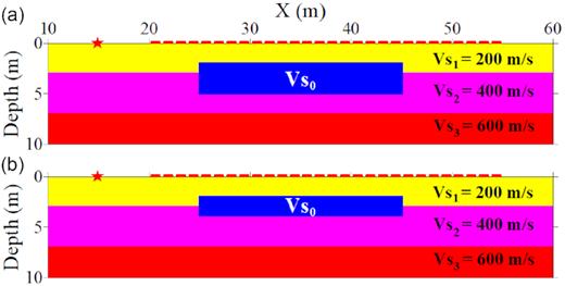
S-wave velocity model used to compare the three single objective functions. Asterisk and dashed line represent the location of the source and receivers, respectively. (a) is the true model and the initial model used in the consistent case, (b) is the initial model used in the inconsistent case.
We change Vs0 from 100 to 550 m s−1 in the model and calculate the three single objective functions corresponding to each model (solid lines in Fig. 2), respectively. It can be seen that ϕ1 has the narrowest region of global minima, which ranges from 240 to 400 m s−1. The sizes of the global minima region are much wider in ϕ2 and ϕ3, which range from 170 to 490 m s−1 and 225 to 550 m s−1, respectively. The shape of ϕ2 is more convex compared to the other objective functions. Three objective functions show relatively high consistency in the region where Vs0 is close to its true value and relatively low consistency when Vs0 is far away from its true value. It suggests that a small ϵ value is enough when an appropriate initial model is used, while bigger ϵ values should be adopted when poor initial models are provided.
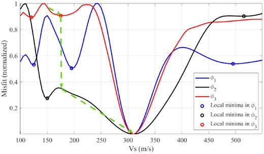
Three objective functions for Vs0 ranging from 100 to 550 m s−1 in the consistent case. Circles represent the locations of local minima. Dashed arrows schematically illustrate the solution path of MOWI when an initial model of Vs0 = 150 m s−1 is chosen.
Local minima exist in all three objective functions (circles in Fig. 2), showing that none of the three single-objective FWIs is intrinsically immune to the problem of local minima. There is no local minimum that locates identically at the same location in multiple objective functions. It indicates that MOWI is able to avoid or jump out of these local minima by using multiple objective functions simultaneously. For example, if we start an inversion at the point that Vs0 = 150 m s−1, all three single-objective functions will be trapped into local minima. If we start at the same point by using MOWI, the inversion will first ‘converge’ to the local minimum point in ϕ3 at Vs0 = 175 m s−1. Then, MOWI will start to optimize ϕ2 and successfully converge to the global minimum (dashed arrows in Fig. 2). Therefore, the convergence of MOWI to the global minimum is much less dependent on the initial model compared to the single-objective FWIs.
3.2 Shapes of objective functions in an inconsistent case
We use the same true model to generate the observed data but slightly change the structure in the model for synthetic data to create an inconsistent example. We decrease the thickness of the rectangular anomaly from 3 to 2 m in the model and put it at a depth between 2 and 4 m (Fig. 1b). So there is a systematic error between the true model and the synthetic models for simulation. A similar situation might happen when incorrect prior information is provided or an inaccurate model parametrization is performed.
Similarly, we simulate the waveforms of the model whose Vs0 ranges from 210 to 410 m s−1 and calculate their corresponding misfit values. Unlike what we have observed in the consistent case that all three objective functions have the same global minimum located at the true Vs0 value (Fig. 2), three objective functions no longer have a common global minimum point (Fig. 3). ϕ1 and ϕ3 share a same global minimum point located at 295 m s−1 while the global minimum in ϕ2 locates at 315 m s−1. All solutions between these two global minimum points are the Pareto solutions. Therefore, we will obtain many (infinite) Pareto solutions instead of one unique optimal solution. Assuming that all Pareto solutions are uniformly distributed on the Pareto front (area between two dotted lines in Fig. 3) and are fully sampled, it would provide the probabilistic distribution of the optimal solutions, which suggests that the optimal solutions locate around 305 m s−1 with an uncertainty of 33.3 m2 s−2 (i.e. 305 m s−1 ± 5.8 m s−1, where 5.8 is the corresponding standard deviation). Similar systematic errors in FWI might be seen in real-world cases due to the existence of noise and the simplifications made in the forward theory (e.g. ignoring viscosity and/or anisotropy). This example shows that MOWI is able to quantitatively estimate the uncertainty in the inverted model parameters.
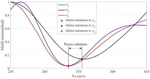
Three objective functions for Vs0 ranging from 210 to 410m s−1 in the inconsistent case. Circles represent the locations of global minima.
4 SYNTHETIC INVERSION TESTS
We use a 2-D heterogeneous model to test the validity and performance of MOWI. The true model consists of a homogeneous density of 2000 kg m−3. The P-wave velocity linearly increases from 320 m s−1 at the free surface to 680 m s−1 at the bedrock located 8 m deep. The S-wave velocity (Fig. 4a) generally increases with depth, and contains one spherical low-velocity body and two high-velocity bodies of irregular shapes at a depth from 2 to 5.5 m. Forty-eight two-component (vertical and inline horizontal components) receivers are placed along the free surface with an interval of 1 m and the first receiver located at X = 13 m. A total of nine vertical-force sources (source time function simulated by a 30 Hz Ricker wavelet) are generated with a source spacing of 6.4 m (asterisks in Fig. 4).
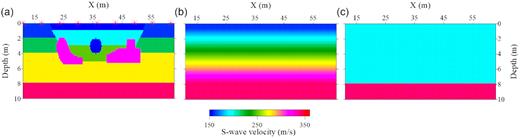
(a) True S-wave velocity model for the synthetic inversion tests. Asterisks represent the locations of the sources. (b) Linear-gradient initial model in the first inversion test. (c) A layer over a half-space initial model in the second inversion test.
We perform a mono-parameter inversion in the synthetic example where only the S-wave velocity is updated. This is because Rayleigh wave is much more sensitive with respect to S-wave velocity compared to the other parameters (Groos et al. 2017). The other parameters, including the source-time function, are kept as their true values during the inversion. Two different initial models, including a linear-gradient model and a layer over a half-space model (Figs 4b and c), are used to perform the two inversion tests, respectively. The l2 model misfit of the second initial model is approximately two times the value corresponding to the linear-gradient one.
4.1 Linear-gradient initial model
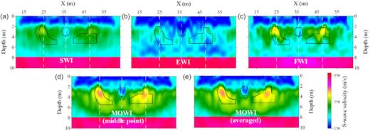
We apply SWI (ϕ3), EWI (ϕ2) and conventional least-squares FWI (ϕ1) to the synthetic example with the linear-gradient initial model, respectively. All the inverted models (Figs 5a–c) delineate the main structures of the model, including the low- and high-velocity bodies. It indicates that each waveform inversion can independently reconstruct the subsurface model to a good level. Comparatively speaking, the low-velocity body is better reconstructed, while the shapes of the high-velocity bodies are poorly resolved, especially for their lower boundaries. Besides, the layer interface at 1 m deep is contaminated by some vertical-stripped artefacts.
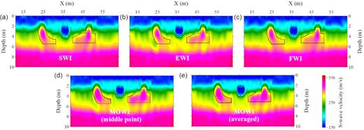
Inversion results of the first synthetic test. Panels (a), (b) and (c) are the results of SWI, EWI and least-squares FWI, respectively. Panels (d) and (e) are the inversion results of MOWI. The black lines delineate the locations of the low- and high-velocity bodies. The quality of the inversion results of MOWI is better than the results estimated by single-objective FWIs.
We also applied MOWI to the synthetic example by using an ϵ value of 1.1 and switching criterion II. MOWI shares the same solution path with SWI in the first 16 iterations and starts to optimize ϕ2 at the 17th iteration (Fig. 6). SWI, EWI and FWI converge to their final solutions after 26, 36 and 31 iterations, respectively, while MOWI stops to probe the model space until maximal iteration number (100 in this example) is reached. It can be seen that all the single-objective solutions are dominated by some of the MOWI solutions, and we obtain a total of 11 local Pareto solutions. Taking the visually middle point of the estimated Pareto front as an example (Fig. 6), it dominates all the three solutions obtained the single-objective FWIs, and has a 55 per cent decrease in ϕ3 compared to the solution of SWI, a 44 per cent decrease in ϕ2 compared to that of EWI and a 16 per cent decrease in ϕ1 compared to that of least-squares FWI (Fig. 6), respectively. It shows that single-objective FWIs have prematurely converged to local minima.
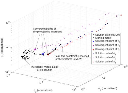
Solution paths of MOWI and different single-objective FWI approaches.
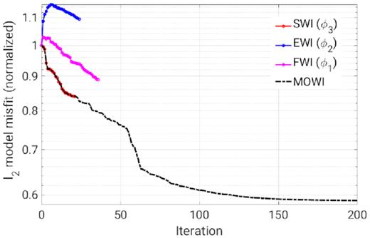
We also compare this visually middle-point solution and the averaged Pareto solution obtained by MOWI to the single-objective solutions (Fig. 5). The MOWI results better resolve the shape as well as the values of the two high-velocity bodies compared to single-objective FWIs, especially for the horizontal lower boundaries of the high-velocity bodies. The inversion results of MOWI also reconstruct the layer interface at 1 m deep and contain much fewer fluctuations (artefacts) compared to the results of single-objective FWIs. Fig. 7 shows the evolution of model misfit (l2) in MOWI and single-objective FWIs. The model misfit (error) generally decreases with increasing iteration in all the methods, and the final result of MOWI has around 10 per cent lower model error compared to the single-objective FWI results.
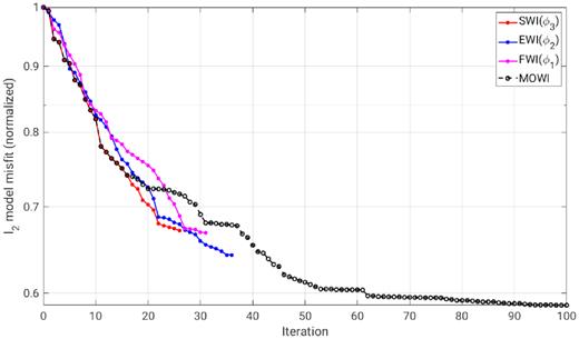
Evolution of l2 model misfit of MOWI and single-objective FWIs in the first inversion test.
In order to have a better estimation of Pareto front, we rerun MOWI by changing the ϵ value (1.0 or 1.1) and/or switching criterion (I or II) and obtain 11 ‘global’ Pareto solutions by evaluating the non-dominance of all solutions. Only 4 of the 11 local Pareto solutions estimated by the previous solution path (Fig. 6) stay as the ‘global’ Pareto solutions.
We calculate the uncertainty of the middle-point model as well as the variance of the models on the estimated Pareto front grouped by the eleven ‘global’ Pareto solutions (Fig. 8). Both two uncertainty maps show a similar structure but the middle-point model has relatively higher values (uncertainty) compared to the averaged model (Figs 8a and b). Both of them show that the optimal models have a relatively high consistency (variance ≤ 5 m2 s−2) in most of the subsurface area. The low-consistency areas (variance ≥ 10 m2 s−2) mainly exist in the left- and right-hand corners of the models (areas with arrows in Fig. 8), as well as inside and below the two high-velocity bodies. The low-consistency areas coincide with the low-illumination areas and have relatively high trade-off effects among multiple objective functions. The variance of the optimal models (Fig. 8) suggests that the inclusion of the low-velocity body in the inversion result is fairly credible, while the result inside and below the high-velocity bodies is less reliable in the reconstructed model. It is because that the low-velocity body locates relatively shallower compared to the high-velocity bodies so that more surface-wave energy has propagated through it. It also agrees with the results presented in Nolet & Dahlen (2000) that high-velocity structures are more difficult to resolve compared to low-velocity structures since wave front distortion caused by the high-velocity anomalies can be healed much faster than the distortion caused by the low-velocity anomalies.
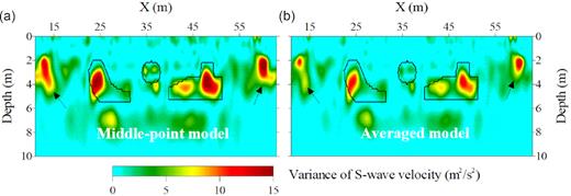
Variance of the models on the estimated ‘global’ Pareto front. (a) and (b) represent the variance of the middle-point model (Fig 5d) and averaged model, respectively.
We also calculate the model misfit of all ‘global’ Pareto solutions (black line in Fig. 9). The maximal difference among their model misfits is less than 2 per cent (11th Pareto solution and its value in Fig. 9), which again show a high consistency of the Pareto solutions in the model space. The data misfit values, however, differs more compared to that of the model misfit, especially in ϕ1 whose values differ more than two times among the Pareto solutions (magenta dashed line in Fig. 9). Overall, the model misfit is generally proportional to data misfits ϕ2 and ϕ3, while no clear relationship can be identified between model misfit and data misfits ϕ1 among the Pareto solutions.
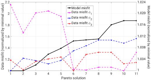
Model and data misfits of the ‘global’ Pareto solutions. Their values correspond to the right- and the left-hand axes, respectively. Model misfit generally increases from left to right.
Fig. 10 shows a comparison between the data and the model misfits for all models (solutions) along three MOWI solution paths (around a total of 300 solutions). Overall, we can see a clear linear relationship between the logarithm of data misfit and the model misfit in all three objective functions. This linear relationship, however, no longer holds for ϕ1 when model misfit is relatively low (i.e. model misfit < 0.65 in Fig. 10a). It shows that the reduction in ϕ1 less likely guarantees the reduction of model misfit compared to ϕ2 and ϕ3 when the model misfit is already low. Most of the Pareto solutions have very low model misfit, and the models with the lowest misfits are successfully included in the Pareto solutions. It again shows the validity of using MOWI for subsurface imaging.
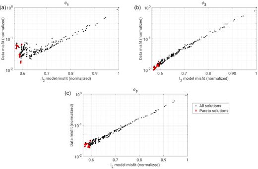
Model and data misfits of all solutions. Their values are normalized by the misfit values corresponding to the initial model.
4.2 A layer over a half-space (LOH) initial model
Similarly, we perform an inversion test by using the poor initial model (LOH model, Fig. 4c). We also increase the peak frequency of the Ricker wavelet to 35 Hz to make the inversion more challenging. Since the objective functions are more inconsistent when the initial model is far away from the true model, we choose an ϵ value of 1.2 and a maximal iteration number of 200 in MOWI.
The FWI, EWI and SWI converge after 36, 24 and 21 iterations, respectively, while MOWI stops when the maximal iteration number is reached. All single-objective FWI results reconstruct a low-velocity layer near the free surface (Figs 11a–c). Due to the poor initial model, none of the single-objective FWI results can nicely reconstruct the high- and low-velocity bodies. However, the inversion results of MOWI successfully delineate the existence and locations of the low- and high-velocity bodies (Figs 11d and e). Besides, they also reconstruct the flat layer interface at 1 m deep, which is not reconstructed by any of the single-objective FWIs.
Inversion results of the second synthetic test. (a), (b) and (c) are the results of SWI, EWI and FWI, respectively. (d) and (e) are the inversion results of MOWI. The black lines delineate the locations of the low- and high-velocity bodies. The white dashed lines represent the locations of three 1-D profiles through the high- and low-velocity bodies.
Fig. 12 shows the evolution of l2 model misfit obtained by the single-objective FWIs and MOWI. Although EWI successfully decreases its data misfit value (ϕ2), its final result has a greater model misfit compared to the initial model. SWI and FWI reduce the model misfit with 16 and 11 per cent in their final results, respectively. MOWI reduces 30 per cent of the model misfit after 60 iterations and finally decreases more than 40 per cent of the model misfit. It shows that MOWI outperforms single-objective FWI in reconstructing near-surface model by using shallow-seismic data. Besides, it also shows that MOWI is less dependent on the initial model compared to single-objective FWI.
Evolution of l2 model misfit of MOWI and single-objective FWIs in the second inversion test. The model misfit of the LOH initial model is approximately two times the value of the linear-gradient initial model in the first inversion test (Fig. 7).
Fig. 13 shows the comparison of three 1-D S-wave velocity profiles through the high- and low-velocity bodies. All inversion results reconstruct a low-velocity top layer, which is not included in the initial model. The EWI result fails to provide meaningful information about the high- and low-velocity bodies (blue lines in Fig. 13). The FWI and SWI results show the existence of the two high-velocity bodies but do not reconstruct the low-velocity body appropriately (green and magenta lines in Fig. 13). The MOWI result delineates the locations of the low- and high-velocity bodies to a good level (solid black and red lines in Fig. 13) and shows better agreement to the true model compared to the results estimated by the single-objective FWIs. All inversion results fail to reconstruct the structures deeper than 5 m because the surface wave energy mainly propagates within a depth shallower than half of its wavelength (approximately 5 m in this case).
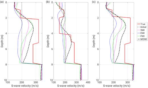
Comparison of three 1-D S-wave velocity profiles through the high and low-velocity bodies. Their locations correspond to the three dashed lines in Fig. 11.
Fig. 14 shows the data comparisons between the observed and synthetic data of the first shot gather in their waveforms (ϕ1), waveform envelopes (ϕ2) and f–k spectra (ϕ3). The waveform corresponding to the initial model is more than a wavelength away from the observed data in the far-offset traces (blue and black lines in Fig. 14a). It indicates a high possibility of being cycle skipped if we start a conventional FWI with this model. The synthetic data nicely fit the observed data in all three objective functions in the MOWI result, indicating that multi-objective optimization has been done by the modified ϵ-constraint method.
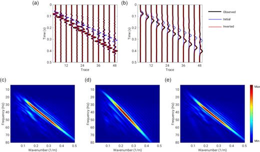
Comparison between the observed and synthetic data of the first shot gather (vertical component) in different objective functions. Panels (a) and (b) represent the comparison between the waveforms and waveform envelopes, respectively. Panels (c), (d) and (e) are the f–k spectra of the observed data, synthetic data of the initial model, and the synthetic data of multi-objective inversion result (middle-point solution of MOWI), respectively.
Fig. 15 compares the data residual corresponding to the initial model and the inversion results estimated by the single-objective FWIs and MOWI. The FWI, EWI and SWI results have the lowest data residual in their corresponding objective functions among the single-objective FWI results (i.e. Fig. 15d has the lowest waveform residual among Figs 15d, g and j, Fig. 15h has the lowest waveform envelope residual among Figs 15e, h and k, and Fig. 15l has the lowest residual in the f-k spectrum among Figs 15f, i and l). The FWI and SWI simultaneously decrease the data residual in all three objective functions, however, the EWI increases the data residual (misfit value) in ϕ3 (Figs 15c and i). It indicates that the objective functions ϕ1 and ϕ3 are more consistent while the objective function ϕ2 is less consistent with the other objective functions. The data residual of MOWI is consistently low in all three objective functions and is lower compared to the single-objective FWI results. It shows that MOWI outperforms single-objective FWI in reducing data misfit.
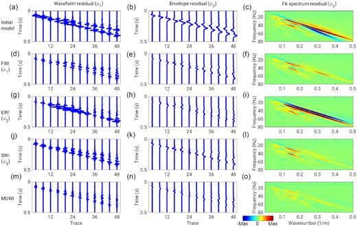
Comparison of the data residual in the vertical component of the first shot gather. Three columns represent the data residual of the waveform (ϕ1), waveform envelope (ϕ2) and f–k spectrum (ϕ3), respectively. Five rows represent the data residual corresponding to the initial model and the results estimated by FWI, EWI, SWI and MOWI (middle-point solution), respectively.
5 DISCUSSION
We propose to use a sequence from ϕ3 to ϕ2 to ϕ1 in the modified ϵ-constraint algorithm to optimize the multi-objective function. We also try another sequence from ϕ2 to ϕ3 to ϕ1 in the two synthetic inversion tests (Fig. 16). Their results fail to find a non-dominated solution compared to our proposed sequence; however, they still provide useful information about the subsurface model. The estimated results are more accurate compared to the models estimated by single-objective FWIs but less accurate compared to the models estimated by MOWI with our proposed sequence (Fig. 16 compared to Figs 5 and 11).
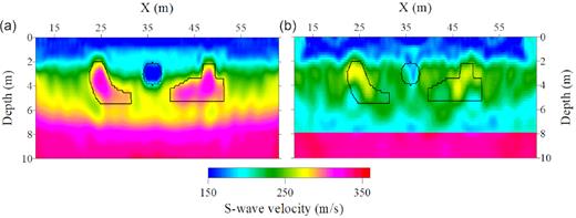
Averaged S-wave velocity model of the local Pareto solutions estimated by using a sequence from ϕ2 to ϕ3 to ϕ1 in the modified ϵ-constraint method. (a) and (b) are the results starting from the linear-gradient model and the LOH model, respectively.
As shown in the synthetic inversion tests, the sequence from ϕ3 to ϕ2 to ϕ1 in the modified ϵ-constraint algorithm provides lower data and model misfits compared to the other sequences. Since the least-squares misfit (ϕ1) has been proven more ill-posed compared to the other two misfits (e.g. Pérez Solano et al. 2014; Yuan et al. 2015; Pan et al. 2019), it suggests not to start the inversion sequence with ϕ1. As shown in the inconsistent numerical example and the second inversion test (Figs 3 and 15), the envelope objective function (ϕ2) is less consistent with the other two objective functions, which also makes it less meaningful to start the with ϕ2. Taking all considerations mentioned, we recommend using the sequence from ϕ3 to ϕ2 to ϕ1 in the modified ϵ-constraint algorithm to optimize the multi-objective function.
We adopt the modified ϵ-constraint algorithm mainly due to its simplicity. This algorithm, however, does not fully exploit the potential of MOWI since it only uses gradient information from one objective function at every iteration. The inversion may converge faster if multiple gradients could be used simultaneously. Thus, the design of a cost-effective optimization algorithm for MOWI deserves further investigation.
6 CONCLUSIONS
We have proposed a MOWI on shallow-seismic data to reconstruct near-surface models equipped with uncertainty analysis. We used three different criteria to quantify data similarity and tried to minimize them simultaneously via a modified ϵ-constraint algorithm. We compared the shapes of multiple objective functions in both consistent and inconsistent synthetic cases, respectively. The consistent case showed that MOWI is less dependent on the initial model compared to single-objective waveform inversions. The inconsistent case showed that MOWI could appropriately estimate the probabilistic distribution of optimal models. We also applied MOWI to synthetic inversion tests with different initial models and compared MOWI solutions to those obtained by single-objective waveform inversions. They showed that MOWI converges to better results and is less dependent on the initial model compared to the conventional methods. Besides, the variations of optimal solutions quantitatively showed the uncertainty of the inversion result. Other characteristics of MOWI, such as its combination with hierarchical strategy, require further studies.
ACKNOWLEDGEMENTS
The authors thank Thomas Hertweck and Martin Pontius for internal review and fruitful discussion. The authors also thank the editor F. Simons and three anonymous reviewers for their constructive comments. We gratefully acknowledge financial support by the Deutsche Forschungsgemeinschaft (DFG) with Project-ID 258734477 - SFB 1173.
REFERENCES
Author notes
Now at: University of Mannheim, 68131 Mannheim, Germany.
