Temporal changes of seismic velocities in the San Jacinto Fault zone associated with the 2016 M_w 5.2 Borrego Springs earthquake Free

SUMMARY

1 INTRODUCTION

Co- and post-seismic temporal changes of seismic velocities associated with earthquakes of different sizes and in different tectonic settings have been studied using earthquake waveforms (e.g. Poupinet et al.1984; Peng & Ben-Zion 2006; Sawazaki et al.2009; Nakata & Snieder 2012; Roux & Ben-Zion 2013) and ambient noise cross correlations (e.g. Brenguier et al.2008a, 2014; Froment et al.2013; Obermann et al.2014; Hobiger et al.2016). Recent advances in deployments of dense seismic arrays around fault zones together with developments in analysis techniques provide improved opportunities to track temporal changes of seismic velocities in fault zone regions. The San Jacinto fault zone (SJFZ) is one of the most seismically active fault zones in southern California (e.g. Hauksson et al.2012; Ross et al.2017a; Ben-Zion & Zaliapin 2019), and is capable of producing large M_w > 7.0 earthquakes (e.g. Peterson & Wesnousky 1994; Onderdonk et al.2013; Rockwell et al.2015). Several M_w > 5 earthquakes occurred during the past decade in the complex trifurcation area of the SJFZ (Fig. 1a) associated with its three major fault branches, including the 2016 M_w 5.2 Borrego Springs (BS) earthquake with a hypocentre at ∼12 km depth. Analysis of source properties of the 2016 BS event indicate that it had significant directivity to the northwest (Ross et al.2017b). This inference is supported by the strongly asymmetric distribution of aftershocks of the BS event to the northwest of the main shock epicentre (Fig. 1).

Figure 1.

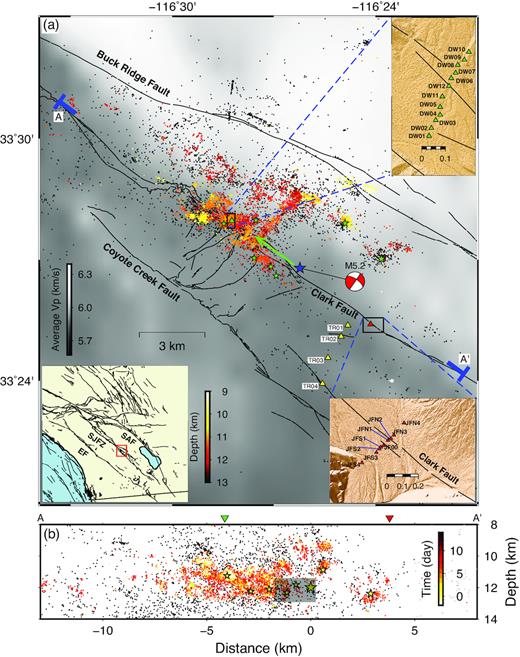
(a) Map of the trifurcation area of the San Jacinto Fault Zone (SJFZ) and fault zone linear arrays (DW in green, JF in red) analysed in this study. The average P-wave velocity over the depth range 1–7 km based on tomographic results of Allam & Ben-Zion (2012) is shown as the background colour (grey—slow and white—fast). The blue star, beach ball and green arrow indicate the epicentre location, focal mechanism and rupture directivity of the 2016 M_w 5.2 Borrego Springs earthquake. Aftershocks detected and relocated by Ross et al. (2017a) are coloured by depth, whereas the green stars indicate M_w 3.0 + aftershocks. The regional background seismicity during 2015–2016 is denoted as black dots. Surface traces of the San Jacinto fault in the trifurcation area are shown as black lines. The top and bottom right insets contain the zoom in of the station configuration for the DW and JF arrays, respectively. (b) Depth section of hypocentres projected along the cross-section AA’ with aftershocks coloured by the time relative to the main shock (largest yellow star). The shaded grey area represents a region in which more than 0.5 m of slip occurred during the main shock according to Ross et al. (2017b). The M_w > 3 aftershocks are shown as stars scaled with respect to the corresponding magnitude, and the black dots indicate locations of the background seismicity occurred during 2015–2016. The green and red triangles denote the locations of JF and DW arrays, respectively.

Open in new tabDownload slide

Five linear arrays consisting of 6–12 stations with an average station spacing of ∼20–40 m were deployed across different sections of the SJFZ (Vernon & Ben-Zion 2010). These include two arrays at Jackass Flat (JF) and Dry Wash (DW), which cross the main Clark branch of the SJFZ about 2–3 km to the northwest and southeast from the epicentre of the 2016 BS earthquake (Fig. 1). In this paper, we use ambient seismic noise recorded by these two linear arrays to analyse temporal changes of seismic velocities associated with the 2016 BS event. Regional tomographic images of the region (Allam & Ben-Zion 2012; Allam et al.2014; Zigone et al.2015; Fang et al.2016) show a contrast of seismic velocities across the Clark fault with the southwest side being slower in the top few kilometres (background grey scale in Fig. 1a). Theoretical studies of bimaterial ruptures and the observed velocity contrast imply a likely preferred propagation direction of earthquake ruptures in the area to the NW (e.g. Weertman 1980; Ben-Zion & Andrews 1998; Ampuero & Ben-Zion 2008) that is consistent with the observed directivity of the 2016 BS event. Fault zone imaging results at the JF and DW sites (Qiu et al. 2017a,b) suggest that both arrays cross the main seismogenic fault; however, the fault zone structures in the top few kilometres have different properties below the two arrays. Based on observation and modelling of fault zone trapped waves and delay time analysis of body waves, the JF array to the southeast of the BS event epicentre is situated in ∼200-m-wide fault damage zone with ∼35 per cent reduction of shear wave velocity relative to the host rock (Qiu et al.2017a). In contrast, delay time analysis and lack of clear trapped waves indicate a more localized, that is considerably narrower than 200 m, fault zone structure at the DW array situated to the northwest (Qiu et al.2017b). The configuration of two across-fault linear arrays at the opposite along-strike directions of the 2016 BS event epicentre provides a unique opportunity to investigate how the fault damage zone responds to a nearby moderate earthquake with rupture directivity.

Ambient noise correlation (ANC) techniques have been used extensively to image the subsurface between pairs of stations (e.g. Campillo & Paul 2003; Shapiro & Campillo 2004; Shapiro et al.2005; Zigone et al.2019). However, variations in properties of the noise sources (e.g. Kedar & Webb 2005; Stehly et al.2006) can bias the reconstructed waves. Using scattered arrivals in the coda part of the cross correlations (e.g. Snieder et al.2002; Grêt et al.2006; Sens-Schönfelder & Wegler 2006; Brenguier et al. 2008a,b; Hillers et al. 2015a,b) is less sensitive to biases associated with changing source properties (Colombi et al.2014). In this study, we use coda waves of the ANC to estimate seismic velocity changes at different coda lapse times. This is done in different frequency bands that provide proxies for the depth extent of the temporal changes (e.g. Obermann et al.2016; Yang et al.2019).

In the next section, we describe the data and pre-processing steps used to obtain daily cross correlations. A denoising technique (Moreau et al.2017) is applied to improve the data quality. We use both time-domain (stretching) and frequency-domain (doublet) methods to estimate changes of seismic velocities δv/v for different lapse times in the coda of the correlation tensor and different frequency bands. The pairwise δv/v time-series are averaged over all station pairs within each array. The resulting array-median δv/v are fitted with a combination of terms including a linear trend, co- and post-seismic effects, and periodic component (Section 4.1). Since seasonal δv/v in the SJFZ have been observed and discussed in Hillers et al. (2015a), we focus on the earthquake related (i.e. coseismic and post-seismic) δv/v effects, which are highlighted by removing the fitted linear and periodic terms. The dependence of co- and post-seismic signals on lapse time, component, frequency band and array location are examined in detail (Section 4.2).

For all frequencies, we find a strong inverse relation between the coseismic velocity reduction associated with the 2016 BS event and the coda wave window used to measure δv/v. The results suggest a much larger coseismic perturbation of seismic velocities within the fault damage zone beneath the two arrays compared to the surrounding rock. We also observe a substantial difference in the magnitude of coseismic velocity reduction and post-seismic recovery time between the low-frequency band 0.1–0.4 Hz and higher frequency bands. This frequency dependence may indicate velocity changes associated with different mechanisms at different depth sections, such as coseismic earthquake slip (deep) and excited waves (shallow). To further compare changes associated with the BS earthquake beneath the DW and JF arrays, we normalize the δv/v time-series by a proxy for rock susceptibility—the estimated amplitude of the seasonal variations. The resulting scaled coseismic velocity reductions show systematically larger values at the DW array for both low (0.1–0.4 Hz) and high (1–4 Hz) frequency bands, possibly related to the NW rupture directivity of the BS earthquake.

2 DATA AND PROCESSING

We use 2 yr (2015–2016) of three-component continuous waveforms with 200 Hz sampling rate recorded by two linear fault zone arrays located in the trifurcation area of the SJFZ. The JF array consists of 9 broadband stations, and the DW array has 12 short-period sensors. Both arrays with an aperture of ∼400 m are located almost symmetrically to each side of the epicentre of the 2016 BS earthquake (Fig. 1) and are capable of recording high quality ground motion from 0.1 to 10 Hz. The data from the JF array are analysed up to November of 2016 when the array was removed.

To retrieve high-quality Green's function estimates from continuous seismic records, transient signals generated by earthquakes and other large episodic sources have to be removed prior to correlation (e.g. Bensen et al.2007). To reduce computation time, we down sample the data to 40 Hz prior to the pre-processing. Here, we adopt the pre-processing procedure of Poli et al. (2012), Zigone et al. (2015) and Hillers et al. (2015a) to compute daily ANC. This includes large amplitude transients removal, spectral whitening and amplitude clipping. Trial and error analyses suggested an optimized preprocessing with a window length of 1-hr, 0.1–12 Hz frequency band for spectral whitening, and a threshold of 3.5 times the standard deviation in amplitude truncation. The 2016 BS event was followed by high rate of aftershocks that last for ∼2 weeks (Fig. S1). Wavefield changes associated with small aftershocks (e.g. M_w < 1.0) within the first 2 weeks after the main shock are difficult to fully suppress and can bias the high-frequency Green's function estimates (e.g. Obermann et al.2015). Daily correlation functions of all station pairs within each fault zone linear array are computed by cross correlating the pre-processed data.

To achieve ANC with sufficient signal-to-noise ratio (SNR) and quality (Fig. 2), remaining low quality daily correlations are first removed from the raw correlation matrix (Fig. S2). Previous studies show that filtering (e.g. Hadziioannou et al.2011; Stehly et al.2015) and substacking at each date over a time interval of ±d days (e.g. Brenguier et al.2008a) can increase the SNR of the correlation functions. In this paper, we use a Singular value decomposition (SVD) based Wiener filter (Moreau et al.2017) to denoise the daily ANC matrix, which significantly improves the SNR of each individual daily trace. A 2-D low-pass SVD based Wiener filter with a size of 10 d and five samples (0.125 s) along the date and correlation lag time dimensions was found to yield the best results. The 10-d window size results in a 2–3 d temporal smoothing (e.g. Hillers et al.2019). After these additional processing, we rotate the nine-component cross correlation tensor into a system of fault perpendicular (R), along fault strike (T) and vertical directions (Z).

Figure 2.

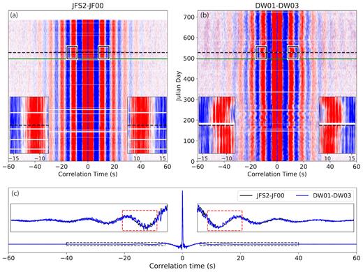
(a) Denoised daily ambient noise cross-correlations computed for year 2015 and 2016 between station pair JFS2 and JF00. The black dashed line indicates 10 June 2016, the origin time of the main shock, whereas the green line outlines the date one month before the main shock. Daily correlations below the green line are averaged to construct the reference trace shown in (c). The insets illustrate the zoom in of the reconstructed coda waves within the black boxes. (b) Same as (a) for station pair DW01–DW03. Obvious differences are observed in traveltimes of scattered arrivals before and after the main shock (black dashed lines). (c) Reference waveforms computed at station pairs JFS2–JF00 (black) and DW01–DW03 (blue). Coda waves between correlation times of 6 and 40 s (dashed black boxes) are zoomed in the insets. The red dashed boxes in the insets indicate the correlation time range used to plot the insets in (a) and (b).

Open in new tabDownload slide

We then stack the filtered daily correlations from the first day of 2015 to the day of the year that is 1 month before the 2016 BS earthquake (green line in Figs 2a and b) to generate the reference waveform (Fig. 2c). Ending one month before the 2016 BS event is to guarantee that velocity perturbations caused by the main shock and aftershocks are not included in the reference, and to not erroneously associate potential changes at the end of the stack period to medium changes.

To determine the part of the reference waveform that is dominated by coda wave signals above the noise level—coda wave window, we investigate the energy decay as a function of lag time. We assume that, different from the amplitude of direct waves that is governed by both geometrical spreading and attenuation, the coda waves are only affected by intrinsic and scattering attenuation, whereas the base noise level should be independent of the lag time. We stabilize the estimates by averaging the envelope functions over all available station pairs for the ZZ component and analyse the median envelope. A complete description of the coda wave lag time amplitude decay analysis can be found in the supplementary material (Appendix I and Fig. S3). Based on the fitting, the coda wave windows are 8 s ≤ |τ| ≤ 40 s for 0.1–0.4 Hz, 8 s ≤ |τ| ≤ 35 s for 0.5–2 Hz, 6 s ≤ |τ| ≤ 23 s for 0.75–3 Hz, and 5 s ≤ |τ| ≤ 22 s for 1–4 Hz. Here, we ignore the frequency band 0.25–1 Hz due to very low SNR levels (Fig. S4). Fig. S5 further validates that coherent coda arrivals can be extracted from ANC for frequency bands from 0.1–0.4 Hz up to 1–4 Hz within the determined coda wave window.

3 METHODOLOGY

3.1 Relative velocity change estimates

Instead of using individual scattered arrivals, a coda wave window is commonly used to stabilize the estimate. Since scattered arrivals with greater traveltime t have a correspondingly longer propagation path, the resulting estimations represent velocity perturbations averaged over larger areas surrounding the interstation path. Assuming a homogeneous relative velocity change, the obtained δv/v can be interpreted as the perturbation in medium properties for the sampled region.

We use the time-domain stretching method (Lobkis & Weaver 2003) and the frequency-domain doublet method (e.g. Poupinet et al.1984) to estimate δt/t from coda waves. Both methods compare a test trace to a reference trace and assume that temporal perturbations in coda wave traveltimes are small. The stretching method dilates or compresses coda waveforms in time domain, whereas the doublet method uses the moving window cross-spectral analysis (Clarke et al.2011) to estimate δv/v.

Both methods have their advantages and disadvantages. Spurious velocity change estimates may be observed using the stretching method when the coda wave amplitude spectrum varies with time (Zhan et al.2013). However, the time-domain technique processes the whole coda waveform at once and was found to yield more stable and precise estimation of δv/v with noisy data (e.g. Sens-Schönfelder & Larose 2008; Hadziioannou et al.2009). In contrast, the phase-based estimates of the doublet method are not affected by variations in the noise amplitude spectrum (Hadziioannou et al.2009; Colombi et al.2014). The frequency-domain method, on the other hand, suffers from problems such as cycle skipping (Mikesell et al.2015), in which phases are matched incorrectly between the coda waves in the test and reference traces, and the tradeoff between the Fourier transform window length and the accuracy of the δt/t measurement (Hadziioannou et al.2011). Since these two methods behave differently in the presence of fluctuations, consistency between estimations obtained from both techniques is indicative of the robustness of the resulting δv/v.

Noise recorded in the SJFZ environment is excited by different mechanisms: microseisms from ocean-continent interactions in the low-frequency band 0.1–0.4 Hz, and other natural and cultural sources (Hillers & Ben-Zion 2011; Inbal et al.2018) for higher frequencies (e.g. >1 Hz). Although the noise sources are not evenly distributed for frequencies above 0.1 Hz in the study region (e.g. Hillers et al.2013), the amplitudes of coda waves are similar at different time lags for all the frequency bands (Fig. S5). The coda waves are less symmetric in shape at frequencies above 0.5 Hz (e.g. Figs S5c–f). To minimize the effect of non-isotropic noise sources, we use the coda waves from both positive and negative time lags simultaneously to determine δv/v.

In contrast to previous studies using networks with apertures of tens of metres to hundreds of kilometres, the linear arrays analysed here are situated within fault damage zones that may yield larger temporal changes compared to the surrounding rock. For such localized temporal changes in rock properties, δt/t tends to be larger at early scattered arrivals and decreases with lapse time (e.g. Obermann et al.2016), because coda waves arriving at later lapse times averaged the seismic velocity variations over a larger area including host rock regions that are less affected compared to the near fault material. As a result, the underlying assumption of the doublet method that δt/t is independent of the lapse time t and can be estimated through linear regression using moving window is not fully compatible with the observation. The stretching method, on the other hand, provides estimates using the optimally dilated waveforms, which are dominated by large amplitude coda waves at early correlation time (Fig. S3).

3.2 Curve fitting

Figure 3.

Coherence and δv/v time-series obtained for (a) DW array using stretching method, (b) DW array using doublet method, (c) JF array using stretching method, and (d) JF array using doublet method. The grey curve represents the coherence (top panel) and δv/v (bottom panel) for each station pair. The blue solid and dashed curves denote the array-median and corresponding uncertainty calculated using results from all the station pairs. The stars denote the beginning and end of the coseismic period (Section 3.2). Measurements within the shaded area are magnified and shown in the inset. Coda waves from ZZ component within the coda wave window (i.e. 5–22 s; Fig. S3d) bandpass filtered at 1–4 Hz are used. The red and black dashed lines mark the origin time of the 2016 BS earthquake and the end of the stacking range used to construct the reference waveform, respectively.

Open in new tabDownload slide

The time resolution of the resulting δv/v curve is limited by the denoising filter (Moreau et al.2017), low quality daily ANC that are removed in the pre-processing steps (i.e. missing data points), and using the median of measurements obtained from all station pairs within an array. The stars in Fig. 3 outline a period, referred to below as the ‘coseismic period’. The shaded area is magnified in the insets and illustrates such smoothing effects. The maximum coseismic velocity reduction of the smoothed time-series (blue curves in bottom panels of Fig. 3) are not well aligned with the occurrence time of the 2016 BS event (red dashed lines). In addition, instead of a rapid drop, the coseismic velocity decreases rather gradually within the shaded time interval. The coseismic period is generally longer for DW array than that of JF array (Figs 3 and S6–S8), as recordings at the JF site are less affected by the aftershocks (coloured circles in Fig. 1).

Non-recovering velocity reductions after large earthquakes caused by material damage have been observed and modelled in previous studies (e.g. Peng & Ben-Zion 2006; Hobiger et al.2016). A complete post-seismic recovery is observed within ∼ 1 month after the 2016 BS event at 0.1–0.4 Hz (Fig. S6). However, at frequencies above 0.5 Hz, the obtained δv/v curves are not fully recovered due to insufficient long acquisition of seismic data after the BS event (Fig. 3, S7, S8) and thus cannot constrain possible persistent weakening effects. Therefore, the effect of a non-recovering coseismic velocity reduction is not included in our curve fitting analysis.

Figure 4.

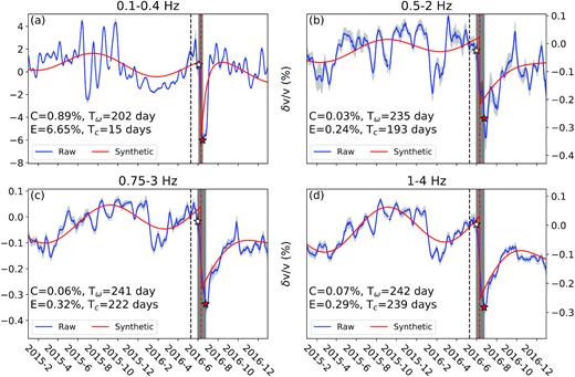
Array-median δv/v (blue) and corresponding best-fitting curve (red) of DW array at ZZ component using stretching method for frequency bands (a) 0.1–0.4 Hz, (b) 0.5–2 Hz, (c) 0.75–3 Hz and (d) 1–4 Hz. The grey area around the blue curve illustrates uncertainties of the obtained array-median δv/v. The shaded area between the stars denotes the coseismic period and measurements within are excluded from the curve fitting.

Open in new tabDownload slide

We estimate C, T_ω and T_c in eqs (2), (4b) and (5), and the corresponding uncertainties, for each array-median δv/v, using a nonlinear least square curve fitting algorithm from the SciPy package (e.g. Figs 4 and 5). Uncertainty of the array-median δv/v is computed as the standard deviation of the median (blue dashed curves in Fig. 3) and utilized to determine the weight of an estimate in curve fitting. The best-fitting linear trend (f_lin) and seasonal variations (f_per) are subtracted from the obtained δv/v to highlight the co- and post-seismic responses. Considering the fluctuations in δv/v obtained from different station pairs (e.g. grey curves in Fig. 3) and limited data for the post-seismic period, the purpose of the curve fitting is to provide first order estimates for the phase and amplitude of seasonal variations (Section 4.1.1), coseismic velocity reduction (Section 4.1.2) and post-seismic recovery time (Section 4.1.3). For a more precise analysis of coseismic and post-seismic components, δv/v curves after removing the modelled long-term variations (i.e. f_lin and f_per) are examined in Section 4.2.

Figure 5.

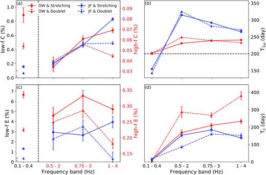
(a) Best-fitting parameter C, amplitude of the seasonal variation, as a function of frequency band. Results obtained using stretching and doublet methods are shown as dashed (triangles) and solid (circles) lines, whereas estimates for DW and JF array are displayed in red and blue, respectively. C values at the low-frequency band 0.1–0.4 Hz are shown in a larger scale (left-hand axis) compared to those at frequencies above 0.5 Hz (right-hand axis). Red ticks on the left y-axis illustrate the range of the right y-axis. (b) Best-fitting parameter T_1ω, initial phase of the seasonal variations, as a function of frequency. The black dashed lines indicate day of the year 200, at which the annual surface temperature in the SJFZ reaches the maximum. (c) Same as (a) for parameter E (coseismic velocity reduction). (d) Same as (b) for parameter T_c (effective post-seismic recovery time).

Open in new tabDownload slide

4 RESULTS

Fig. 3 shows the resulting δv/v obtained from ZZ correlations filtered at 1–4 Hz using coda waves in the time window of 5–22 s (see Figs S6–S8 for other frequency bands). Results of δv/v from the stretching (Figs 3a and c) and doublet (Figs 3b and d) methods show the same systematic temporal patterns. The results differ in the coherence values (lower for the doublet method) and in the amplitudes of the δv/v variations and the corresponding uncertainties. Systematic higher coherence values from the stretching method reflect the comparison of optimally dilated waveforms. Results from the doublet method used for comparison with the stretching method are shown in the supplementary materials.

Considering the small aperture (∼400 m) of the two fault zone arrays, the purpose of this section is to use the array-median δv/v time-series to infer a robust estimation of the seismic velocity perturbation in the fault damage zone, and analyse relations of the observed temporal patterns with the 2016 BS event and other natural loads that can be driven by temperature variations. While averaging δv/v time-series for the entire array suppresses the background variations, the array-median δv/v curve may yield less sharp coseismic velocity reduction. This is because the background fluctuation in δv/v varies in phase for different station pairs, so any rapid changes tend to be averaged over time. In addition, similar to the Fréchet kernel for finite frequency traveltimes (e.g. Dahlen et al.2000), the sampled volume and thus the sensitivity of coda waves to velocity perturbations in a heterogeneous medium increases both horizontally and vertically with lapse time (e.g. Obermann et al. 2013, 2016). The sensitivity halo for coda waves thus likely exceeds the size of the ∼200 m wide fault damage zone, particularly at low frequencies (e.g. 0.1–0.4 Hz) and longer lapse time (e.g. 30–40 s). A detailed study of δv/v measured for coda waves at different lapse times (Section 4.2.1) can provide constraint on rock susceptibility to perturbations in fault damage zones and the surrounding rock.

4.1 Results of curve fitting

Fig. 4 illustrates the curve fitting results of the array median δv/v time-series estimated for the DW array using the stretching method (see Fig. S10 for the doublet method; Figs S11, S12 for the JF array). ZZ component correlations and the frequency dependent coda wave windows shown in Fig. S3 are used here. The best-fitting parameters, amplitude (C) and phase term (T_ω) of seasonal components, post-seismic recovery time (T_c) and the measured coseismic velocity reduction (E) are indicated in the figure. The measurements for all the frequency bands, arrays, components and lapse time windows are well quantified by the modelled δv/v time-series. The fitness generally increases with frequency. In this section, we mainly focus on the best-fitting parameters shown in Fig. 5.

At 0.1–0.4 Hz, we find large amplitude periodic (30–40 d periodicity) fluctuations in δv/v between June and October of 2015 (e.g. Fig. 4a), particularly at the DW array. Peak-to-peak amplitude of the oscillation is comparable to the observed coseismic reduction in δv/v for both arrays. Based on the earthquake catalogue of Hauksson et al. (2012, updated to later years at the SCEDC 2013), there are no M_w > 3.0 earthquakes in the study region (Fig. 1a) between June and October of 2015. This large-amplitude transient fluctuation correlates well with the visible waveform perturbations in daily ANC computed for the station pair DW01–DW03 (Fig. 2b, between day of the year 100 and 300) and is responsible for the poor estimation of the seasonal variations (Fig. 4a). However, we do not observe fluctuations on that timescale in the higher frequency bands between 0.5 and 4 Hz. Since the amplitude of this signal decreases with lapse time (Section 4.2.1; Figs S13 a and b), we conclude that it is caused by spurious variations in the microseisms excitation pattern (Hillers et al.2015a).

4.1.1 Seasonal variations—parameters C and T_ω

The annual variation term f_per is characterized by the amplitude C and peak time T_ω. Best-fitting values of C (0.03–1 per cent) and T_ω (150–330 d) estimated from the DW and JF arrays using both methods are shown in Figs 5(a) and (b), respectively.

There are two broad possible causes for the derived seasonal variations in seismic velocities: changes in medium properties, such as crack density or fluid content, and variations caused by wavefield properties that are considered spurious (Zhan et al.2013). To identify the dominant driving mechanism for seasonal variations in the SJFZ, Hillers et al. (2015a) performed lapse time analysis and investigated the delay between the obtained seasonal variations and various relevant environmental records such as atmospheric temperature, wind speed and precipitation. They concluded that the δv/v variations in the SJFZ at 0.1–0.4 Hz are likely caused by wavefield changes. For the frequency ranges of 0.5–2 and 1–4 Hz, however, the results more likely reflect the medium response and the most plausible primary mechanism was inferred to be thermoelastic strain (e.g. Berger 1975; Ben-Zion & Leary 1986). We also perform lapse time analysis and show corresponding results in Figs S13 and S14. To clarify the primary mechanism, we examine the delay between the observed seasonal variations and annual air temperature. The surface temperature record is taken from the Piñon Flats observatory near the SJFZ (Hillers et al.2015a) and it reaches the maximum around day 200 of the year. Therefore, we use T_max = 200 (dashed black lines in Fig. 5b) as the peak time of the annual surface temperature for both array locations to roughly estimate the delay between the δv/v signals and the air temperature.

At the low-frequency band 0.1–0.4 Hz, we find large deviations between C values (eq. 5) based on different methods (circles versus triangles in Fig. 5a) or arrays (red versus blue in Fig. 5a). The differences in C values derived from the stretching and doublet methods indicate that the seasonal signals extracted from time- and frequency-domain are inconsistent. The systematic larger C value at DW array may reflect differences in array configurations and in situ conditions between the two arrays. In addition, the C values at 0.1–0.4 Hz yield significantly larger seasonal variations compared to the analysed higher frequency bands (Fig. 5a). On the other hand, very similar T_ω values (eq. 5) are obtained at the low-frequency band for both methods (Fig. 5b): the seasonal variations peak at T_ω ≈ 200 and 150 for the DW and JF arrays, respectively. The fact that the obtained T_ω values are equal or smaller than T_max (i.e. 200) rules out thermoelastic strain as the dominant mechanism for the observed seasonal variations. These observations are consistent with the conclusion of Hillers et al. (2015a) that seasonal variations at 0.1–0.4 Hz in the SJFZ region likely reflect changes in microseism excitation pattern rather than rock responses.

At higher frequency bands between 0.5 and 4 Hz, the values of C obtained from the stretching and doublet methods at both arrays are ∼0.05 per cent and generally increase with frequency (Fig. 5a). This magnitude of C values agrees with the seasonal variations in the SJFZ environment at 0.5–2 Hz reported in Hillers et al. (2015a, C ≈ 0.1 per cent). As shown in Fig. 5(b), consistent T_ω values are achieved using both the stretching and doublet methods. At the DW array, T_ω ≈ 240 for all three frequency bands and both methods, whereas the T_ω values for JF array are larger and decreases with frequency. With T_max = 200, there is a ∼40-d delay between the obtained seasonal δv/v at the DW array and the annual surface temperature. This average 40-d delay is expected for a thermoelastic effect in homogenous elastic half-space (Berger 1975; Tsai 2011; Richter et al.2014). At the JF array, the delay is longer (∼120 d at 0.5–2 Hz to ∼60 d at 1–4 Hz; Fig. 5b) compared to that at the DW array and the difference decreases with increasing frequency, which may reflect a thicker soil layer (Ben-Zion & Leary 1986).

We conclude that thermoelastic strain is the plausible primary mechanism for the observed seasonal variations in δv/v at frequency bands between 0.5 and 4 Hz. The decreasing phase change, between δv/v and temperature records, with increasing frequency at JF array is consistent with the fact that coda waves at lower frequencies are generally more sensitive to changes in deeper structures, associated with somewhat thicker effective unconsolidated layer for thermoelastic strain signal (e.g. Prawirodirdjo et al.2006; Ben-Zion & Allam 2013). The lack of such a trend in delay time at DW array may reflect different local fault zone structures beneath the arrays (Qiu et al. 2017a,b). No strong lapse time dependence is found in seasonal variations (Figs S13 and S14), suggesting the seasonal loadings, such as those driven by air temperature changes, are likely affecting an area that extends beyond the narrow fault damage zone.

4.1.2 Coseismic velocity reduction—parameter E

The coseismic velocity reduction, characterized by a rapid drop, stands out from the background long period variations in the obtained δv/v time-series (e.g. Figs 3 and 4). The parameter E (eq. 4a) indicates a first order estimate of coseismic velocity reduction before and after T₀, the time of the 2016 BS event. In general, the coseismic component is well estimated in all cases (Fig. 4 and S10–S12), but the results at the DW array yield less reliable coseismic estimates due to a large amplitude 2-week-long oscillation right after the event origin time T₀. It is interesting to note that we observe similar oscillations at the same time of the year in the year before (Fig. 4). This implies spurious effects of possible atmospheric pattern that affects ocean states and thus induces variations in noise wavefield. The 2-week-long oscillation in the δv/v curve at frequencies >0.5 Hz (shaded area in Figs 4b–d, S10b–d) may also reflect the influences of the aftershock sequences (Fig. S1). The aftershocks produce additional rock damage and excite waves that potentially cause both medium changes and wavefield variations that may only incompletely be removed by the applied pre-processing steps. Since most of the aftershocks occur beneath the DW array, the asymmetrical aftershock distribution is consistent with the observation that the coseismic δv/v reduction in the JF array results (Figs S11 and S12) can be estimated with a better fit.

Considering the potential biases in estimates of the absolute coseismic velocity reduction E, due to variations in the noise wavefield properties associated with the aftershock activity, we compare E values derived from different methods. At the low frequency band 0.1–0.4 Hz, the E estimated from the stretching method-based δv/v time-series is ∼2 times as large as that of the doublet method-based results for both arrays. The values of E are > 3 per cent at DW array and between 0.3 and 1.3 per cent at the JF array (Fig. 5c). Our results are much larger (>10 times) than that resolved at Parkfield between 0.1 and 0.9 Hz (∼0.1 per cent; Brenguier et al.2008a). At frequency bands between 0.5 and 4 Hz, the E value is ∼0.15–0.35 per cent for both arrays and methods (Fig. 5c). Our ∼0.2 per cent coseismic velocity reduction is comparable to those observed in fault zone environments in Japan and in the Salton Sea geothermal field between 0.5 and 4 Hz (Hobiger et al.2016; Taira et al.2018). These comparisons indicate that the coseismic changes in velocities occur mainly near faults at low frequencies (0.1–0.4 Hz) but are not limited to fault zone materials at higher frequencies (>0.5 Hz).

4.1.3 Post-seismic velocity recovery—parameter T_c

In Section 3.2, we modelled the post-seismic velocity recovery using an exponential function (eq. 4a), as the logarithmic function (eq. 3) suffers from an overshooting issue (Fig. S6) in curve fitting. The characteristic time T_c (eq. 4a) quantifies the post-seismic response with a larger value indicating a slower recovery. As discussed in Section 2, we have less than 6 month of data to constrain the post-seismic δv/v. When the time for a complete post-seismic recovery is longer than 6 months (i.e. ∼180 d), T_c could not be well constrained through curve fitting and often yields a large discrepancy between results from the stretching and doublet methods (Fig. 5d). In addition, the accuracy of the estimated post-seismic recovery time T_c also depends significantly on the quality of the estimation for the coseismic velocity reduction E, which is not well constrained for the DW array results due to a 2-week-long background oscillation immediately after the BS event. In general, both stretching and doublet methods show compatible trends in Fig. 5(d). At the low frequency band 0.1–0.4 Hz, T_c is ∼10 d for both arrays and methods. However, T_c estimates at the higher frequency bands are much larger. At the JF array, both methods suggest T_c ≈ 150 d from 0.5–2 Hz to 1–4 Hz. At the DW array, T_c values (∼200–300 d) are larger than those of JF array for both methods.

We then fit the corrected δv/v measurements—|${\skew{6}\tilde{f}_{{\rm{eq}}}}$| in a specific post-seismic time window (T_p1 < T < T_p2) with eq. (3), which is equivalent to the linear regression of |${\skew{6}\tilde{f}_{{\rm{eq}}}}(T - {T_0})$| on |$\ln ( {1 + T - {T_0}} )$|⁠. Note that the estimates of E₁ and E₂ can be sensitive to the selection of the post-seismic window, particularly for cases with insufficient long records (Fig. S15; frequencies >0.5 Hz). Therefore, we only discuss the results of this logarithmic post-seismic analysis for the frequency band 0.1–0.4 Hz, where a complete recovery is achieved in the obtained δv/v curve and is poorly fitted using an exponential function (e.g. Fig. 4a).

Fig. 6 shows the best-fitting logarithmic post-seismic recovery and corresponding estimates of coseismic velocity reduction E_log ( = E₁) and post-seismic recovery time T_log. A complete description of the determination of the time window used in the analysis can be found in the supplementary material (Appendix II). In general, |${\skew{6}\tilde{f}_{{\rm{eq}}}}( {T - {T_0}} )$| in the selected post-seismic window (grey dots within the black dashed lines in Fig. 6) yields a good agreement with the assumed logarithmic recovery (straight red dashed lines in Fig. 6). Since a complete recovery (blue dashed lines in Fig. 6) is achieved, T_log is well constrained (∼30 d) for both arrays and methods at 0.1–0.4 Hz.

Figure 6.

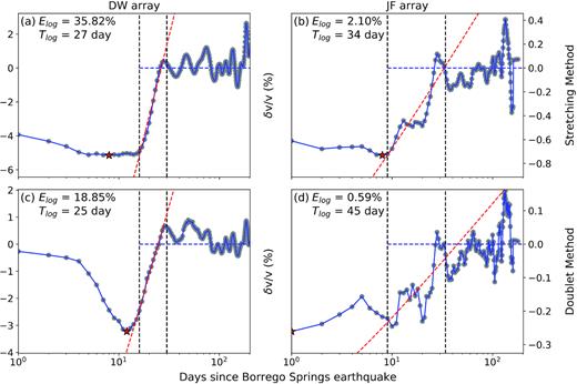
(a) EQ responses of δv/v curve (eq. 6) after the origin time of the 2016 BS earthquake (T > T₀) at 0.1–0.4 Hz for DW array shown as a function of |${\rm{ln}}( {1 + T - {T_0}} )$|⁠. The dashed lines outline the portion of data that show a clear logarithmic recovery (red dashed lines) and is used to estimate the coseismic velocity reduction E_log ( = E₁) and post-seismic velocity recovery time T_log (⁠|$= {e^{{E_1}/{E_2}}} - 1$|⁠; eq. 3). The horizontal blue dashed lines denote δv/v = 0. (b) Same as (a) for doublet method-based results. (c) Same as (a) for JF array. (d) Same as (b) for JF array.

Open in new tabDownload slide

The estimated coseismic velocity reduction E_log, however, is much larger than E estimated in Section 3.2, particularly at the DW array (e.g. E ≈ 6 per cent in Fig. 4a and E_log ≈ 36 per cent in Fig. 6a). This is because the coseismic velocity drop obtained from the δv/v curves is largest at 5–14 d after the BS event due to limitations in the time resolution (Section 3.2) and thus includes a partial recovery, whereas the refined fitting with the logarithmic function includes information on earlier parts of the recovery process and thus yields much larger total coseismic velocity changes. The estimates of E_log are based on the assumption of a constant rate of logarithmic recovery (i.e. E₂/E₁; e.g. slope of dashed red lines in Fig. 6). E_log can be even larger if the actual recovery is much faster at the early 2 weeks of the post-seismic period (T ≤ 14 d) than that indicated by measurements in the period of T > 15 d (dashed lines in Fig. 6).

4.2 Comparative analyses

In Section 4.1, the curve fitting results provide first order estimates of different components of the observed δv/v time-series. Best-fitting parameters achieved from different methods and frequency bands are compared, indicating robust co- and post-seismic responses associated with medium changes caused by the 2016 BS earthquake. In this section, we remove the modelled linear trend and seasonal variations (eq. 6) to highlight the earthquake related variations (i.e. EQ responses) in the observed δv/v.

4.2.1 Lapse time analysis

To analyse potential localized distribution of temporal changes of rock properties, δv/v is estimated as a function of lapse time τ using small moving windows of coda waves. Fig. 7 compares the EQ responses of δv/v and corresponding coherence estimates obtained using the stretching method. Several 10s-long moving time windows within the coda wave window are used. We use frequency bands 0.1–0.4 Hz and 1–4 Hz for the lapse time analysis as these results are clearest. In general, we observe very high consistency in co- and post-seismic responses from results for all lapse time windows. However, the coseismic velocity reduction decreases monotonically with lapse time of the moving window. Similar patterns are observed in results obtained using the doublet method (not shown here).

Figure 7.

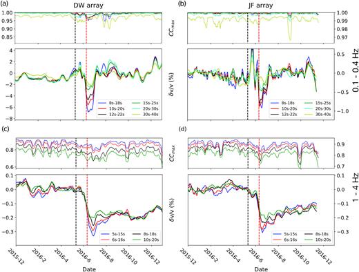
(a) Array-median coherence (top panels) and δv/v curves (bottom panels) measured using different lapse time windows (coloured curves) at 0.1–0.4 Hz. Model predicted linear trend and quasi-periodic components are removed from the δv/v curves (eq. 6). (b) Same as (a) for JF array at 0.1–0.4 Hz. (c) Same as (a) for DW array at 1–4 Hz. (d) Same as (a) for JF array at 1–4 Hz.

Open in new tabDownload slide

To further investigate the rate of decrease in the coseismic reduction with lapse time, we analyse the coseismic medium changes as a function of lapse time in Figs 8(a) and (b). Here we approximate the coseismic velocity reduction as the differences between the maximum and minimum δv/v values (e.g. stars in Fig. 3) within the coseismic period (shaded area in Fig. 3). For the low-frequency band 0.1–0.4 Hz, the rate at which the coseismic δv/v decreases with lapse time is much higher at DW than JF array, particularly at early lapse times. The rate is approximately the same for both arrays at 1–4 Hz. Coherence values, on the other hand, generally decrease with lapse time (Figs 8c and d) in both frequency bands, because of smaller SNR for coda waves at later lapse time (Fig. S3).

Figure 8.

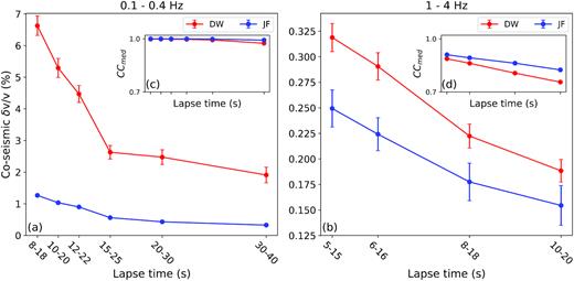
Lapse-time dependent coseismic velocity reduction and median coherence values derived from curves shown in Fig. 7. (a) Coseismic velocity reduction measured at 0.1–0.4 Hz as a function of lapse time window. Results for DW and JF array are shown in red and blue, respectively. (b) Same as (a) for 1–4 Hz. (c) Same as (a) for coherence values. (d) Same as (c) for 1–4 Hz.

Open in new tabDownload slide

We also compare the post-seismic recovery rate obtained for different lapse times. The coseismic velocity reduction is fully recovered with ∼30 d after the 2016 BS event for all lapse times at 0.1–0.4 Hz (Figs 7a and b). This rapid recovery likely reflects the faster post-seismic healing process in fault damage zones due to larger normal stress at greater depth. In general, we expect the fault damage zone to have a different healing rate compared to the surrounding host rock. However, the post-seismic δv/v yield the same recovery time for all lapse times (Figs 7a and b), despite the fact that coseismic velocity reduction (E) decreases with lapse time (Fig. 8a), which may indicate the coseismic velocity changes in the surrounding host rock are negligible compared to those within the fault damage zone at 0.1–0.4 Hz. At 1–4 Hz, the coseismic reduction is not fully recovered due to the limited period of recording (Figs 7c, d). The longer recovery time at higher frequency is also consistent with the smaller normal stress at shallower depth that delays the post-seismic healing process. In addition, we find the post-seismic δv/v recovers faster at earlier lapse time for the first 3–4 months after the 2016 BS event in Fig. 7(c). As δv/v at later lapse time are more sensitive to larger area, this observation at DW array may reflect a faster healing process close to fault damage zone during the first few months of the post-seismic period.

4.2.2 Frequency band

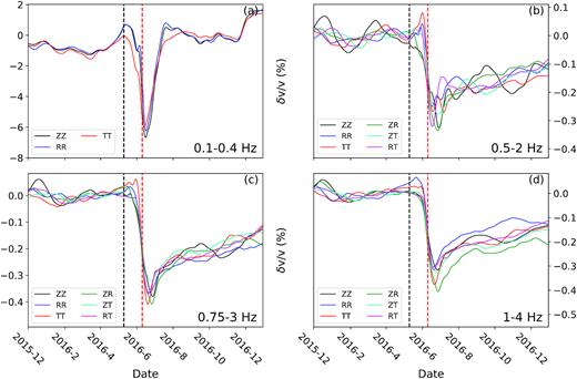
Fig. 9 shows the comparison of the EQ responses estimated at different frequency bands for both DW and JF arrays. The coseismic velocity reduction and post-seismic recovery at 0.1–0.4 Hz are significantly larger and faster than those at frequencies above 0.5 Hz, respectively. To estimate the depth range of the observed frequency dependent coseismic δv/v reduction, we need to consider the sensitivity of coda waves to local medium changes at depth. The coda is a mixture of body and surface waves in most crustal-like materials, and the partitioning between their contributions to the coda sensitivity depends on the heterogeneity of the medium and the coda lapse time (e.g. Obermann et al. 2013, 2016). For a first-order estimation, we ignore the contribution of body-wave sensitivity and assume the observed δv/v are most sensitive to medium changes at a depth of h_max that is proportional to the dominating wavelength λ.

Figure 9.

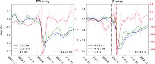
Comparison of the EQ responses of δv/v measured at four different frequency bands (colours) for the DW (left-hand panel) and JF (right-hand panel) arrays. ZZ component and stretching method are used. Median filter is applied to suppress the background fluctuations (transparent curves). The smoothed δv/v time-series are shown as solid curves. The right y-axis in red denotes the scale of the red curves (0.1–0.4 Hz).

Open in new tabDownload slide

We set h_max = λ/3 based on the depth sensitivity of surface wave phase velocity to shear wave velocity (e.g. Zigone et al.2015; Berg et al.2018). This relation suggests coda waves at lower frequency are more sensitive to changes in deeper structures. In this section, we provide a rough estimation on the depth of coseismic medium changes based on the surface wave depth sensitivity kernel and validate the assumption that the coseismic δv/v observed at lower frequencies are representative to seismic velocity perturbations in deeper structures.

At 0.1–0.4 Hz, the dominating frequency, f, is ∼0.14 Hz (secondary microseism), and the corresponding phase speeds, c, in fault damage zones at the DW and JF sites (e.g. Roux & Ben-Zion 2017; Berg et al.2018) are ∼3.2 km s^–1 for Rayleigh wave (e.g. ZZ component) and ∼3.4 km s^–1 for Love wave (e.g. TT component). Therefore, the apparent δv/v is most sensitive to medium changes at the depth of h_max = λ/3 = c/3f, which is ∼7–8 km. Similarly, for frequency bands above 0.5 Hz (i.e. f > 0.5 Hz), h_max is smaller than 2 km as c < 3 km s^–1 (Qiu et al.2019). Yang et al. (2019) found significant effects of shallow seismic velocity changes on phase velocities also of long periods (e.g. > 15 s) surface waves. Therefore, one cannot simply project the observed δv/v at a low frequency band (e.g. 0.1–0.4 Hz) to deeper structure without considering the measurements at higher frequency bands (e.g. 1–4 Hz). However, we observe that the largest coseismic velocity reduction (>0.5 per cent) followed by a significantly faster post-seismic recovery at the low-frequency band 0.1–0.4 Hz (Figs 5c and d). This implies that the observed coseismic velocity reduction at the low-frequency band is not significantly biased by medium changes in the shallow structure.

4.2.3 Different components

The recording component is indicative of the type of surface wave (e.g. ZZ—Rayleigh wave and TT—Love wave) reconstructed from ANC. The coda, however, is a mixture of scattered body and surface waves and thus does not have a simple relation between waveforms recorded at different components.

Fig. 10 illustrates the EQ responses estimated at different components using the stretching method for DW array (Fig. S16 for doublet method; Figs S17, S18 for JF array). Except for the low frequency RT and ZT results, we observe generally similar rapid coseismic velocity reductions followed by a post-seismic recovery associated with the 2016 BS earthquake for all components in each frequency band. Although the results include some variations in co- and post-seismic responses estimated at different components, there is no clear component-related pattern that can be easily interpreted. In general, the results obtained from different components indicate higher similarity at frequencies above 0.5 Hz than that at the 0.1–0.4 Hz. This is understood to result from coda waves at high frequencies contain high degree of mixing modes, that is multiple scattering, whereas the mixing is not as complete at the low-frequency band (Hillers et al.2013), due to the proximity of the study area to excitation region and the requirement of longer mean free path.

Figure 10.

Comparison of the smoothed EQ responses of δv/v measured using different components (colours) for DW array and stretching method at frequency bands (a) 0.1–0.4 Hz, (b) 0.5–2 Hz, (c) 0.75–3 Hz and (d) 1–4 Hz.

Open in new tabDownload slide

4.2.4 Array location

The observed δv/v time-series is determined by the loading mechanism and magnitude, and properties of the local structures like rock susceptibility beneath the stations. To compare the magnitude of coseismic loadings at the DW and JF sites, we remove effects of local structures in the observed coseismic δv/v. Since both arrays are located in fault damage zones with similar array geometry (insets in Fig. 1) and the inter-array distance is only ∼6 km, we assume that the amplitude of seasonal variations (C), either governed by medium or wavefield changes, is the same if the local conditions are similar at both sites. In other words, the observed C value is a first order proxy for the susceptibility of the fault damage zone, that is larger C value indicates material that is more susceptible to changes. Although the peak time T_ω of seasonal variations is different between two arrays, the discrepancy is associated with the phase and thus has less effect on the rock susceptibility. Therefore, we normalize the δv/v time-series by the corresponding best-fitting C value to account for local response.

Fig. 11 compares the normalized EQ responses for the DW (blue in Fig. 11) and JF (red in Fig. 11) arrays at 1–4 Hz. The top and bottom panels represent results using the stretching and doublet methods, respectively. Systematically larger coseismic reductions are observed at DW compared to those at JF for both methods and all three analysed components. The same pattern is also observed at the low frequency band 0.1–0.4 Hz (Fig. S19), but less clear at 0.5–2 Hz (Fig. S20) and 0.75–3 Hz (Fig. S21). Since the effects of site-specific structures are reduced, this observation suggests that the difference is associated with the NW rupture directivity of the 2016 BS earthquake (Fig. 1a) and the resulting larger amplitudes of seismic waves propagating towards the DW array.

Figure 11.

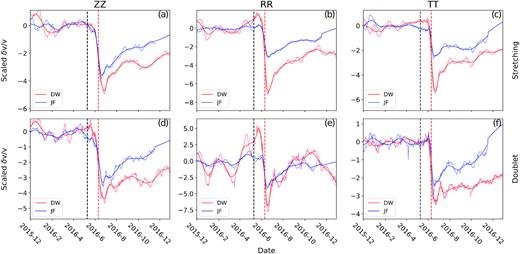
Comparison of the normalized EQ responses of δv/v measured at 1–4 Hz for the DW (red) and JF (blue) arrays. (a) The thin and thick curves represent the normalized raw and smoothed array-median δv/v, respectively. Results obtained from stretching method and ZZ component are used. Each δv/v curve is normalized by its corresponding best-fitting C value (seasonal variation amplitude; Fig. 3a). (b) Same as (a) for RR (fault perpendicular) component. (c) Same as (a) for TT (fault parallel) component. (d), (e), (f) same as (a), (b), (c) for doublet method.

Open in new tabDownload slide

5 DISCUSSION AND CONCLUSIONS

We monitor seismic velocity changes in the San Jacinto fault zone for a 2-year period (2015–2016) using ambient seismic noise recorded by two linear arrays with an aperture of ∼ 400 m. The two arrays at sites DW and JF are located within fault damage zones (Qiu et al. 2017a,b) at ∼3 km distance to the NW and SE of the 2016 M_w 5.2 Borrego Springs earthquake. Relative velocity changes (δv/v) are estimated using a time- and a frequency-domain method. Results from both methods are compared to distinguish medium changes from spurious variations. Clear seasonal variations and co- and post-seismic changes associated with the BS event are observed in the obtained δv/v time-series. A decreasing signal is often seen in the δv/v curve several days before the BS event (e.g. Figs 7a and d); this is not interpreted as a precursor signal as the trend is likely associated with the choice of the reference period (black dashed lines in Fig. 7), low coherence values, and background fluctuations. In Section 4.1, we obtained first order estimates of the amplitude and phase of seasonal variations, coseismic velocity reduction and post-seismic recovery time in various frequency bands. The estimated seasonal variations are later removed, and the highlighted co- and post-seismic δv/v curves at different coda wave windows, frequency bands, components and arrays were analysed in Section 4.2.

For seasonal variations (Section 4.1.1), the observed δv/v in the low-frequency band 0.1–0.4 Hz are likely spurious and governed by wavefield changes associated with annual variations in microseisms excitation. At higher frequencies between 0.5 and 4 Hz, the observed annual variations in δv/v beneath the DW and JF arrays are comparable to those reported in Hillers et al. (2015a). The delay between the obtained seasonal variations at these higher frequencies and the surface annual temperature record is ∼40–100 d, suggesting thermoelastic strain is a possible primary mechanism. However, the phase delay, between the observed seasonal variations in δv/v time-series and the assumed driving temperature changes, of the JF array are different from those of DW array, indicating effects of different local properties such as topography and fault zone structure.

The apparent coseismic velocity reduction is estimated to be ∼6 and ∼ 1 per cent at the DW and JF arrays, respectively, for the low frequency band 0.1–0.4 Hz and significantly smaller ∼0.2 per cent for frequencies between 0.5 and 4 Hz (Fig. 5c). Assuming the depth sensitivity of coda waves to medium changes is the same as that of surface waves to shear wave velocity, observations at 0.1–0.4 Hz represent medium changes at a depth of h_max = ∼7–8 km, whereas results at 1–4 Hz indicate perturbations in shallow materials, in the top 1–2 km. The ∼12 km depth of the 2016 BS hypocentre is comparable to the h_max estimate of ∼7–8 km at 0.1–0.4 Hz. Hence the relatively large coseismic velocity reduction at the low frequency band (>1 per cent) implies that the corresponding driving mechanism is the rock damage associated with coseismic earthquake rupture. For frequencies above 0.5 Hz, the observed medium changes are much shallower and thus likely associated with the straining of the radiated waves.

The coseismic velocity changes are expected to be higher within the fault damage zone, that is underneath the array, than in the surrounding rock (Peng & Ben-Zion 2006). This is supported by the obtained negative correlation between coda lapse time and coseismic δv/v reduction (Fig. 7; Section 4.2.1). As the coda wave sensitivity to velocity perturbations extends over larger regions at longer lapse time, the rate, η, at which coseismic δv/v decreases with coda lapse time t, is likely indicative of the fault zone width, that is a faster decrease of coseismic δv/v indicates a narrower fault damage zone. At 0.1–0.4 Hz, the rate η is much higher at DW (Fig. 8a), whereas it is similar for both arrays at frequencies above 0.5 Hz (Fig. 8b), suggesting a narrower fault damage zone beneath site DW than JF at greater depth, and similar fault zone width at shallower depth. This is consistent with observations that fault zones in general and the SJFZ in particular have decreasing width with depth (e.g. Ben-Zion & Sammis 2003; Zigone et al.2015), and differences in the imaged structures below the DW and JF arrays (Qiu et al. 2017a,b).

The localized coseismic velocity changes can also explain the observed large differences in the obtained coseismic velocity reduction E (eq. 4) between the stretching and doublet methods at 0.1–0.4 Hz (Section 4.1.2). Since the stretching method is performed in the time domain, the resulting coseismic δv/v is mainly governed by the velocity perturbation associated with the largest scattered arrival in the selected time window (Section 3.1), which is typically the arrival at the earlier lapse times (Fig. S3). The doublet method, on the other hand, is equivalent to a moving window cross-spectral analysis, in which δv/v is estimated through a linear regression of δt and t. As δt measured at different lapse time t is equally weighted, lower δv/v values are expected for the doublet method, due to biases of smaller δt/t at larger t. In addition, we find the largest discrepancy in coseismic δv/v between the two methods at 0.1–0.4 Hz from the DW array data (Fig. 5c). This is consistent with the observation that the highest rate η is also seen at the 0.1–0.4 Hz band at the DW array (Fig. 8).

To separate effects of the loadings from the local rock susceptibility, we normalize the observed δv/v time-series by the amplitude of seasonal variations (Section 4.2.4). Systematically larger coseismic velocity reductions are observed at the DW site compared to the JF site (Figs 11 and S19), which can be explained by the asymmetrical distribution of coseismic slip and wave excitation associated with the NW rupture directivity of the 2016 BS earthquake (Ross et al.2017b). This suggests that the observed coseismic velocity reduction obtained from noise-based seismic monitoring resolve directivity effects of the earthquake rupture.

Amplitude values of the δv/v time-series estimates are sensitive to the various parameter and processing choices included in the analysis, such as window sizes, filter characteristics, normalization strategies, reference time period and details of the delay-change estimators such as the moving window size in the doublet method. Although the amplitude values of the annual variations and of the coseismic velocity reduction can vary depending on the method and implementation used to estimate δv/v, we emphasize that our conclusions focus on systematic variations of relative amplitude changes between the DW and JF sites obtained with a consistent set of processing parameters applied to data from both sites.

For the post-seismic process, logarithmic recovery with time is commonly observed for timescales from seconds to months after material failure in laboratory experiments (e.g. Dieterich & Kilgore 1996; Nakatani & Scholz 2004; Johnson & Jia 2005) and earthquakes (e.g. Brenguier et al.2008a; Wu et al. 2009, 2010). Such recovery processes have been related to healing of coseismic fractures, motion of fluids and post-seismic stress relaxation (e.g. Ben-Zion 2008; Roux & Ben-Zion 2013; Aben et al.2017; Pei et al.2019). Better understanding of the recovery time for fault zone rocks after an earthquake provides important constraints on fault strength and mechanics, and may influence various key issues ranging from long-term coupled evolution of earthquakes and faults (e.g. Ben-Zion et al.1999; Lyakhovsky et al.2001) to estimation of recurrence times of earthquakes (Gratier & Gueydan 2007).

In Section 4.1.3, the post-seismic recovery process is first characterized by an exponential function with effective recovery time parameter T_c, (eq. 4b). We find significantly smaller T_c values (∼10 d) at 0.1–0.4 Hz than those (>100 d) at 0.5–4 Hz (Fig. 5c). This is related to the normal stress increase with depth, as lower frequency coda waves are more sensitivity to changes in deeper structures and faster healing with larger normal stress. The T_c values of DW array at frequencies above 0.5 Hz are larger than those of JF array, suggesting a slower post-seismic healing process in the medium below DW that is likely related to local structures, such as fault zone rheology. In Figs 6 and S15, we validate that compatible recovery time T_log is obtained when using a logarithmic function (eq. 3) to fit the post-seismic section of the δv/v time-series. Moreover, the results in the 0.1–0.4 Hz band indicate that the E value obtained for DW array (∼6 per cent in Fig. 5c) likely underestimates the actual coseismic velocity reduction due to the lack of resolution in the first 2 weeks after the BS event (Section 3.2). The refined analysis (Fig. 6a) suggests a significantly larger coseismic velocity reduction (E_log ≈ 36 per cent) followed by a rapid recovery at 0.1–0.4 Hz for DW array. This is expected as the medium changes indicated by this low frequency band at DW array is likely associated with rock damage produced by the coseismic slip at greater depth (grey shaded area in Fig. 1b) where normal stress is high.

The lapse time analysis demonstrated in Section 4.2.1 shows results that can be understood from the outcomes of 3-D wavefield simulations conducted by Obermann et al. (2016). However, full quantification requires further wavefield simulations using models that better characterize the fault zone structures and station configurations at DW and JF. In addition to the velocity changes associated with the discussed thermoelastic strain and the 2016 BS event, other external loading mechanisms such as solid Earth tides (Hillers et al.2015b; Mao et al.2019), precipitation and fluid content in the crust (Sens-Schönfelder & Wegler 2006; Clements & Denolle 2018), sea surface height (Wang et al.2017) and internal deformations caused by rapid (Brenguier et al.2008a; Hobiger et al.2012) and slow (Inbal et al.2017; Hillers et al.2019) slip on faults can also induce medium perturbations and hence seismic velocity variations over a wide range of scales. In the study area and time interval, these mechanisms likely have a minor impact on the observed first order effects associated with the BS event. The signals induced by this earthquake are emphasized by removing seasonal variations through curve fitting (Section 4.1). However, there are still non-negligible background fluctuations with ∼30 d or shorter periodicity (e.g. Fig. 4). The results of the study can potentially be improved by applying more refined corrections of seasonal and environmental effects using meteorological and oceanographic data (Wang et al.2017).

The results resolve for the first time the response of fault damage zone to a nearby earthquake rupture using data from two linear fault zone arrays at the opposite along-strike directions from the epicentre. All previous noise-based monitoring studies of seismic velocity changes associated with earthquakes resolved the response of the medium adjacent to or surrounding the fault, but not within the fault damage zone. Monitoring processes in damage zones is challenging because of their spatially localized structures with low elastic moduli and high rock susceptibility, which is difficult to resolve using noise-based coda wave analysis. Monitoring the properties of fault zone trapped noise and reconstructed trapped modes (Hillers et al.2014; Hillers & Campillo 2016) provide further possibilities for in situ fault zone studies.

SUPPORTING INFORMATION

Figure S1. Magnitude-time distribution (black dots) of the seismicity that occurred within the trifurcation area of the SJFZ shown in Fig. 1 for the period 2 d before and 15 d after the occurrence time of the 2016 BS earthquake. The beach ball indicates the focal mechanism of the main shock. Red stars denote aftershocks with M_w > 3.0. The daily frequency of seismicity is shown in the blue.

Figure S2. Same as Fig. 2 for raw daily cross correlations. Low quality daily correlations are found and removed in a two-step process. First, we remove outliers based on the median absolute deviation (MAD) of the maximum absolute amplitudes of all daily ANC. Correlation functions with maximum amplitudes three times smaller or four times larger than the MAD from the median are removed. Second, we construct a reference signal by stacking all daily ANC, and identify outliers through the correlation coefficient of the reference and each daily traces. Since the central peak between lag times of ±1 s (|τ| < 1s) dominate the correlation, we first truncate the near-zero peak within the window of |τ| < 1s and then cross correlate waveforms between lag times of ±60 s. Daily correlations are discarded if the maximum cross-correlation coefficient is smaller than 0.5.

Figure S3. (a) Reference waveform (blue) and the corresponding envelope function (black, in log scale) averaged over all station pairs in DW and JF arrays filtered at 0.1–0.4 Hz for ZZ component. The correlation is fold and averaged. Envelope function of each symmetric correlation at individual station pair is shown in grey. The green dashed curves represent the best-fitting amplitude decay from 0 to 6 s that is governed by geometrical spreading and attenuation, whereas the red dashed lines depicted the best-fitting decay from 6 to 40 s that is only affected by intrinsic and scattering attenuation. The black dashed lines outline the coda wave window (i.e. 6–40 s). Here, we truncate the window at the lapse time of 40 s to ensure sufficient signal to noise ratio. Coda waves between 6 and 40 s are magnified and shown in red. (b) Same as (a) for frequency band 0.5–2 Hz. The resulting coda wave window is 8–35 s. (c) Same as (a) for frequency band 0.75–3 Hz with the corresponding coda wave window as 6–23 s. (d) Same as (a) for frequency band 1–4 Hz with the coda wave window as 5–22 s.

Figure S4. Same as Fig. S3(a) for frequency band 0.25–1 Hz. We do not include this frequency band due to insufficient SNR.

Figure S5. Coda waves between lapse time 8 and 15 s at both negative (a) and positive (b) lags for a 120-d period centred on the occurrence time of the 2016 BS event (red dashed lines) bandpass filtered at 0.1–0.4 Hz. The scattered arrivals reconstructed from the ANC are fairly symmetrical. (c), (d), same as (a), (b) but for a 60-d period and frequency band 0.5–2 Hz. The coda waves are highly asymmetric. (e), (f), same as (c), (d) for frequency band 1–4 Hz. Coherent scattered arrivals are observed throughout the time period for all three frequency bands.

Figure S6. Same as Fig. 3 but for 0.1–0.4 Hz using a coda wave window of 8–40s. Different from Fig. 3, large periodic fluctuations (∼6 per cent peak to peak variation and ∼40-d periodicity) in δv/v is observed between May and October in 2015.

Figure S7. Same as Fig. 3 but for 0.5–2 Hz and using a coda wave window of 8–25 s.

Figure S8. Same as Fig. 3 but for 0.75–3 Hz and using a coda wave window of 6–23 s.

Figure S9. (a) Synthetic co- and post-seismic δv/v curves calculated using eq. (3) for a selection of E₁/E₂ values. (b) Synthetic co- and post-seismic velocity changes predicted using eq. (4a).

Figure S10. Same as Fig. 4 for results using doublet method. Although the amplitudes of seasonal and coseismic components are smaller compared to those using stretching method, the temporal patterns are similar regardless of the method used.

Figure S11. Same as Fig. 4 for JF array.

Figure S12. Same as Fig. S11 for results using doublet method.

Figure S13. (a) Same as Fig. 7(a) before removing the long term variations including a linear trend, annual and semi-annual variations. (b) Same as (a) but for JF array. (c), (d) Same as (a), (b) for frequency band 0.5–2 Hz. A very high consistency in seasonal variations is observed for all lapse time windows. Same observations are seen in results from doublet method (not shown here).

Figure S14. Same as Fig. S13 for frequency bands (a), (b) 0.75–3 Hz and (c), (d) 1–4 Hz. Almost the same seasonal variation is observed for all lapse time windows. Same observations are seen in results from doublet method (not shown here).

Figure S15. Same as Fig. 6 for stretching method-based results at (a) DW array in 0.5–2 Hz, (b) DW array in 0.75–3 Hz, (c) DW array in 1–4 Hz, (d) JF array in 0.5–2 Hz, (e) JF array in 0.75–3 Hz and (f) JF array in 1–4 Hz. Different post-seismic time windows, T > T₀+14 (red dashed lines), T > T₀+5 (black dashed lines) and T₀+14 < T < T₀+100 (grey dashed lines), are used in (a)–(c) to provide estimates of coseismic velocity reduction E_log and post-seismic recovery time T_log, illustrated by the red line, black triangles and grey circles, respectively.

Figure S16. Same as Fig. 10 using the doublet method. Here only results for components ZZ (vertical-vertical in black), RR (fault parallel – fault parallel in blue) and TT (fault normal – fault normal in red) are shown.

Figure S17. Same as Fig. 10 for the JF array.

Figure S18. Same as Fig. S16 for doublet method.

Figure S19. Same as Fig. 11 for the frequency band 0.1–0.4 Hz.

Figure S20. Same as Fig. 11 for the frequency band 0.5–2 Hz.

Figure S21. Same as Fig. 11 for the frequency band 0.75–3 Hz.

Please note: Oxford University Press is not responsible for the content or functionality of any supporting materials supplied by the authors. Any queries (other than missing material) should be directed to the corresponding author for the paper.

ACKNOWLEDGEMENTS

We thank the Anza-Borrego Desert State Park for permission to record data on Jackass Flat and Dry Wash and Duncan Agnew for providing the temperature records from the Piñon Flat Observatory. The University of California Natural Reserve System Steele/Burnand Anza-Borrego Desert Research Center Reserve DOI: 10.21973/N3Q94F provided field support. Frank Vernon supervised the data collection. The seismic instruments were provided by the Incorporated Research Institutions for Seismology (IRIS) through the PASSCAL Instrument Center at New Mexico Tech. The data are available through the IRIS Data Management Center. The study was supported by the National Science Foundation (grant EAR-162061) and the Department of Energy (award DE-SC0016520). The manuscript benefitted from useful comments by anonymous referees and Editor Lapo Boschi.

REFERENCES