


SUMMARY
Boat-towed radio-magnetotelluric (RMT) measurements using signals between 14 and 250 kHz have attracted increasing attention in the near-surface applications for shallow water and archipelago areas. A few large-scale underground infrastructure projects, such as the Stockholm bypass in Sweden, are planned to pass underneath such water zones. However, in cases with high water salinity, RMT signals have a penetration depth of a few metres and do not reach the geological structures of interest in the underlying sediments and bedrock. To overcome this problem, controlled source signals at lower frequencies of 1.25 to 12.5 kHz can be utilized to improve the penetration depth and to enhance the resolution for modelling deeper underwater structures. Joint utilization of boat-towed RMT and controlled source audio-magnetotellurics (CSAMT) was tested for the first time at the Äspö Hard Rock Laboratory (HRL) site in south-eastern Sweden to demonstrate acquisition efficiency and improved resolution to model fracture zones along a 600-m long profile. Pronounced galvanic distortion effects observed in 1-D inversion models of the CSAMT data as well as the predominantly 2-D geological structures at this site motivated usage of 2-D inversion. Two standard academic inversion codes, EMILIA and MARE2DEM, were used to invert the RMT and CSAMT data. EMILIA, an object-oriented Gauss–Newton inversion code with modules for 2-D finite difference and 1-D semi-analytical solutions, was used to invert the RMT and CSAMT data separately and jointly under the plane-wave approximation for 2-D models. MARE2DEM, a Gauss–Newton inversion code for controlled source electromagnetic 2.5-D finite element solution, was modified to allow for inversions of RMT and CSAMT data accounting for source effects. Results of EMILIA and MARE2DEM reveal the previously known fracture zones in the models. The 2-D joint inversions of RMT and CSAMT data carried out with EMILIA and MARE2DEM show clear improvement compared with 2-D single inversions, especially in imaging uncertain fracture zones analysed in a previous study. Our results show that boat-towed RMT and CSAMT data acquisition systems can be utilized for detailed 2-D or 3-D surveys to characterize near-surface structures underneath shallow water areas. Potential future applications may include geo-engineering, geohazard investigations and mineral exploration.
1 INTRODUCTION
The magnetotelluric (MT) method was first introduced to the geophysical community by Tikhonov (1950) and Cagniard (1953). The MT method utilizes measurements of two horizontal components of electrical fields and three components of magnetic fields generated by natural sources, such as magnetospheric and ionospheric currents and thunderstorms. The MT transfer functions, relating the measured electric and magnetic fields in the frequency domain, are sensitive to vertical and lateral changes of electrical resistivity in the earth. The MT method is widely used in groundwater monitoring (Aizawa et al.2009), hydrocarbon exploration (Vozoff 1972; Constable et al.1998) and fracture zone mapping (Unsworth & Bedrosian 2004). Using natural sources has, however, disadvantages, such as low signal strength in the ‘dead’ bands (around 1 and 1 kHz) and low signal-to-noise (S/N) ratios in areas subject to cultural noises. In order to overcome these problems, Goldstein & Strangway (1975) proposed use of the controlled source audio-magnetotelluric (CSAMT) method. However, near-field effects often arise due to the limited distance between the transmitter and the receiver sites employed for a high S/N ratio preventing the use of a plane-wave approximation (Wannamaker 1997a,b; Routh & Oldenburg 1999; Kalscheuer et al.2015).
The radio-magnetotelluric (RMT) method was first proposed by Turberg et al. (1994). Transmitters operating at very low frequency (VLF) used for communication with submarines and radio transmitters at low frequency (LF) are signal sources for the RMT method. These transmitters generate relatively stronger signals at receiver sites than the natural sources (Tezkan et al.2000; Bastani 2001) at these frequencies because they concentrate energy in narrow bands. Pedersen et al. (2006) showed that in the frequency band of 14–250 kHz, generally there is a sufficient number of transmitters available to estimate MT transfer functions in most parts of Europe. Furthermore, RMT signals are usually free from near-field effects and the signals can be considered as plane waves. Thus, RMT has been widely used in different near-surface studies, such as mineral exploration (Bastani et al.2009; Malehmir et al.2015), hydrogeological applications (Turberg et al.1994; Linde & Pedersen 2004a; Pedersen et al.2005; Perttu et al.2012), geohazard investigation (Bastani et al.2012; Kalscheuer et al.2013; Shan et al.2014, 2016; Malehmir et al.2016; Wang et al.2016), fracture zone mapping (Candansayar & Tezkan 2008; Bastani et al.2011; Wang et al.2018) and environmental issues (Tezkan 1999; Tezkan et al.2000; Bastani & Pedersen 2001; Yogeshwar et al.2012; Shan et al.2017). CSAMT measurements have also successfully been used to delineate ore deposits (Irvine & Smith 1990; Boerner et al.1993; Basokur et al.1997; Bastani et al.2009; McMillan & Oldenburg 2014) to characterize fault zones (Suzuki et al.2000; Troiano et al 2009; Bastani et al.2011), to study volcanoes and geothermal reservoirs (Wannamaker et al.1997a,b; Savin et al.2001; Gonzalez et al.2014), to investigate potential landslide sites (Kalscheuer et al.2013; Shan et al.2016) and to map gas pipelines (Saraev et al.2017).
Most of the previous investigations with RMT were traditionally carried out on land. After Bastani et al. (2015) introduced a new technique, the so-called boat-towed RMT, the application of RMT has been extended to the studies of targets underneath shallow water bodies, such as lakes, rivers and archipelagos. The technique has successfully been used to conduct RMT measurements over three water passages of lake Mälaren (Bastani et al.2015; Mehta et al.2017) and at Äspö Hard Rock Laboratory (HRL) in Sweden (Wang et al.2018). When RMT measurements are conducted over saline water with resistivities as low as 1.5 ohm-m, the penetration depth is limited to a few metres (e.g. Wang et al.2018). In such circumstances, use of complementary controlled source techniques together with boat-towed RMT leads to an increase in the exploration depth range and, accordingly, better resolution for deeper targets is gained.
In this study, the boat-towed RMT and CSAMT methods were implemented and tested for resolving fracture zones at the Äspö HRL site, south-eastern Sweden. The study is a continuation of our previous research that successfully used joint inversion of boat-towed RMT and lake-floor electrical resistance tomography (ERT) data to resolve fracture zones (Wang et al.2018). The implementation of the boat-towed CSAMT method was initiated because of the limited penetration depth observed in the individual 2-D inversions of boat-towed RMT data. The objectives of this study are: (1) to demonstrate the new concept of boat-towed CSAMT data acquisition; (2) to show the improved model resolution by inverting CSAMT data with proper tools and (3) to further study fracture systems under the lake at the Äspö HRL. The acquisition instrument used is the modified Enviro-MT system (Bastani et al.2015). It took 2 d to measure a 400-m long boat-towed CSAMT profile together with a collocated RMT profile with approximately 10 m station spacing. Moreover, eight on-land RMT stations expanded the whole profile to 600-m length. In this work, we give details on the CSAMT data acquisition procedure, 1-D inversion of CSAMT data accounting for source effects and distortion parameters and 2-D single and joint inversions of RMT and CSAMT data with and without account for source effects.
2 BOAT-TOWED CONTROLLED SOURCE AMT
In the boat-towed RMT method operating at frequencies of 14 to 250 kHz, the magnetic and electric sensors are mounted on a wooden frame and towed behind a boat, and the measurements are conducted while the boat moves ahead slowly and smoothly. A detailed description of the method is given in Bastani et al. (2015). The CSAMT method (note, Bastani 2001 defined the combination of RMT and CSAMT as CSRMT, which is not used in this paper) is a meaningful complement to RMT, when lower frequency signals and a high S/N ratio are required to resolve targets in saline and deep fresh water environments. In a boat-towed CSAMT data acquisition, the set-up at the receiver site is the same as for the boat-towed RMT method (Bastani et al.2015; Mehta et al.2017; Wang et al.2017, 2018); the transmitter can be set-up either on land or on a frame floating on the water surface. The transmitter used here for boat-towed CSAMT acquisition is a pair of mutually perpendicular horizontal magnetic dipoles installed on land and emits signals at frequencies of 1, 1.25, 2, 2.25, 4, 6, 6.25, 8, 10 and 12.5 kHz. A pair of perpendicular dipoles is required to generate two independent source polarizations for the estimation of tensor transfer functions. The transmitter is remotely controlled from the receiver site using a radio modem. Time is accurately synchronized by GPS-controlled crystal clocks at both transmitter and receiver sites. More details about the data processing and the transmitter are given in Bastani (2001).
Here, ω = 2πf represents angular frequency. At one skin depth, the amplitudes of the electric and magnetic fields decay to 1/e of their respective values at the ground surface. The skin depth is typically used to evaluate the depth of investigation (DOI) at a given signal frequency as 1.5 δpw (Spies 1989); however, in this paper δpw is used instead to guarantee a conservative estimation. In a layered medium, the resistivity ρ is replaced by an effective resistivity |$\tilde{\rho }$| (Spies 1989; Huang 2005). In the CSAMT method, the skin depth depends additionally on transmitter–receiver distance r (Zonge & Hughes 1991). In the near-field zone of the source (r < < δpw), the skin depth is independent of frequency but depends on the transmitter–receiver distance r and resistivity ρ, in the transition zone of the source (r ∼ δpw), the skin depth depends on resistivity ρ, signal frequency f and transmitter–receiver distance r, and in the far-field zone of the source (r > > δpw), the skin depth is that of plane waves, that is, δpw, and independent of transmitter–receiver distance r.
3 DISTORTION OF TRANSFER FUNCTIONS
Here, I is the identity matrix, the tensors Ph and Qh contain the distortion parameters of the horizontal electric field and magnetic field, respectively. The tensor Qv contains the distortion parameters of the vertical magnetic field.
Owing to the post-multiplication with the regional impedance tensor in eqs (6) and (7), the distortion effects of Qh and Qv show frequency dependence and are complex-valued (Kalscheuer et al.2012).
4 INVERSION THEORY
Here, the data vector |${{\bf d}} = {\rm{\ }}{( {{d_1}, \ldots ,{\rm{\ }}{d_N}} )^T}$| contains N observations, and the vector |${{\bf F}}[ {{\bf m}} ]$| contains N forward responses computed for a given model m. The superscript T denotes matrix transposition. The matrix |${{{\bf W}}_d} = {\rm{\ diag}}{( {\sigma _1^{ - 1}, \ldots ,{\rm{\ \ }}\sigma _N^{ - 1}} )^T}$| is a data weighting matrix, where |${\sigma _i}$| represents the standard deviation of the data di. The model regularization matrix |${{\bf W}}_m^T{{{\bf W}}_m} = {\alpha _y}\boldsymbol{\partial }_y^T{\boldsymbol{\partial }_y} + {\alpha _z}\boldsymbol{\partial }_z^T{\boldsymbol{\partial }_z}$| contains the horizontal and vertical smoothness matrices |${\boldsymbol{\partial }_y}$| and |${\boldsymbol{\partial }_z}$|, respectively, which ensure the simplicity of the retrieved inversion model m (Constable et al.1987; de Groot-Hedlin & Constable 1990). Both vertical and horizontal smoothness operators |${\boldsymbol{\partial }_y}$| and |${\boldsymbol{\partial }_z}$| have M × M elements. |${{{\bf m}}^r}$| is an optional reference model, which is constructed from a priori information and can be omitted. The first term in eq. (11) represents the data misfit of the forward responses (a χ2 function) and |$Q_{\rm{d}}^{\rm{*}}$| represents a target data misfit that should be roughly close to the number of data points. The Lagrange multiplier |$\lambda $| balances data misfit and model simplicity in the last term of eq. (11).
5 GEOLOGICAL SETTING AND FIELD DATA
5.1 Geological setting
The research area, Äspö, is located about 30 km north of the city of Oskarshamn in an archipelago at the south-eastern coast of Sweden (Fig. 1a). The lake at the Äspö HRL site is connected to the Baltic Sea and the water resistivity is about 1.5 ohm-m (Ronczka et al.2017; Wang et al.2018). The Äspö HRL and nuclear power plant are located at the northern and the southern sides of the research area, respectively. Granitic rocks with diverse types of fracture zones dominate this area (Cosma et al.2001). Most of the fracture zones are reactivated from older structures and depend on the nature of these structures (Stanfors et al.1999). A known fracture zone NE-1 exists at the northern side of the area (Fig. 1a). It is a NE-SW running system about 60 m wide (Rhén et al.1997; Berglund et al.2003). NE-1 is highly fractured, hydraulically conductive and composed of non-saline and brackish water, clay, diorite, fine-grained granites and greenstone (Stanfors et al.1999; Berglund et al.2003). Three fracture zones, EW-7, NE-4 and NE-3 at the southern side of the profile were indicated by refraction seismic and borehole data (Fig. 1a; Wikberg et al.1991; Rhén et al.1997; Stanfors et al.1999). The widths of fracture zones NE-3 and NE-4 are about 50 and 40 m, respectively, based on borehole observations and low-resolution seismic data (the results are published but the data are unavailable). A fracture zone EW-5 was proposed by Wikberg et al. (1991) based on geological information. In our previous study (Wang et al.2018), NE-1 was well resolved, while EW-5 and EW-7 were less well constrained by the data. All these complex fracture zones and their surrounding environment made this area a good case for the test and implementation of the boat-towed CSAMT method as well as the joint inversion of boat-towed RMT and CSAMT data.
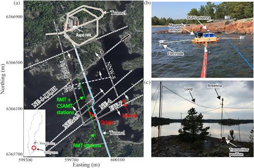
(a) Arial map of Äspö HRL area (Image © Google). The green dots are the CSAMT stations, and the transmitter to the east of the profile is indicated by a red star. A small island in the middle of the profile resulted in a gap in data acquisition. The origin of the coordinate system is marked by a red dot. (b) Boat-towed receiver system. The electric and magnetic field sensors were mounted on a floating platform together with a differential global positioning system (DGPS) antenna. The processing units, including the digitizer and computer system, and a palm computer for the DGPS, were inside the boat. (c) Two orthogonal horizontal magnetic dipoles used as the source to generate EM signals on an island.
5.2 Field data
The models computed from the RMT data set in our previous study (Wang et al.2018) motivated the use of the CSAMT method to better resolve the fracture zones below the 3–6 m deep brackish water at the Äspö HRL site. The locations of the controlled source and the CSAMT profile crossing these fracture zones are shown in Fig. 1(a) by a red star and green stars, respectively. The set-ups of the boat-towed receiver platform and the horizontal magnetic dipoles at the transmitter site are shown in Figs 1(b) and (c), respectively. Each transmitter loop has an area of about 27 m2 and a maximum dipole moment of 2700 Am2 is reached by using five loop windings and a maximum current of 20 A. The source was laid out on an island 310 m away from the nearest receiver station and 430 m away from the farthest one (Fig. 1a); thus the source position in the measurement coordinate system (see the origin in Fig. 1a) is x = −310 m, y = 0 m and z = 2.5 m (i.e. at 2.5 m above the sea level). Transmitter frequencies of 1.25, 2, 4, 6.25, 8, 10 and 12.5 kHz were chosen to guarantee the desired penetration depth of 30 to 50 m (based on Wang et al.2018). The transmitter was operated in two steps. In each step a single dipole in a given direction, y in our case, is active and sends a signal at a selected frequency. In the second step the other dipole (x direction) is active and the same frequency is transmitted. In step one only the scalar resistivity and phases are calculated. During the second stage, the other polarity is available and at the final part of the measurements the tensor results are inspected. The boat was moved along a rope that was fixed at both ends on land (Fig. 1b). The duration of CSAMT measurements is about 8 min per station, and the measurements are conducted with the boat stationary at each station. Use of the rope secured a stable measurement platform especially in slightly windy conditions. In total, 40 CSAMT stations and 40 collocated RMT stations along a 400-m long profile were collected within 2 d. Additionally, eight RMT stations were surveyed on land to estimate the resistivity of the granitic bedrock, which extended the whole profile to a length of 600 m. The apparent resistivities and phases derived from the Zxy and Zyx components of the impedance tensor field data are shown in Fig. 2. The location of the CSAMT profile does not coincide with the previous RMT profile in the study by Wang et al. (2018). This is a result of the rope being fixed to the island in the middle of the lake to achieve sufficient stability of the receiver system. The x-direction coincides with the geological strike direction estimated by Wang et al. (2018). The same strike direction is estimated in this study (see below) to within 5 to 8 deg. Hence, for the RMT data, the Zxy and Zyx impedances correspond to the TE and TM modes, respectively.
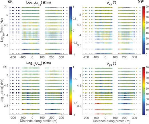
(a) RMT and CSAMT TE mode data, (b) RMT and CSAMT TM mode data. Left-hand and right-hand panels are apparent resistivity and phase, respectively. Low frequency data (<13 kHz) are collected using the controlled source. Crosses mark stations on land for which no controlled source data were acquired. Other removals, marked by crosses, indicate boat towed-data that had noise problems.
6 RESULTS
6.1 1-D inversion
For the CSAMT data, both distortion and source effects should be investigated before we invert the data using a routine 2-D inversion. We used the CSAMT and RMT 1-D modules of EMILIA (a package for 1-D and 2-D inversions for different EM methods; Kalscheuer et al.2008, 2010, 2012, 2015) that account for distortion and layer parameters and search for the simplest model. In the joint inversions of CSAMT and RMT data, this code uses separate sets of distortion parameters for each data set.
For 1-D inversion of the RMT and CSAMT data, we used an initial model with thirty layers of fixed thicknesses. The first layer was 0.5 m thick and layer thicknesses increased by a geometric progression factor of 1.2. The model resistivities and the distortion parameters of the data were simultaneously inverted for. All four elements of the impedance tensor shown in eq. (1) were used as inputs to the 1-D inversion. We tried inversions incorporating the VMTF (eq. 2) and the final models showed high data misfits. Therefore, the VMTF data were excluded from further consideration. The error floors of the impedance tensor elements were set to 5 per cent. Given that the complete impedance tensor was inverted, both the RMT and CSAMT responses show relatively reasonable data misfits at most stations in the 1-D inversions (Fig. 3) yielding average RMS values of 2.38 to 2.82. Note that the DOI (dashed white lines), following Spies’ (1989) method, show a lot of variability along the profile. The DOI is conservatively estimated as the skin depth, which is calculated for each station and accounting for the layering. At some stations, the DOI seems smaller than what one would expect. These small DOI values are caused by the shallow part of the respective models having very low resistivity. At −100–0 m distance along the profile, the stitched resistivity model from the CSAMT 1-D inversion models (Fig. 3b) resolves a resistor at about 20–40 m depth below the conductive water layer, whereas the model from the RMT 1-D inversion (Fig. 3a) does not show the same feature. This is because the CSAMT data have better resolution at greater depth than the RMT data. The 2-D stitched resistivity section (Fig. 3c) from the joint inversion of the full RMT and CSAMT impedance tensors combines the features from both single inversions. At 200–280 m along the profile, the conductive layer at 15–25 m depth in the RMT model is most likely caused by the fact that the RMT data are poorly explained by the model responses (cf. high RMS misfits at these stations in Fig. 3d). In Fig. 4, we show the impedance tensor elements of station 22 (marked in Fig. 3c) with the associated error bars and responses of the joint inversion model. The field data resemble a nearly 1-D plane-wave case where Zxx = Zyy = 0 and Zxy = −Zyx at about 35 per cent of all the stations.
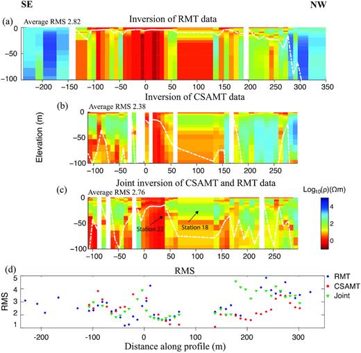
(a) Stitched resistivity model of RMT 1-D inversion results, average RMS of 48 individual inversions is 2.82. (b) Stitched resistivity model of CSAMT 1-D inversion results, average RMS of 40 individual inversions is 2.38. (c) Stitched resistivity model of the joint 1-D inversion results for the RMT and CSAMT data, average RMS of 40 individual inversions is 2.76 (land RMT stations were not used in the joint inversion). (d) RMS of the three inversions for each station. Empty station positions represent removed stations. The CSAMT data were inverted accounting for the source (Kalscheuer et al.2012). The white dashed lines in the models approximately represent the depth of investigation (DOI) estimated with the method proposed by Spies (1989). The land RMT stations are able to resolve the bedrock resistivity.
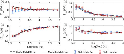
Measured and inversely modelled CSAMT and RMT impedances of station 22 indicated in Fig. 3(c): (a) Zxx, (b) Zxy, (c) Zyx and (d) Zyy. CSAMT data were inverted accounting for source (Kalscheuer et al.2012). RMS of CSAMT data is 1.53 and RMS of RMT data is 1.89. The diagonal elements of the impedance tensor are much smaller than the off-diagonal elements.
The estimated distortion parameters at station 22 are given in Table 1. The Pxx and Pyy values from the single inversion of CSAMT data and the joint inversion of RMT and CSAMT data have large absolute values, while the Pxx and Pyy values from the single inversion of RMT data show small values. Retrieving larger Ph values for the RMT data in the joint inversion indicates that the RMT and CSAMT data are not fully compatible in a 1-D sense and that 2-D or 3-D effects, that are not entirely obvious in the single inversions because of the disparate frequency ranges, are compensated for in the joint inversion by using larger Ph values for the RMT data. The Qh parameters of the CSAMT data are rather high, suggesting that some 2-D or 3-D induction effects are transformed into frequency-dependent distortion or that a certain degree of transmitter overprint (Zonge & Hughes 1991) exists even for purely inductively coupled sources. However, since transmitter overprint is predominantly a problem for galvano-inductively coupled sources (e.g. horizontal electric dipoles or long grounded cables), the former possibility of 2-D or 3-D induction effects being accommodated for by frequency-dependent distortion seems the more likely one. Since part of the distortion observed in the 1-D inversion seems to be caused by 2-D or 3-D geological structures at inductive scales, 2-D inversion is needed to further interpret the RMT and CSAMT data sets.
Distortion parameters for impedance tensor of station 22 from 1-D inversion: four elements for electrical field (Ph, no units) and four elements for magnetic field (Qh in A/V). The layered model is shown in Fig. 3.
| Parameter | Pxx | Pxy | Pyx | Pyy | Qxx | Qxy | Qyx | Qyy |
|---|---|---|---|---|---|---|---|---|
| CSAMT | −0.334 | 0.010 | 0.197 | −0.596 | −0.638 | 0.486 | 0.502 | 0.199 |
| RMT | −0.084 | −0.082 | 0.115 | −0.019 | 0.048 | −0.097 | 0.035 | 0.060 |
| Joint/CSAMT | −0.197 | 0.006 | 0.230 | −0.502 | −0.724 | 0.465 | 0.661 | 0.213 |
| Joint/RMT | −0.435 | −0.050 | 0.071 | −0.395 | 0.029 | −0.008 | −0.030 | 0.038 |
6.2 Analysis of CSAMT data for near-field effects
In order to model CSAMT data using a plane-wave approximation (PWA), the data need to be analysed for source effects, and data that do not fulfil the PWA need to be excluded before the inversion. The validity of the PWA depends on the transmitter–receiver distance relative to the plane-wave skin depth at a given transmitter frequency. A transmitter–receiver distance of at least five to ten times skin depth is needed to satisfy the PWA (Bartel & Jacobson 1987; Pedersen et al.2005). Using the resistivity model shown by Wang et al. (2018), the skin depth of the lowest transmission frequency (1.25 kHz) is about one tenth of the shortest transmitter–receiver distance, 310 m. However, Wannamaker (1997a,b) showed that a clear increase of resistivity at depth may require a distance between transmitter and receiver exceeding five to ten times the skin depth. Thus, care must be taken to use the PWA to invert the CSAMT data. In order to investigate the impedance and tipper at different transmitter–receiver distances for source effects, we resort to a comparative 1-D modelling study of plane-wave responses and CSAMT responses at different transmitter–receiver offsets using the 1-D model of station 18, which was recorded on shallow (<4 m deep) water and, thus, can be expected to show strong source effects. Fig. 5 clearly reveals that the phase of off-diagonal impedance and the imaginary part of tipper data have strong source effects at 1.25 kHz at 310 m away from the transmitter (corresponding to the closest receiver to the source in the field data). This influence on the transfer functions is larger than the noise levels assumed for the field data (deviations of 2.86 deg on phase and of 0.1 on tipper) until the transmitter–receiver distance increases to 400 m. Thus, the CSAMT data observed less than 400 m away from the transmitter at the frequency of 1.25 kHz were excluded in the subsequently presented inversions based on the PWA.
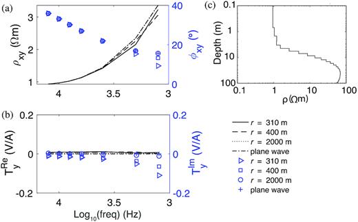
Comparison between the responses at different transmitter–receiver distances of 310, 400 and 2000 m and the plane-wave response, to study the near-field effects: (a) ρxy (lines) and ϕxy(symbols), (b) real part of Ty (lines) and its imaginary part (symbols) and (c) resistivity model from station 18 of the 1-D inversion (location in Fig. 3) used for the calculations. At the lowest frequencies, non-negligible near-field effects are observed both in the impedance phase and the imaginary part of Ty until the transmitter–receiver distance reaches 400 m. The other transfer function components are not shown since the model is 1-D.
6.3 Dimensionality, distortion and strike analysis
During the field measurements, the sensors were oriented parallel and perpendicular to the profile direction. Strike analysis of the RMT field data using the code by Zhang et al. (1987) shows that the preferred strike direction is about 82°–85° E with regard to the profile direction, that is, 74° East of geographic North, in a cumulative rose diagram (Fig. 6a). The estimated strike direction is approximately perpendicular to the profile direction. Swift skews (Swift 1967) of the most RMT data (Fig. 6b) are lower than 0.2, and only at one-third of the RMT sites and frequencies the Swift skews are larger than 0.2. These larger skew values were mostly observed in measurements that were performed close to a small island. Therefore, the RMT data can approximately represent a 2-D structure. Since the angular deviation between the estimated strike direction and the x-direction of our coordinate system is small, we have not applied further rotation to the coordinate system.
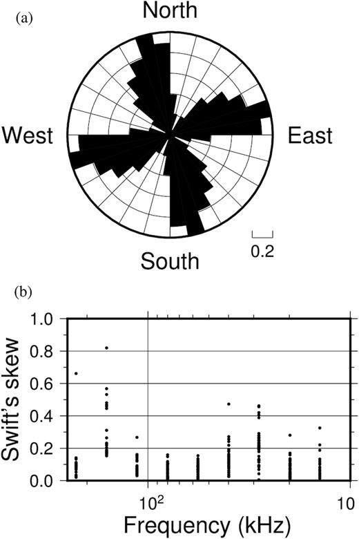
(a) Strike directions calculated with the method proposed by Zhang et al. (1987). The structure underneath the profile is 2-D with a preferred strike direction of 82° East with regard to the profile direction used in the field (corresponding to 74° East of geographic North). (b) Swift skews (Swift 1967). The underground structures along the profile are not perfectly 2-D, because the profile crossed an island in order to install a rope that enabled stable measurements on the water surface.
Note that Zhang et al. (1987) dimensionality, distortion and strike analysis cannot be applied to the CSAMT field data for two reasons. First, the analysis searches for a strike angle at which two real-valued distortion parameters relate the impedances in each column of the tensor to another, at least over a certain frequency band. However, in the transition and near-field zones of the source, Zxx and Zyy may differ from zero even in the undistorted 2-D case and, thus, may not be related to Zyx and Zxy, respectively, through simple real-valued distortion parameters. This holds even if the x axis is oriented along the strike. In rare cases, when the source is located on the profile, the symmetry of the set-up may suggest that MT strike analysis was applicable, but in our case this does not apply. Second, one may argue that MT strike analyses should be applicable at least for those CSAMT data which are recorded in the far-field zone of the source. Our 1-D inversion results (see above) contain relatively high values of Qh for the distortion of the magnetic field components. From the 1-D inversion results, it is not clear whether these high Qh are caused by 2-D or 3-D induction or are related to source overprint. Since the latter is not accounted for in Zhang et al. (1987) method and in most other dimensionality, distortion and strike analyses (e.g. Groom & Bailey 1989; McNeice & Jones 2001), we decided not to apply Zhang et al. (1987) analysis to the CSAMT data. For future strike analyses of far-field CSAMT data, it would be appropriate to use the method proposed by Chave & Torquil-Smith (1994), which takes distortion of both electric and magnetic fields into account.
6.4 2-D inversion based on plane-wave approximation
The first code we used to carry out 2-D inversion of the field data is EMILIA (Kalscheuer et al.2008, 2010) which inverts plane-wave data such as MT and RMT data. Using a plane-wave approximation to interpret CSAMT data has been reported previously (Boerner et al.1993; Wannamaker 1997a; Pedersen et al.2005; Bastani et al.2011; Shan et al.2016). For the 2-D inversion, EMILIA uses a finite-difference (FD) algorithm for forward modelling on a rectangular mesh. A Gauss–Newton (GN) algorithm is implemented with smoothness constraints. Thread-based parallelization of the numerical solver of the system of linear equations in the inverse problem and OpenMP parallelization over frequency of the forward response and sensitivity computations reduce the runtime.
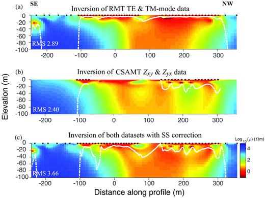
The field data analysis and the mesh generation for inverse modelling were carefully done to gain reasonable inversion results. Outliers in the RMT and CSAMT data were removed, because they violate the diffusive nature of EM fields (Ward & Hohmann 1988). Whether a data point can be considered an outlier partly depends on the error levels of the measurements. We excluded CSAMT data with near-field effects as described above. The same error floor as in 1-D inversion was applied in the 2-D inversion (i.e. 10 per cent in apparent resistivity and 2.86 deg for phase resulting from Gaussian error propagation and an assumption of 5 per cent relative error on the impedance tensor elements). The weights on horizontal and vertical smoothing were equal. A two-step inversion scheme was carried out: (1) Occam inversion using regular smoothness constraints; (2) Occam inversion with additional Marquardt–Levenberg damping, with the Lagrange multiplier for the Occam term selected as the one that gave the preferred model in step 1. The initial model in step 1 is a 100 ohm-m half-space model (this was used in all inversions), and the initial model in step 2 is the preferred model from step 1. The model mesh is finer at the station locations and the cell size gradually increases towards the edges of the mesh, until the mesh reaches an appropriate size for the Dirichlet boundary condition to be applied. Figs 7(a) and (b) show models from individual inversions of RMT and CSAMT TM mode data, where the input data were apparent resistivity and phase in either case. The white dashed line in the models presents the estimated DOI following Spies’ (1989) method for 1-D models with the layer parameters extracted from the vertical resistivity sections of the 2-D model at each station. We interpret the high-resistivity features in Figs 7(a) and (b) at both ends of the profile to correspond to the granitic bedrock. In Fig. 7(a), the conductive zone at 300 to 350 m distance and 5 to 50 m depth corresponds to the fracture zone NE-1 which is well documented and has also been delineated in our previous study (Wang et al.2018). At −240 to −150 m distance along the profile, two shallow (3–10 m depth) and moderately conductive (about 100 ohm-m) anomalies are observed. A warning for a high-voltage cable is visible at the site, but it is unclear whether there is any connection between the anomalies and the cable. The inversion of the CSAMT data resolves a rather vague conductive zone at 250 to 300 m distance and from 0 to about 50 m depth (Fig. 7b), which may correspond to the fracture zone EW-5 (Wikberg et al.1991; Wang et al.2018). However, the CSAMT single inversion model does not contain a conductive structure that would be interpreted as NE-1 due to the lack of data in that part of the model. The RMT model cannot resolve EW-5 due to the limited DOI. The inverted model using integrated RMT and CSAMT data (Fig. 7c) shows the combined features from both single inversions. Most notably, it indicates the presence of both NE-1 and EW-5.
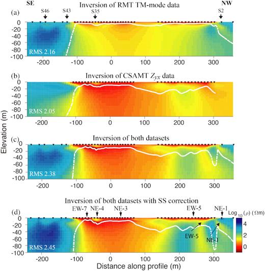
2-D inversion models for (a) RMT TM mode data, (b) CSAMT Zyx data, (c) RMT TM mode and CSAMT Zyx data and (d) RMT TM mode and CSAMT Zyx data with static shift (SS) correction. The black triangles on top of the models represent the receiver stations. The white dashed lines approximately represent the depth of investigation (DOI). All models were inverted using EMILIA with a plane-wave assumption (Kalscheuer et al.2008, 2010). Known information on fracture zones is marked on top of the model by arrows in Fig. 7(d).
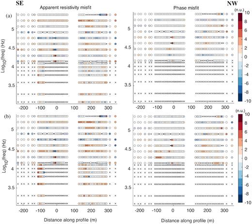
One does not normally observe galvanic distortions in marine EM data, because of the uniform resistivity of water. However, in our case, we have an island and shallow bathymetry along parts of the profile. Thus, a static shift correction was also applied in the inversion to improve the fit to data. The method of correcting static shift was as follows. An inversion was done with a 90 per cent error floor on apparent resistivity and 2.86 deg of phase error floor. Then, constant factors between the apparent resistivities of the inverted model and field data at each station were calculated from the two and were defined as static shift parameters (Fig. 8). Afterwards, these parameters were fixed in the inversion to correct for static shift (Siripunvaraporn & Egbert 2000). Fig. 7(d) shows the inversion results for RMT and CSAMT TM mode data with the static shift correction. The bedrock resistivity seems to be better determined, because it is known from Linde & Pedersen's (2004b) study that the granitic rock has a resistivity larger than 10 000 ohm-m at this site (Fig. 7d). Also, the transition between the north-western part of the lake and land at around 300 m distance along the profile is modelled more sharply. All the inversions have acceptable data misfits (RMS = 2.45 or less, Fig. 9). The crosses in (Fig. 9) indicate which data points were excluded in the inversions due to the lack of observations, insufficient quality or the near-field effect. The observation that the inversion models contain pronounced conductive zones in regions with known fractures seems to suggest that the distortion parameters obtained in the 1-D inversion are at least partly caused by the improper dimensionality. Single inversions of TE mode data and joint inversions of TE and TM mode data were also carried out to delineate resistivity structures and are shown in the Appendix.
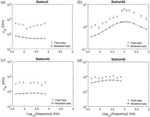
TM mode apparent resistivities of field data (blue) and of inverse model responses used for static-shift correction (black) at stations (a) 2, (b) 35, (c) 43 and (d) 46. The inversion was run with an error floor of 90 per cent on apparent resistivity to identify stations with static shift. The stations on land (e.g. Figs 8a, c and d) and a few stations on water (e.g. Fig. 8b) have obvious distortion, especially the stations on land. At station 35, a rock at roughly 1 m depth underneath the water surface seems to have caused the distortion. The selected stations are also marked in Fig. 7(a). The 2-D inversion model of the static shift corrected data is shown in Fig. 7(d).
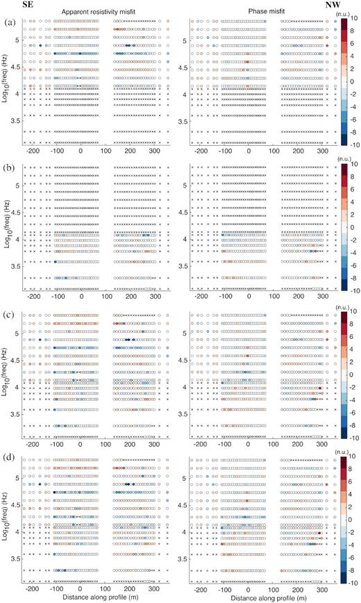
Normalized data misfits for the inversions, shown in Fig. 7, of (a) RMT TM mode data, (b) CSAMT Zyx data, (c) RMT TM mode and CSAMT Zyx data, and (d) RMT TM mode and CSAMT Zyx data with static shift correction. The misfits of apparent resistivity and phase are shown in the left-hand and right-hand panels, respectively. Crosses indicate data points that were not acquired or removed prior to inversion. The gap at 100 m distance corresponds to the position of the island.
The bedrock below the conductive water layer is not resolved at –100 to 50 m distance along the profile (Figs 7b–d) possibly due to the exclusion of the data at the lowest frequency. Therefore, an inversion code that incorporates source effects as well as the data at the lowest frequency is utilized to further study the CSAMT data.
6.5 2-D inversion incorporating source effects
6.5.1 Inversion code MARE2DEM
The second code used to conduct 2-D inversion of the boat-towed RMT and CSAMT data is MARE2DEM, which incorporates source effects to accurately model the CSAMT data. MARE2DEM is a publically available code for 2-D inversion of MT and CSEM data for onshore and offshore surveys (Key 2016). Unstructured grid parametrization in both forward and inverse modelling provides significantly better geometric flexibility and better computational efficiency than the structured rectangular grid used, for example, by EMILIA. A goal-oriented adaptive finite element method is implemented for the forward modelling (Li & Key 2007; Key & Ovall 2011; Key 2016). A dual-grid approach is used in MARE2DEM: a locally fine mesh at the receiver and source positions is generated automatically and refined by the error estimators in the forward modelling; a coarser mesh, generated by the code Mamba2D.m (Key 2016), is used for the inversion domain. The code is highly parallelized by partitioning the data into independent subsets consisting of a certain number of frequencies, transmitters and receivers (Key 2016). Each subset is separately modelled by an assigned computational unit under the coordination of message passing interface commands. The forward responses and sensitivities of all groups are then combined together in the iterative inversion that employs a Gauss–Newton method (de Groot-Hedlin & Constable 1990; Key 2016).
6.5.2 CSAMT modification of MARE2DEM
MARE2DEM uses different types of input data for 2-D inversions of MT and CSEM data. For example, the data may be linear or logarithmic apparent resistivities and phases for the MT method, and real and imaginary parts or amplitudes and phases of the electric and magnetic field components for the CSEM method. Neither CSAMT impedance tensors, as used in the previously presented 1-D and 2-D inversions of our field data, nor scalar CSAMT impedances are valid input data types in the current implementation of MARE2DEM. However, since the current of the transmitter was not recorded during our CSAMT data acquisition due to instrument limitations, the only data types of our field campaign suitable for inversion are the impedances (or VMTFs). In order to invert at least scalar CSAMT transfer function field data (our instrument stores both scalar and tensor transfer functions), a modification of MARE2DEM was required by implementing these data types in the input routines, output routines and the forward and sensitivity calculations. More specifically, in our modification, scalar transfer functions of type Zxy = Ex/Hy and Zyx = Ey/Hx are calculated from the EM signals of a single source as appropriate for a given source–receiver configuration. Moreover, in order to use MARE2DEM in the radiofrequency band (>1 kHz), 50 wavenumbers equally distributed from 10−5 to 101 m−1 in logarithmic space are used to reduce the source singularity based on scope and number tests for wavenumbers employed in the Fourier transformation along the strike direction. The tests are done with a total scope of 10−7 to 102 m−1 varying the number from 30 to 60. A source added at the right-hand side of the finite element equations results in an inaccurate solution for receiver positions close to the source. This is a disadvantage of modelling CSEM data using a total field approach (Mitsuhata et al. 2002) which is adopted in MARE2DEM. A magnetic dipole instead of a loop source is used for the CSAMT modelling, because the EM fields are measured at a distance of more than 50 loop diameters (around 5 m), which satisfies the condition for approximating a vertical transmitter loop by a horizontal magnetic dipole (Ward & Hohmann 1988).
A comparison between the semi-analytical solution calculated via CSAMT 1-D modelling and the numerical solution calculated via CSAMT 2-D modelling was done to verify our modification with a two-layered model. The top layer is 10 m thick and with 1.5 ohm-m resistivity underlain by a layer with 0.5 ohm-m resistivity. A horizontal magnetic dipole parallel to the x direction is used in the comparison. The signal frequencies and the positions of transmitter and receivers are the same as in the field campaign in order to better understand the field data. The semi-analytical and the numerical amplitudes and phases of the scalar impedances Zxy and Zyx as well as their relative errors (errors = (F1-D—F2-D)/F1-D, F represents either impedance amplitude or phase) are shown in Fig. 10. Both amplitude and phase of Zxy modelled by MARE2DEM show data differences in excess of 5 per cent for receivers at distance −70 to 70 m along profile direction (Figs 10a and b). Additionally, the impedance component Zyx shows a singularity at large distance at y ∼ 220 m (Figs 10c and d). According to Weitemeyer & Constable (2014), this additional singularity occurs within a certain azimuthal angle. Since these singularities affect the results from modelling the total field by MARE2DEM, we can only exclude CSAMT stations in the corresponding profile ranges with inaccurate 2-D solutions from further consideration in the subsequently presented 2-D inversion. The model chosen for this comparison resembles the situation in our field campaign with a layer of brackish water overlying more conductive lake-floor sediments. Varying the model, for instance, by including a third layer representative of resistive bedrock at depth, leads to changes in the responses. However, there is little variability in the profile ranges that need to be excluded from the subsequently presented 2-D inversion when the parameters of the 1-D model are changed within meaningful ranges.
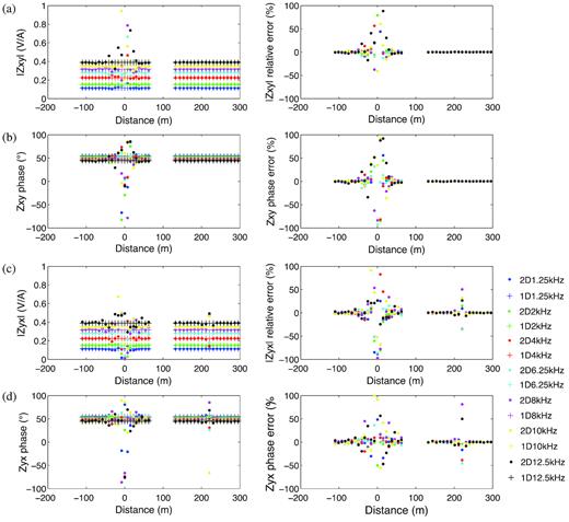
1-D semi-analytical and 2-D numerical solutions as well as their differences of (a) amplitudes of impedance Zxy, (b) phases of impedance Zxy, (c) amplitudes of impedance Zyx and (d) phases of impedance Zyx. Different frequencies are marked with different symbols. 2-D1.25 kHz represents the response at a signal frequency of 1.25 kHz calculated by MARE2DEM in 2-D. 1-D1.25 kHz represents the response at a signal frequency of 1.25 kHz calculated by EMILIA in 1-D. The source is located at (−310, 0, 2.5) m and the profile direction is y with x = 0 m and z = 0 m. Strong deviations between 1-D and 2-D solutions at y = −70 to 70 m led to exclusion of these field data in the subsequent 2-D inversions.
6.5.3 Synthetic test for inversion
A synthetic test was designed to show how well MARE2DEM can perform after the modification. A layered model shown in Fig. 11(a) was used for generating synthetic data. The top layer represents 10 m thick saline water with 1 ohm-m resistivity. It overlies a 20 m thick layer with 10 ohm-m resistivity. The third layer represents the bedrock with 1000 ohm-m resistivity. All of the receiver and transmitter positions as well as the frequencies are the same as in the field experiment (Fig. 1a). A magnetic dipole oriented in the x direction is used as a source, and it is located at 2.5 m above the surface to simulate the set-up used in the field. Due to the singularity of the source, receiver stations in the ranges of y = −70 to 70 m and at a distance of y ∼ 220 m were excluded from the simulations. The grids employed for forward modelling and inversion are very fine at the station and projected source locations, and coarser at the areas away from these locations. Five per cent Gaussian noise was added to the synthetic impedance data. A 100 ohm-m half-space model was used as an initial model in the subsequent inversions. The inversion results for the amplitude and phase data of the scalar impedances, Zxy and Zyx, are shown in Figs 11(b) and (c), respectively. The inversions resolve the top two layers of the true model underneath the parts of the profile that are covered by receivers (Figs 11b and c). The areas where we have no stations show very limited resolution. Therefore, these model regions should not be considered in the interpretation of the field data. Also, the result of the impedance Zyx shows slightly better resolution than the one for the impedance Zxy. This example demonstrates that the modification of MARE2DEM works sufficiently for the inversion of scalar CSAMT impedance data, and that the CSAMT signals can penetrate 30 m deep even in such an extreme case. The DOI evaluated by Spies's (1989) method (not shown here) approximately verifies that the top two layers in the synthetic model can be resolved.
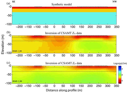
(a) Synthetic model, (b) 2-D inversion model for the data of CSAMT impedance Zxy, and (c) 2-D inversion model for the data of CSAMT impedance Zyx. The dashed lines represent the boundaries between different layers. Seven frequencies, 1.25, 2, 4, 6.25, 8, 10 and 12.5 kHz, were used in this synthetic test. Receivers are marked with triangles. A magnetic dipole oriented in the x direction is used as a source located at (−310, 0, 2.5) m and the profile direction is y. The synthetic data and inversion models were computed using MARE2DEM.
6.5.4 Inversion of field data
In accordance with the scalar CSAMT modelling approach implemented in MARE2DEM, we computed scalar CSAMT transfer functions from our field data. A 5 per cent error floor was used on the impedance data. A 100 ohm-m half-space model is used as an initial model. Note, that derivation of an initial model from the inversion model computed using EMILIA would require substantial effort in regridding the regular rectangular finite-difference mesh to an unstructured finite-element mesh. Hence, we have not tested this approach. The grid is very fine in the part of the initial model which contains the receivers. Towards the edges, the cell size increases to ascertain the validity of the employed Dirichlet boundary conditions and to avoid an unnecessarily high number of elements. In the forward modelling, the mesh was automatically refined based on error estimators (Ren et al.2013; Key 2016). Twelve receivers (i.e. all receivers after removal of those with inaccurate forward responses), one transmitter and all frequencies were grouped as one subset, meaning there were two subsets for CSAMT data and four subsets for RMT data.
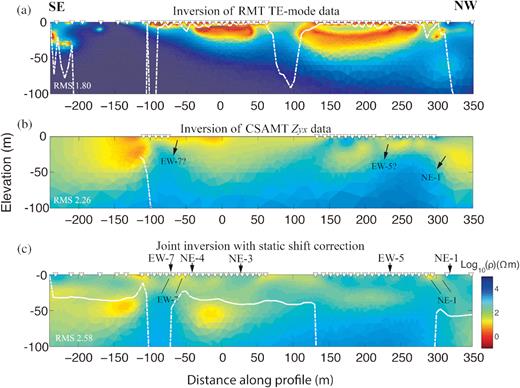
Both individual and joint inversions were used to mainly interpret the boat-towed RMT TM-mode data and CSAMT Zyx data (CSAMT data cannot be simply identified as TE or TM mode outside the far-field zone), because TM-mode data show better resolution for the delineation of fracture zones than TE-mode data (Figs 7 and A1). In our particular case, 2-D inversion of TM-mode data seems preferable, because the TE-mode data are more sensitive to 3-D structure and they are more affected by a finite-water depth than TM-mode data (Andreis & MacGregor 2007). Note that a joint inversion of CSAMT TM-mode and TE-mode data resulted in poor convergence, and the results are not shown here. In order to reduce the potential artefacts caused by smoothing in the vertical direction in our model, three times more smoothing weight in the horizontal direction was applied in all inversion models. Note that the differences in gridding in the 2-D inversion codes used in this study (regular finite-difference grid in EMILIA versus unstructured finite-element grid in MARE2DEM) require largely different weights on horizontal and vertical smoothing to be used. The inverse model for logarithmic apparent resistivities and phases of the RMT TM-mode data is shown in Fig. 12(a). The conductive zone, corresponding to the fracture zone NE-1, is resolved at around 300 to 350 m distance along the profile. Below the lake bottom, conductive zones along the profile may be artefacts due to the limited penetration depth of the RMT signals. The inverse model for the CSAMT Zyx impedance data is shown in Fig. 12(b). The data are logarithmic amplitudes of the CSAMT impedance Zyx from the measurements with the loop which is parallel to the profile (the phase data are of low quality probably due to an insufficient number of measurement stacks). The data from the perpendicular loop have low quality due to the faster decay of the fields, so we excluded them. Due to the source singularity in the code, the closest stations to the transmitter as well as the ones at a distance of about 220 m along the profile were excluded in the inversion. One conductive zone is shown in Fig. 12(b) at distances of 300 to 350 m along the profile, which may be NE-1. For the other speculative conductive fracture zones, no supportive evidence is available in Fig. 12(b).
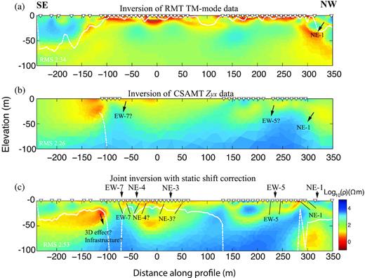
2-D inversion models computed using MARE2DEM with a finite-element mesh. (a) single inversion model for RMT TM-mode data, (b) single inversion model for CSAMT impedance Zyx data and (c) joint inversion model for both data sets with five times more weight on CSAMT data set and with static shift correction. The triangles mark receiver positions. The white dashed lines approximately represent the depth of investigation (DOI). Some model regions, such as in (b), are without white line, because there is a lack of stations or the DOI values are larger than 100 m. Geological and borehole information are marked with arrows at the top of the model in (c).
Joint inversion of RMT and CSAMT with the static shift correction is shown in Fig. 12(c). Five times more weight on the CSAMT data set than on the RMT data set was used for the inversion, because there are fewer CSAMT stations than RMT stations and the CSAMT data have better resolution at depth (Figs 12a and b). In the joint inversion model (Fig. 12c), the conductive zones are obviously better resolved than in any single inversion (Figs 12a and b). Based on a comparison to the existing geological, limited borehole and low-resolution geophysical information marked by arrows above the surface (cf. Figs 1a and 7d), we interpret the fracture zones NE-1, EW-5 and EW-7 to be partly resolved. However, the tentatively interpreted conductive zones NE-3 and NE-4 in the joint inversion model need to be further studied, even though their positions match well with the prior information. The conductive zone at around −150 to −100 m distance along the profile (Figs 12a–c) was not observed in the 2-D inversion models computed using EMILIA (Fig. 7). Hence, this conductor may be an artefact of smoothing in MARE2DEM, and, for the CSAMT data, its pronounced spread towards the southeast may be caused by a shadow-zone effect of the source (Boschetto & Hohmann 1991; Zonge & Hughes 1991). All the inversions have acceptable data misfits (RMS = 2.53 or less; Fig. 13). The single and joint inversion models of the RMT TE-mode data and the CSAMT Zyx impedance data are shown in the Appendix.
(a) The normalized data misfits of the RMT TM-mode apparent resistivity, RMT TM-mode phase and amplitude of CSAMT impedance Zyx for single inversion models in Figs 12(a) and (b). (b) The data misfits of RMT TM-mode apparent resistivity, RMT TM-mode phase and amplitude of CSAMT impedance Zyx for joint inversion model in Fig. 12(c).
6.6 Evaluation of inversions
Further evaluation of the reliability of our inversion results is required. Particularly, the resolution in some parts of the inversion models may be limited by the conductive water. Looking at the data misfit is a way to evaluate the inversions. In our inversions, reasonable RMS values and well-distributed misfits are obtained (Figs 9 and 13). Total sensitivities calculated by the method of Schwalenberg et al. (2002) based on the inverted models (Fig. 12) illustrate that the joint inversion potentially improves the resolution at depth compared with the single inversions (Fig. 14). This is so, because the joint inversion combines the sensitivities of the RMT and CSAMT data. Furthermore, using MARE2DEM, we carried out a synthetic test based on the joint inversion results to evaluate the resolution of the boat-towed RMT and CSAMT data. The single inversion models were not used, since the joint inversion model shows all the important information. Fracture zones and other structures that agree with previous geological knowledge together with other speculated fracture zones in the joint inversion model (Fig. 12c) were introduced into a synthetic model (Fig. 15a). The model has the resistivities of water, fracture zones and bedrock set to 1.5, 10 and 10 000 ohm-m, respectively. Synthetic RMT and CSAMT data were then generated using the same acquisition parameters as in the edited field data sets in Fig. 12. To simulate the noise level of the field data, 5 per cent Gaussian noise on the impedances was added to the synthetic data. Single and joint inversions of logarithmic apparent resistivities and phases of the RMT TM mode data and logarithmic amplitudes of the CSAMT impedance Zyx data were carried out. The single inversion of the RMT data (Fig. 15b) shows poorer resolution at depth than the single inversion of the CSAMT data (Fig. 15c) due to the limited DOI of the RMT signals. Joint inversion of RMT and CSAMT data resolves some of the low-resistivity fracture zones underneath those parts of the profile covered by both data sets, especially for the presumed fracture zones NE-1, EW-5 and EW-7 in the upper 20 m (Fig. 15d). However, the fracture zones NE3 and NE4 are not distinguished in the model. The synthetic test indicates that the interpretation of the field data sets is to a certain degree reasonable. The structure at the bottom of and underneath the conductive sea water is uncertain for two reasons: (1) lack of sensitivity that is basically due to the limited penetration depth and (2) EM methods are known to perform poorly at resolving structures at the bottom of or immediately below low-resistivity features (Bedrosian 2007; Kalscheuer et al.2018). In spite of this, the true resistivity of the bedrock in the synthetic test is resolved in the joint inversion, mostly owing to the use of RMT stations on land and the greater penetration depth of the CSAMT signal underneath the lake floor.
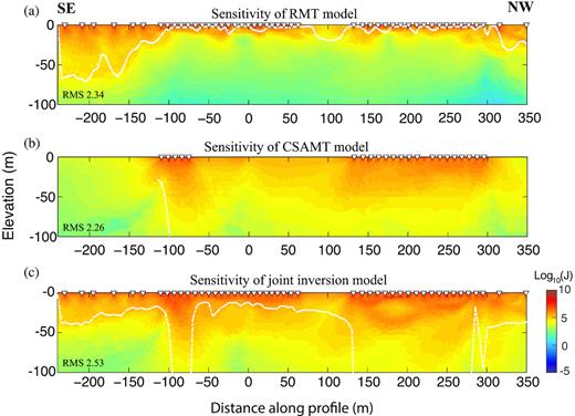
2-D total sensitivities calculated for the models in Fig. 12, (a) RMT model, (b) CSAMT model and (c) joint inversion model. Total sensitivities were computed as sums over all data points of the absolute values of sensitivities normalized by data uncertainty and cell area following Schwalenberg et al. (2002). The triangles mark receiver positions. The white dashed lines approximately represent the depth of investigation (DOI). In general, sensitivity decreases with increasing depth. In the deeper parts of the model with CSAMT coverage, the sensitivity values of the CSAMT data are higher than those of the RMT data.
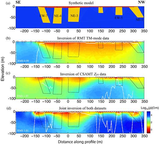
(a) 2-D model deduced from the 2-D joint inversion model shown in Fig. 12(c), (b) 2-D inversion model for synthetic RMT TM-mode data, (c) 2-D inversion model for synthetic CSAMT Zyx data and (d) 2-D joint inversion model for both data sets with five times more weight on CSAMT data set. The black dashed lines mark the positions of fracture zones. The white dashed lines approximately represent the depth of investigation (DOI). The inverse triangles are receiver positions, the source position is (−310, 0, 2.5) m and the profile direction is y. Targets which are not covered by both data sets are not well reconstructed, such as NE-3 and NE-4.
7 DISCUSSIONS
7.1 High efficiency in data acquisition
We employed a boat-towed CSAMT method for the first time for resolving conductive fracture zones below a lake at the Äspö HRL site as a continuation of our previous study (Wang et al.2018), which itself followed the earlier successful use of boat-towed RMT (Bastani et al.2015; Mehta et al.2017). The field data acquisition follows a highly efficient workflow. A 400-m-long boat-towed CSAMT profile together with a collocated RMT profile with 10 m station spacing was easily surveyed within 2 d, eradicating the need for instrument transportation in the field which is usually the heaviest work in the MT and RMT data acquisition on land. Moreover, this method has better penetration depth than the boat-towed RMT method due to the utilization of the controlled source for lower frequency signals (Bastani 2001; Wang et al.2017). Thus, the boat-towed CSAMT method guarantees that the data acquisition is suitable for detailed 2-D and 3-D surveys and to resolve relatively deep and complex subsurface structures up to very roughly 50 and 20 m depth underneath shallow fresh water and saline water bodies, respectively. This ability is important for underwater infrastructure planning, since other resistivity-based methods, such as ERT and boat-towed RMT, hardly show comparable acquisition efficiency, resolution and deployment efficiency simultaneously. Particularly, once the transmitter deployment is done, multiple profiles can be easily surveyed. Note that boat-towed transient electromagnetic methods (Barrett et al.2005; Hatch et al.2010; Mollidor et al.2013; Bekesi et al.2014) have similar acquisition efficiency and penetration depth, but do not offer multicomponent measurements and dual source polarizations.
7.2 1-D and 2-D inversions of CSAMT data
Two available tools, EMILIA and MARE2DEM, were used to invert the boat-towed CSAMT and RMT data. The distortion parameters resolved by the 1-D inversion in EMILIA suggested using 2-D inversion to model the data, which is also compatible with what we observed in the previous study (Wang et al.2018). The approximate inversion of the CSAMT data based on the PWA shows better resolution at depth than the inversion of the RMT data due to the enhanced DOI (Figs 7a and b). This strongly demonstrates the advantage of the boat-towed CSAMT method compared to the boat-towed RMT method in such an environment. Single 2-D inversions of RMT and CSAMT data resolve the fracture zones NE-1 and EW-5, respectively, and therefore the inversion of the integrated data sets simultaneously resolves both fracture zones (Fig. 7). The traditional way of inverting CSAMT data using a PWA should be considered with care, even though the approximation seems reasonable when the transmitter–receiver distance is 5–10 times larger than the skin depth (Bartel & Jacobson 1987; Pedersen et al.2005). A careful analysis shown in Fig. 5 based on 1-D CSAMT forward modelling also proves this. Thus, the signals at the lowest frequency in our data set were excluded in the inversion using the PWA to avoid any misleading results. One should remember that simply using the ratio of a source–receiver distance to skin depth based on certain information is not enough to indicate the existence of the near-field effect, especially when the geology is complicated.
Since the source current is not recorded by the data acquisition system, inversion of individual field components, as supported by MARE2DEM, was not possible. Hence, we modified MARE2DEM to invert CSAMT scalar impedances, adding the relevant modifications to the forward modelling and sensitivity calculations. Both forward and inverse modelling based on a conceptual layered model show that our modification for MARE2DEM is reasonable and accurate. This is the first time that MARE2DEM has been used to invert radiofrequency signals. The inversion of the scalar CSAMT field data using the modified MARE2DEM code shows reasonable resolution (Fig. 12b). Moreover, the CSAMT data contain more information of underwater structures but have fewer data points than the RMT data, so that using five times more weight on the CSAMT data set in the joint inversion was imposed to delineate structures at depth. The resulting joint inversion model in Fig. 12(c) seems to indicate the conductive fracture zones NE-1, EW-5 and EW-7. Owing to the pronounced source singularity and the ensuing numeric difficulties in modelling the source, almost half of the CSAMT stations had to be excluded from the 2-D inversions using MARE2DEM.
7.3 Resolution evaluation
Resolution analysis is an important step to know how reliable inversion results are. In our case, the model resolution provided by the field data is limited by the saline water at the surface. Three steps were taken for evaluation. In the first step, data misfits and exploration depth are evaluated (Figs 7, 9, 12 and 13). Reasonable misfits should be obtained in the inversions. Exploration depth combined with data coverage can indicate which part of the model could be reliable. In the second step, total sensitivities were used to check the improvement obtained using joint inversion as well as potentially reliable structures in the joint inversion model. In the third step, a synthetic test based on the resolved structures was done, to study which structures in the model are reliable (Fig. 15). The synthetic test with a layered structure in Fig. 11 shows that the CSAMT method can resolve the basement at up to 30 m depth, even though 10 m thick saline water with 1 ohm-m resistivity, that is, with a lower resistivity than observed by in situ measurements, was located at the top part of the model. Considering Fig. 15, the presumed fracture zones NE-1, EW-5 and EW-7 are well constrained at shallow depth by the combination of RMT and CSAMT. The conductive zones marked as NE-3 and NE-4 in Fig. 12(c) are not reliable based on the synthetic test and need further study.
7.4 Future improvements
Both modelling and instrumental aspects of the CSAMT method need improvement. First, in the field example presented here, almost half of the CSAMT stations had to be excluded from the inversions using MARE2DEM because of the inaccurate modelling results in a range of −70 to 70 m along the profile. This suggests that further improvement to MARE2DEM for land CSEM surveys is highly desirable when the source and receivers are not along the same profile. Second, we would want to implement the inversion of tensor transfer functions in MARE2DEM. This would offer a better possibility to compare the models to those from 1-D and 2-D inversions by EMILIA which use the full tensor and the off-diagonal elements of the impedance tensor, respectively. However, when compared to the first point, this improvement may be of lower importance. Third, the current generated by the source during the data acquisition should be recorded, and then the controlled source EM fields could be inverted directly. Inverting for a resistivity model using EM field components as input data rather than transfer functions may provide more detailed information of the subsurface. However, modelling studies are required for verification. These three modifications can further improve the resolution capability of CSAMT data for targets underneath conductive shallow water bodies and conductive overburden in general.
8 CONCLUSIONS
The implementation of the boat-towed CSAMT method is a new achievement after the boat-towed RMT method was successfully utilized for modelling structures below water bodies and specifically in the delineation of fracture zones. The new approach, used in fracture zone mapping at Äspö HRL, demonstrates high efficiency in data acquisition. An inversion code tuned to the dimensionality of the problem can be expected to provide more reasonable details in the resulting inversion models. Using 2-D inversions of the RMT and CSAMT data, we can resolve fracture zones at depth. Especially, the 2-D joint inversion of boat-towed RMT and CSAMT, which was implemented here for the first time, shows better resolution for the fracture zones than single inversions. For further improvements, the present boat-towed CSAMT system needs to be upgraded to record the source current.
The 2-D inversion of CSAMT data using MARE2DEM carries the promise of improved utilization of CSAMT data for mapping fracture zones compared with using a plane-wave approximation. Proper modelling of CSAMT data with due regard for the source allows inclusion of low-frequency data which otherwise have to be excluded in a plane-wave approach. However, the numerical inaccuracies in the MARE2DEM forward modelling results close to the source suggest that the modelling scheme needs improvement when the source and receivers are not along the same profile. With the current implementation of MARE2DEM and for our field data set, almost half of the CSAMT stations had to be excluded from the inversion.
The boat-towed CSAMT method can play an effective role in geo-engineering studies. The improved acquisition efficiency can reduce the planning costs of underwater construction. Moreover, the improved resolution of subsurface models provided by joint inversion of boat-towed RMT and CSAMT data can help geo-engineers to identify fracture or weak zones in bedrock underneath shallow water. The new method is cost-effective and can be successfully applied in countries such as Sweden, Norway and Finland that are largely covered by shallow waterbodies. This extends the application field for the traditional CSAMT method. Certainly, the method is not restricted to geo-engineering applications, and it can also be introduced in geohazard investigations and underwater mineral explorations.
ACKNOWLEDGEMENTS
This work was carried out within the frame of the TRUST (http://trust-geoinfra.se) project sponsored by Formas, SGU, SKB, Nova, BeFo, SBUF/Skanska, FQM and NGI. SKB is thanked for providing access to the site and provided support for the measurements. Nova is thanked for partly funding this work. Laust B. Pedersen is sincerely appreciated for constructive discussions and will be sorely missed. We thank S. Mehta for his field contribution and L. Dynesius for the equipment preparation. K. Key and C. Gustafson are thanked for helpful discussions. SW thanks the China Scholarship Council (201306370039), Formas (25220121907), National Natural Science Foundation of China (41227803) and Byzantine travel scholarship for supporting his PhD study at Uppsala University and at Scripps Institution of Oceanography (SIO), and the Cecil & Ida Green Foundation and the Seafloor Electromagnetic Methods Consortium at SIO for postdoctoral support. Dr Arseny Shlykov, one anonymous reviewer and the editor Ute Weckmann are thanked for their helpful and constructive comments on the manuscript.
REFERENCES
APPENDIX
Inversions of the RMT TE-mode and CSAMT Zxy data were also carried out using EMILIA. All the inversion settings such as the initial model, the finite-difference mesh and the weights on horizontal and vertical smoothing were the same as those for the RMT TM-mode and CSAMT Zyx data shown in the main text. The inversion models in Fig. A1 show limited information about the conductive zones compared with the inversions for RMT TM-mode and CSAMT Zyx data (Fig. 7), except for an anomaly at −240 to −200 m distance along the profile. RMT TE-mode and CSAMT Zxy data have poorer lateral resolution compared with RMT TM-mode and CSAMT Zyx data. This is so, because RMT TE-mode and CSAMT Zxy data are more sensitive to 3-D structure (Berdichevsky et al.1998). The joint inversion results for RMT TE-mode and TM-mode data, CSAMT Zxy and Zyx data and the combination of all four data sets are shown in Fig. A2. They contain fewer distinct structures than observed in the inversions of RMT TM-mode and CSAMT Zyx data, and the data misfits are also larger than for inversions of single mode data (Fig. A2). This is probably because the data of the two modes are sensitive to different aspects of the subsurface structures. However, the inversion models of the TM-mode data show higher resolution than the TE-mode data.
2-D inversion models for (a) RMT TE-mode data, (b) CSAMT Zxy data and (c) RMT TE-mode and CSAMT Zxy data with static shift correction. The black triangles at the surface represent station positions. The white dashed lines approximately represent the depth of investigation (DOI). All models were computed using EMILIA, and a plane-wave assumption was used for CSAMT data.
2-D inversion models for (a) RMT TE-mode and TM-mode data, (b) CSAMT Zxy and Zyx data and (c) RMT TE-mode, RMT TM-mode, CSAMT Zxy and CSAMT Zyx data with static shift correction. The black triangles at the surface represent station positions. The white dashed lines approximately represent the depth of investigation (DOI). All models were computed using EMILIA and a plane-wave assumption is used for CSAMT data.
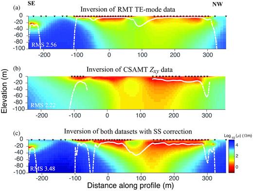
The single inversion of the RMT TE-mode data and the joint inversion of the RMT TE-mode and CSAMT Zyx data were also carried out using MARE2DEM. All the inversion settings were the same as those for the RMT TM-mode data in the main text, such as the initial model, the mesh used for forward and inverse modelling, weighting of data sets and weighting of model smoothness in different directions. The inversion model of the RMT TE-mode data set is shown in Fig. A3(a). The fracture zone NE-1 is unclear at around 300 m distance along the profile. The inversion for CSAMT Zxy impedance data did not converge, thus the CSAMT Zyx impedance data is shown again (Fig. A3b) and used for the joint inversion. Joint inversion with five times more weight on CSAMT data than on RMT data with static shift correction was used to compute inversion models (Fig. A3c). The known subsurface structures (fracture zones NE-1, EW-5 and EW-7) in the joint inversion model are obviously as poorly resolved as in the single inversions (Figs A3a and b).
(a) 2-D inversion model for RMT TE-mode data, (b) 2-D inversion model for CSAMT impedance Zyx data, (c) 2-D joint inversion model for both data sets with five times more weight on CSAMT data and with static shift correction. The inverse triangles mark receiver positions. The white dashed lines approximately represent the depth of investigation (DOI). The source is at (−310, 0, 2.5) m position and the profile direction is y. All models were computed using MARE2DEM. The geological and borehole information are marked with arrows at the top of the model in (c).
