


SUMMARY
On 2012 August 11, an earthquake doublet (Mw6.5 and Mw6.3), separated in time by 11 min, occur in the northwest of Iran. The hypocentres of these earthquakes are close (∼6 km) and located near the cities of Ahar and Varzaghan. The rupture process of both main shocks is retrieved by inverting the near-field strong motions data and using the elliptical subfault approximation method. Our calculations show that the two earthquakes are occurring on two distinct fault planes: the first main shock (M1) has nucleated at a depth of ∼8.5 km, and is located ∼4 km east of the eastern termination of the E-W trending surface rupture. The slip reaches the ground surface west of the hypocentre on an E-W striking fault (N88°E) that dips almost vertically (80°S). This earthquake exhibits a right-lateral strike-slip mechanism. The entire slip is imaged on a single patch that ruptures with an average speed of 2.4 km s−1. The rupture duration is ∼5.6 s and the earthquake releases a seismic moment of ∼8.41E + 18 N·m. The slip reaches the surface with a right-lateral dislocation value of ∼1 m, which is consistent with the observed surface rupture. About 11 min later, the second main shock (M2) nucleates ∼5 km to the west and 4 km to the north with respect to the hypocentre of the M1, and at a depth of ∼16.5 km. The M2 rupture evolves toward shallower depths and to the west on an ENE-WSW oriented fault plane (strike ∼256°) with a dip of ∼60° northward. The slip is essentially distributed on two distinct patches with strike-slip and reverse mechanisms, respectively. The first patch has a pure right-lateral strike-slip mechanism, and ruptures at a relatively fast speed of over 2.8 km s−1, and last for about 2.6 s until it reaches the second patch. The latter has a reverse mechanism (rake∼112°) and extends the rupture toward shallow depths, and to the west at a speed of ∼2.5 km s−1, and its rupture lasts for ∼2.5 s. The top of the slip distribution of M2 stops at a depth of ∼8 km. We observe that aftershocks surround the M1 and most of the M2 slip models. They are not distributed in the region of high slip (∼3.1 m) of M1. We show that the rupture of M2 is controlled by the static Coulomb stress changes caused by M1, with the maximum slip of M2 located in the positive Coulomb stress caused by M1. The M2 rupture stops where it reaches the area of high negative Coulomb stress change (over −10 bars). The cumulative Coulomb stress fields of both main shocks show a transfer of positive static Coulomb stress change of >0.1 bars on the eastern segment of the North Tabriz Fault. This segment did not rupture since the 1721 M∼7.6–7.7 event that has destroyed the city of Tabriz, and that currently hosts 2 million people. The occurrence of this earthquake doublet with different mechanisms reveals the slip partitioning of the oblique convergence regime of NW Iran on the Ahar–Varzaghan complex fault system.
1 INTRODUCTION
Earthquake doublets are two earthquakes with comparable magnitudes that are close in time and space. They can occur in different segments of the same fault or on two different faults (e.g. Lay & Kanamori 1980; Toda & Stein 2003). They are often located in complex fault systems which favour stress interactions (e.g. Lay & Kanamori 1980; Kagan & Jackson 1999; Vallee & Di Luccio 2005; Ammon et al. 2008; Lay et al. 2010; Nakano et al. 2010; Nissen et al. 2016; Ye et al. 2016).
On 2012 August 11, two shallow destructive earthquakes (Mw6.5 and Mw6.3; hereafter referred to as M1 and M2, respectively) occur close to the cities of Ahar and Varzaghan, northwest of Iran and have caused over 300 fatalities and 3000 injuries (Razzaghi & Ghafory-Ashtiany 2012). The peak ground acceleration of M1 and M2 is 0.48g and 0.53g, respectively. Both earthquakes are close in space (∼6 km) and time (∼11 min). In terms of mechanism, M1 exhibits an almost pure strike-slip faulting, while M2 is a reverse faulting earthquake with a significant strike-slip component (Fig. 1). Field observations reveal 12–13 km of surface ruptures (Faridi & Sartibi 2012) striking E-W with dominant right-lateral strike-slip faulting, and with up to ∼1 m of horizontal offset and ∼20 cm of uplift of the southern block on the western part of the rupture (Fig. 1).
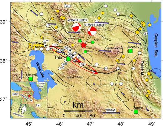
Map of the tectonic context of the study area. Stars are the Ahar–Varzaghan earthquake doublet (M1 12:23:16 GMT and M2 12:34:34 GMT) with the respective focal mechanisms (Momeni & Tatar 2018). Big squares are large cities (>500 000 people) and small squares are small cities (∼100 000 people) close to the 2012 doublet earthquake. Hexagons are historical earthquakes (M > 6.5) from Ambraseys & Melville (1982) catalogue. Circles are instrumental earthquakes (5 < M < 6.1) from Engdahl et al. (2006) catalogue. Solid lines are active faults (Faridi 2013). Vectors show GPS velocities relative to fixed central Iran (Masson et al. 2006). NTF stands for the well-known North Tabriz Fault. The two ellipses represent the surface ruptures related to the M7.6–7.7 1721 and M7.4 1780 historical earthquakes.
The Ahar–Varzaghan earthquake doublet has occurred on previously unrecognized faults within a zone of right-lateral strike-slip faulting in the Turkish-Iranian plateau (Fig. 1). This region mostly accommodates the strike-slip component of the Arabia-Eurasia oblique convergence relative motion (Jackson 1992; Copley & Jackson 2006) as also evidenced by GPS (Global Positioning System) measurements (Vernant et al. 2004; Masson et al. 2006; Reilinger et al. 2006; Djamour et al. 2011).
These earthquakes are the only well-recorded (>100 seismic stations within a 300 km radius from the epicentres) large seismic events (M > 6) in NW Iran, north of the well-known North Tabriz Fault (NTF), which stretches over 500 km and crosses the northern part of the city of Tabriz with a population of over two million (Fig. 1). Indeed, prior to this doublet, the instrumental seismic activity recorded by the Iranian permanent National Seismic network of the Iranian Seismological Center (IRSC) in the Ahar–Varzaghan region was negligible (Momeni & Tatar 2018). The last major historical earthquakes that have occurred on the NTF are the 1780 magnitude 7.4 and 1721 magnitude 7.6–7.7 events (Ambraseys & Melville 1982; Berberian 1994; Berberian 1997) both showing ∼50 km of surface ruptures (red ellipses on Fig. 1) and causing over 200 000 fatalities in the city of Tabriz. Recent GPS measurements on the NTF showed ∼7 mm yr−1 of right lateral surface deformation (Djamour et al. 2011).
Recent microseismic activity on NTF monitored by a local temporary seismic network confirms the right-lateral strike-slip mechanism along east–southeast trending fault planes (Moradi et al. 2011). The occurrence of the earthquake doublet 50 km north of the NTF highlights the presence of a previously unidentified and complex fault system and indicates spatially distributed deformation in this region. Studying the rupture kinematics of the Ahar–Varzaghan earthquake doublet is important for better understanding the complexity of the interactions between faults at the local scale as well as their interactions with the NTF at a larger scale. The ultimate goal is the assessment of the earthquake hazard and the understanding of the recent tectonics in this high-risk area.
2 UNCERTAINTIES ON THE LOCALIZATION AND GEOMETRY OF THE MAIN SHOCKS RUPTURES
Previous studies based on seismology, InSAR and field observations reach different conclusions on the localization and rupture geometry of these two main events (Alipour 2013; Copley et al. 2013; Donner et al. 2015; Ghods et al. 2015; Zafarani et al. 2015; Rezapour 2016; Yadav et al. 2016; Amini et al. 2018; Momeni & Tatar 2018; Yazdi et al. 2018; see Table 1). Most of them agree on the EW strike of M1, while there is no agreement on its dip and the strike and dip of the M2 fault plane.
Location and geometry of the M1 and M2 ruptures reported by previous studies.
| Hypocentre | Centroid | |||||||||
|---|---|---|---|---|---|---|---|---|---|---|
| Study | Main shock | Data | Method | Lat. (°N) | Lon. (°E) | Depth (km) | Lat. (°N) | Lon. (°E) | Depth (km) | Fault geometry Strike/dip/rake (°) |
| Alipour (2013) | M1 | Radarsat2 | INSAR | – | – | 268/90/- | ||||
| M2 | – | – | 268/90/- | |||||||
| Donner et al. (2015) | M1 | Seismic (IRSC&BIN& IRIS) | Moment tensor inversion | – | 38.399 | 46.842 | 6 | 265/45/166 | ||
| M2 | – | 38.425 | 46.777 | 12 | NNE/ESE/-(argued) | |||||
| Ghods et al. (2015) | M1 | Seismic (IRSC&BIN&IRIS) | Seismotectonic investigation | 38.399 | 46.842 | 14 | – | E-W/70/- | ||
| M2 | 38.425 | 46.777 | 17 | – | ENE-WSW/70/- | |||||
| Zafarani et al. (2015) | M1 | Strong motions (ISMN) | Stochastic source simulation | – | 38.31 | 46.80 | 15 | 84/84/170 (GCMT-fixed) | ||
| M2 | – | 38.35 | 46.78 | 19.2 | 255/63/134 (GCMT-fixed) | |||||
| Yadav et al. (2016) | M1 | GPS (NCI) | Slip inversion | – | – | 265/90/- | ||||
| M2 | – | – | ∼N/ESE/- | |||||||
| Rezapour (2016) | M1 | Seismic (IRSC&BIN) | Seismotectonic investigation | 38.436 | 46.838 | 16.4 | – | ∼E-W/70/- | ||
| M2 | 38.416 | 46.815 | 15.4 | – | ∼ENE-WSW/70/- | |||||
| Yazdi et al. (2018) | M1 | Seismic (IRSC&BIN) | Seismotectonic investigation | 38.425 | 46.825 | 10 | – | 268/90/- (GCMT) | ||
| M2 | Stress modelling | 38.395 | 46.805 | 10 | – | ∼N/∼ESE/- (GCMT) | ||||
| Amini et al. (2018) | M1 | Seismic (Teleseismic& IRSC) | Source inversion, Stress modelling | 38.40 | 46.84 | 12 | – | 88/90/- (posed) | ||
| M2 | – | – | 10/50/36 (GCMT fixed) | |||||||
| Momeni & Tatar (2018) | M1 | Seismic (Local network& IRSC& BIN& IRIS) | Seismotectonic investigation, Moment tensor inversion | 38.395 | 46.83 | 10 | 38.39 | 46.87 | 5 | 266/87/-148 |
| M2 | 38.43 | 46.80 | 15 | 38.42 | 46.75 | 11 | 261/71/132 | |||
Alipour (2013) has measured the coseismic (along with some post-seismic) surface deformation of the doublet using RADARSAT2 satellite images. She concludes that the observed surface deformation can be explained by only one E-W oriented fault plane which has a vertical dip. In this scenario, M1 occurs on the eastern part, while M2 is located towards the western part and exhibits a major dip-slip component.
Donner et al. (2015) have inverted the regional waveforms of the doublet and large aftershocks to derive their moment tensors. Considering geological information and satellite and digital elevation data, they argue that M1 has occurred on an almost E-W striking fault which dips steeply northward, while M2 takes place on an NNE-SSW striking fault which dips to the ESE.
Ghods et al. (2015) have relocated the doublet and their aftershocks using body wave traveltimes recorded by a local seismic network, which is composed of three short-period stations that were installed 2 d after the doublet, as well as strong-motion stations of the Iranian Strong Motion Network (ISMN) and the IRSC network (see Figs A1 and B1 of Appendices A and B, respectively). Ghods et al. (2015) agree with the geometry of M1 proposed by Donner et al. (2015). Although, according to the first-motion polarities, they mention that the M1 fault plane can have a vertical dip. For M2, Ghods et al. (2015) suggest an ENE-WSW striking fault plane with a dip of ∼70° to NNW as the causative fault.
Zafarani et al. (2015) have adopted the E-W oriented nodal planes of both M1 and M2 focal mechanisms reported by Global Centroid Moment Tensor catalogue (GCMT) as well as the epicentral locations to perform stochastic source simulation using near-field strong motions. They have adopted the geometry of M1 and M2 as 084°/84°S (strike/dip) and 255°/63°N (strike/dip), respectively. However, we note that the GCMT solutions for M1 and M2 show centroids that are about 10 and 6 km to the south of the surface rupture, respectively (Figs A1 and B1).
Yadav et al. (2016) have used GPS data from the Iranian National permanent GPS network and have modelled the surface deformation to retrieve the slip distribution for the earthquake doublet on the base of Copley et al. (2013) and Donner et al. (2015) fault geometries for M1 and M2, respectively. M1 exhibits slip at shallow depth, reaching the surface with ∼0.9 m of right-lateral offset consistent with the reported surface ruptures. M2 shows a maximum oblique slip of 0.4 m at a depth of ∼6–8 km. For Yadav et al. (2016), M2 fault model dips towards the east and starts from the eastern termination of the M1 fault plane extending towards the north.
Rezapour (2016) has relocated the hypocentres of the main shocks and the aftershocks (Figs A1 and B1). The seismicity tends to align along a ∼E-W striking vertical dip fault plane for M1. For M2, Rezapour (2016) proposes a ∼ENE-WSW striking fault which dips toward the NNW, and is situated a few kilometres to the north of the M1 fault. He has determined the relative locations of the main shock faults along the N-S direction. However, he noted the existence of uncertainty in the locations of both main shocks and aftershocks.
Yazdi et al. (2018) have relocated the M2 hypocentre along the eastern termination of the surface rupture ∼4 km southeast of M1, and both at a depth of 10 km (Figs A1 and B1). We note that based on Donner et al. (2015), Ghods et al. (2015) and Momeni & Tatar (2018), the M2 hypocentre is located northwest of the M1. Yazdi et al. (2018) propose slip models for the two earthquakes based on the GCMT reported focal mechanisms and scalar seismic moments. They assume that M1 occurs on an E-W striking almost vertical dip fault plane and analyse the Coulomb stress changes induced by M1 on the two nodal planes of the GCMT reported focal mechanism for M2. They propose that M1 do not transfer positive stress on the ∼E-W oriented nodal plane of the M2 focal mechanism, while it transfers positive stress on the N-S striking nodal plane. They conclude that M2 occurs on an ∼N-S striking fault which dips to the east–southeast.
Amini et al. (2018) have inverted the teleseismic body waves of the M1 for a finite-fault rupture model. They use a vertical fault plane striking E-W. Similar to Yazdi et al. (2018), they have analysed the Coulomb failure stress changes caused by their obtained source model for M1 on the two nodal planes of M2 from GCMT. They also propose that M1 did not transfer positive stresses on the ∼E-W oriented nodal plane of the M2, but instead on the N-S striking nodal plane. They also investigate the spatial distribution of the M > 4 aftershocks with respect to the Coulomb stress field produced by both M1 and M2, and using the two possible nodal planes of M2. Once again, they argue that M2 likely occurs on an ∼N-S striking fault dipping to the E-SE.
Momeni & Tatar (2018) studied the aftershocks of this earthquake doublet for about 24 d, starting two days after the main shocks, and using a local seismic network of 17 stations. They show a complex distribution of aftershocks with a large (∼10 km long) gap that splits the sequence into two clusters. They relocate the hypocentre of M1 ∼3 km east of eastern termination of the surface rupture and at a depth of ∼10 km. The hypocentre of M2 is located ∼6 km northwest of M1 and at a depth of ∼15 km (Figs A1 and B1). The locations for both earthquakes epicentres are close to the results of Ghods et al. (2015), but different from Yazdi et al. (2018).
Momeni & Tatar (2018) do not observe any lineation of aftershocks in ∼NNE-WSW orientation neither near the hypocentre of M2 and nor its centroid. They obtain a centroid for M2 that is ∼5 km west of its hypocentre suggesting that M2 has occurred on an ∼E-W oriented fault. They also show near the centroid of M2 a clear lineament of aftershocks in the ∼ENE-WSW direction, dipping to the north, with aftershocks exhibiting the same oblique-reverse mechanisms than that of M2. Thus, they propose the ∼ENE-WSW nodal plane as the fault plane of M2.
Whether or not the two main shocks of 2012 August 11 have occurred on the same fault or on two distinct faults is a key question to assess the stress interactions between M1 and M2. Also, because the nearby NTF has not experienced any major (M > 7) earthquake in the last ∼238 yr, a rigorous assessment of the rupture kinematic of the 2012 earthquake doublet is required in order to better understand the present-day state of stress in the region. In this paper, we invert for the spatiotemporal evolution of the slip of M1 and M2 using near-field strong motion data. Then, we compare the slip models with the early aftershock distribution. Finally, we discuss the stress interactions between M1 to M2 and on the NTF.
3 MODELLING THE RUPTURE PROCESS OF THE EARTHQUAKE DOUBLET
3.1 Data
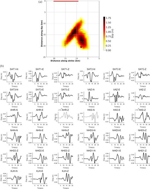
In order to obtain the spatial and temporal evolution of the slip for M1 and M2, we invert near-field strong motion displacement time-series recorded by 11 three-components SSA-2 Kinemetrics digital accelerometers from the ISMN. The stations are located at distances from 7 to 30 km from the ruptured area (red triangles on Fig. 2a). The acceleration data are integrated twice into displacement. Mean and trend of the waveforms are subtracted. Since all stations have their own orientation, we rotate their horizontal components to an NS/EW reference system.


(a) Source-station configuration that recorded the 2012 Ahar–Varzaghan earthquake doublet. Stars are the M1 and M2 epicentres. Triangles show strong motion stations positions of the ISMN. Solid lines are the surface rupture traces following the earthquake doublet. Squares show the nearby cities. (b) and (c) Observed displacements of M1 (b) and M2 (c) main shocks at the stations shown in (a), and bandpass filtered in the frequency range of 0.1–0.5 Hz. Name of each station and component is on top of the waveforms. The noisy components of M1 (AHR-Z and HAS-N) and M2 (HAS-N), plotted in thin lines are not used for the inversions.
The waveforms are cut using a time window of 25.6 s starting from the respective origin times. Then, the data are bandpass filtered using a Butterworth acausal filter for both M1 and M2, in the frequency band 0.1–0.5 Hz. We observed some low-frequency noises at some stations which limited us to use only frequencies higher than 0.1 Hz. Also the noisy components of M1 (AHR-Z and HAS-N) and M2 (HAS-N) are not used during the inversions (Figs 2b and c). The high cut-off frequency is chosen considering the resolution of the crustal velocity model of the area, which was retrieved from accurately located (<2 km error) aftershocks (Momeni & Tatar 2018, Table 2).
The crustal velocity model of the Ahar–Varzaghan area retrieved from 1-D inversion of the locally recorded aftershocks (Momeni & Tatar 2018).
| After Momeni & Tatar (2018) | |||||
|---|---|---|---|---|---|
| Depth of layer top (km) | Vp (km s−1) | Vs (km s−1) | Density (g cm−3) | Qp | Qs |
| 0.0 | 4.58 | 2.44 | 2.5 | 400 | 200 |
| 2.0 | 5.65 | 3.11 | 2.6 | 600 | 300 |
| 4.0 | 5.92 | 3.34 | 2.7 | 700 | 350 |
| 6.0 | 6.20 | 3.53 | 2.8 | 800 | 400 |
| 10.0 | 6.35 | 3.63 | 2.8 | 840 | 420 |
| 14.0 | 6.52 | 3.71 | 2.8 | 900 | 450 |
| 46.0 | 8.10 | 4.63 | 3.3 | 1500 | 750 |
3.2 Inversion strategy
In this study, we invert for the rupture process using the elliptical subfault approximation method. This method has been proposed by Vallee & Bouchon (2004) and has been successfully used to invert strong motion data by DiCarli et al. (2010), Ruiz & Madariaga (2011), Twardzik et al. (2012) and Ruiz & Madariaga (2013). This method approximates that the rupture occurs within a few elliptical patches (from 1 to usually 3) on a planar fault. This has the advantage to reduce the number of parameters to invert in comparison to the more commonly used rectangular subfaults parametrization.
Each elliptical patch is described by only nine parameters (five to describe its geometry and four to describe the source process within the elliptical patch, i.e. slip amplitude, slip duration, slip direction and onset time, see Fig. 3 for more details). While this method is not suited to retrieve fine details of the rupture process, it has the advantage to focus on the more robust features of the source process.
![Description of the elliptical subfault patches (based on Vallee & Bouchon 2004). Each patch can be described by the following parameters: (x0, y0): the two coordinates of the ellipse centre. (xa, xb): size of semimajor and semiminor axes, respectively. α: angle between the semimajor axis and the horizontal. smax: maximum slip. The slip distribution (S) inside each ellipse is defined as: S(x, y) = smax exp [− ($\frac{{{x^2}}}{{x_a^2}}$ + $\frac{{{y^2}}}{{x_b^2}}$)]. vr: the rupture velocity within each ellipse (after Twardzik et al. 2012).](https://oup.silverchair-cdn.com/oup/backfile/Content_public/Journal/gji/217/3/10.1093_gji_ggz100/3/m_ggz100fig3.jpeg?Expires=1750077829&Signature=4JhEOPEhYpJBn1jIkr4JYgSm1YY5QfblVFhE1CC3WMxU0Psle48LZuXSS7xqH7wJhLMRCfmOknFdXKuI6-8mtFHtW0ELljLXAs6JNDNjgDsupFdvS2QiegUuf87ka7d4PyMoh5~~a4t5hkFOs0jc0OLzv-KXDJeHVZXvIQxsxvwZf0CEVHFLxNop44lY664Q3obXisEs8PLGO4Brqh5n4B2Q4r13NnRq9Ds-BTqZpxnvpQqO-WbAJ9j-0~kOklCj6DgKCWD9YhpdtMrq7LRROrCrEXOWrSPRWyuwY5FmRDn1Z97j1MKXlaL2LcxSop71Sv1BybZecb5F-EU3-FjE7Q__&Key-Pair-Id=APKAIE5G5CRDK6RD3PGA)
Description of the elliptical subfault patches (based on Vallee & Bouchon 2004). Each patch can be described by the following parameters: (x0, y0): the two coordinates of the ellipse centre. (xa, xb): size of semimajor and semiminor axes, respectively. α: angle between the semimajor axis and the horizontal. smax: maximum slip. The slip distribution (S) inside each ellipse is defined as: S(x, y) = smax exp [− (|$\frac{{{x^2}}}{{x_a^2}}$| + |$\frac{{{y^2}}}{{x_b^2}}$|)]. vr: the rupture velocity within each ellipse (after Twardzik et al. 2012).
For both main shocks, we investigate the use of one, two and three elliptical patch(s) to describe the rupture process. First, we estimate the rupture of each main shock using one elliptical slip patch. Then we include more slip patches into the inversion. If the added ellipse did not improve the fit to the waveforms significantly and its parameters are unstable during the inversion, we favour the model with less elliptical patches.
Different inversions are carried out using the Neighborhood Algorithm (Sambridge 1999a, b). The algorithm searches for the optimal values of the source parameters by exploring a parameter space within pre-defined ranges for each parameter. For each inversion, we define ranges for slip (0.1–10 m), rupture speed (2–4 km s−1), rake (90–180°), rise time (0.1–10 s), length of the semi-axis (major = 1–20 km and minor = 1–20 km), the location of the centre of the ellipse (along strike = 1–35 km and along dip = 1–20 km), and the orientation with respect to the surface (0°–360°). The ranges for the different inversions are shown in Figs S1–S32 of the Supporting Information.
The exploration is carried out over a given number of iterations (up to 7000). During each iteration, 35 different rupture models are sampled by the Neighborhood Algorithm within the mentioned ranges. Then, the synthetics are computed for these models. In the next iteration, the algorithm samples 35 new rupture models. The new models are sampled by constructing bounded Voronoi cells around the 15 best-fitting models from the previous iteration (Appendices A and B, Supporting Information). At the end, the final rupture model is the one that fits best the data.
The Green's functions are computed using the AXITRA code (Cotton & Coutant 1997), which is based on discrete wavenumber method (Bouchon 2003), and we use the crustal model proposed by Momeni & Tatar (2018, Table 2). The similarity between the observed and calculated waveforms is measured using the cost function of Spudich & Miller (1990) in which the minimum obtained value of the function refers to the best similarity between data and synthetics.
We use the main shocks hypocentres relocated by Momeni & Tatar (2018). For each inversion, the hypocentre is allowed to move ± 1 km on the fault plane along strike and dip to allow small corrections for errors on the origin time. All the computations were carried out on the computer cluster of the High Performance facility of the International Centre for Theoretical Physics (ICTP).
First, because of the discrepancies in the results presented in Section 2, we decided to investigate different geometries for the two main shocks. Thus, for each earthquake, we perform kinematic finite-fault inversion assuming different geometries for the rupture plane. For each of the tested geometries, we use the same mentioned ranges for the source parameters.
Since there is a trade-off between the inverted parameters, instead of presenting only one particular final model, we present a family of models that fit equally well the data (i.e. Das & Kostrov 1990; Das & Kostrov 1994).
Once we obtained the best geometry for the fault plane, several additional inversions were performed in which we change the ranges of the parameters that are explored by the Neighborhood Algorithm (see Figs S1–S32, Supporting Information). This is to investigate other possible source models that satisfy the data. Indeed, if we do not change the assumed ranges, the Neighborhood Algorithm will sample the same rupture models for a given inversion. It also allows us to investigate if the final models depend much or not on the pre-defined parameters ranges.
For each main shock of the doublet, among all the inversions that we have run with different setups (∼50 inversions), we only show eight rupture models when one ellipse is used, and eight rupture models when two elliptical patches are used. To highlight the uncertainties associated with finite-fault inversion, the models that exhibit the most differences are chosen. Then, we use information about the observed surface rupture, the spatial distribution of aftershocks and the scalar seismic moment obtained from moment tensor inversion results, to choose a preferred model for each main shock. This is so that we can investigate the possible stress transfer from M1 to M2 and from both earthquakes on the NTF.
3.3 Rupture process of M1 (Mw6.5 earthquake)
3.3.1 The optimum geometry of M1
We examine different geometries for M1 using one and two elliptical patches. The aim is to find the optimum geometry based on the fit to the waveform and possibly its consistency with the observed surface rupture (Fig. A2 in Appendix A). We used the hypocentre relocated by Momeni & Tatar (2018), which is located at 46.84°E, 38.395°N, and at a depth of ∼8.5 km, and 10 km from the ground surface because of the local topography that reaches 1.5 km above sea level in this area (Fig. 2a).
Our preferred geometry is a fault plane with strike/dip = 88°/80° (see Appendix A). This geometry is close to the E-W nodal plane of the GCMT moment tensor (strike/dip/rake = 84°/84°/170°). Also, it is rather close to that of Momeni & Tatar (2018) (strike/dip = 268°/86°) obtained by moment tensor inversion using regional waveforms. However, it is different from that of Donner et al. (2015) who have obtained a dip of 45° for M1. Although Donner et al. (2015) argued that the dip angle was not well constrained in their inversion and could be steeper, they have excluded a vertical fault for M1. This may be due to the potential bias in aftershocks locations toward the north–northeast as it was highlighted by Momeni & Tatar (2018), and based on data of a local dense seismic network (for more information, see Fig. A3).
3.3.2 Rupture process of M1 using one elliptical slip patch
Fig. 4 shows the final rupture models of M1 resulting from the different inversions of the near-field displacement waveforms. Here, we used the best geometry determined in the previous subsection (i.e. strike/dip of 88°/80°S). The first eight rupture models in Fig. 4 describe M1 using one elliptical slip patch. These are the candidate models among the 50 independent inversion results, and that shows the most different features. This is to show the most variability for the candidate solutions.
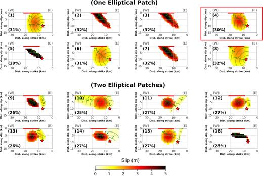
16 kinematic rupture models of M1 calculated by inverting near-field strong motion displacement time histories on the fault plane with strike/dip of 88°/80°S using one and two elliptical slip patches. Each subfigure is labelled with a number on the left top. The fault dimension is in kilometres. The X-axis show distance along strike and Y-axis is along downdip. The misfit of each model is written on the left bottom of each subfigure. The star is the earthquake hypocentre. Curved lines are positions of rupture front in time (seconds) after the origin time. Solid straight lines are positions of the reported surface rupture. The slip is saturated at 5 m. The best model (4) is highlighted by the box.
The convergence of inversion parameters is shown in Figs S1–S8 in the Supporting Information. We named the models with numbers from 1 to 8. All these models fit the data almost the same with a minimum wave misfit of ∼30 per cent. Each model is obtained using different setups for the inversions, i.e. using different ranges for the parameters that are sampled by the Neighborhood Algorithm (see Figs S1–S8 of Supporting Information). For all of these models the rupture direction, its duration and the rake value are well resolved. The slip extends to the west of hypocentre with large values located at shallow depths from 6 to 4 km, which is consistent with the calculated centroid of M1 (Donner et al. 2015; Momeni & Tatar 2018).
All models have almost the same source duration (between 5.1 and 5.6 s). The rake value is between 169° and 176° showing an almost pure right-lateral strike-slip mechanism. Except for Model 5, all rupture models reach the surface (Table A1 and Figs S1–S8, Supporting Information). This is consistent with the reported right-lateral offset at the surface by Copley et al. (2013) and Ghods et al. (2015, solid lines in Fig. 4).
However, we note that without imposing any constraints to the inversion, the final model parameters trade-off with each other (i.e. maximum slip, rupture dimension, rupture velocity and rise time). Among the models in which the slip reached to the surface the maximum slip changes from 2.2 to 6.3 m depending on the ellipse dimension. Considering the relatively stable rupture duration (5.1–5.6 s), the rupture velocity also changes from 2.2 to 3.0 km s−1, depending on the rupture dimension: models with faster rupture speed have longer rupture length (along both strike and dip) and smaller maximum slip (i.e. Model 8 compared to Model 6, Table A1).
In addition, the seismic moment and rise time cover relatively wide ranges. The released seismic moment ranges from 8.3E + 18 to 9.6E + 18 N·m, which is equal to or larger than the estimated scalar moment by regional waveform inversion (8.3E + 18 N·m, Momeni & Tatar 2018). The rise times also change between 1.1 and 2 s. We note that models with higher rise times exhibit higher rupture speeds, which is consistent with the results on dynamic simulations from Schmedes et al. (2010).
We used the ∼1 m right-lateral dislocation observed at the surface (Copley et al. 2013; Ghods et al. 2015), the distribution of aftershocks and the scalar seismic moment obtained from moment tensor inversion (Momeni & Tatar 2018) as constraints to choose the preferred model. The right-lateral dislocation of ∼1 m at the surface (solid lines in Fig. 4) does not match Models 2, 3, 5 and 7. Models 1, 6 and 8 have scalar moments >9.0 E + 18 N·m which is higher than the moment tensor inversion result (∼8.3 E + 18 N·m; Momeni & Tatar 2018). Thus, Model 4 is the model that best satisfies the external constraints.
3.3.3 Rupture process of M1 using two elliptical slip patches
When we invert the displacement time-series of M1 using two elliptical slip patches, the misfit of the kinematic rupture models reduces to lower values between 25–27 per cent (models named with numbers 9–16 in Figs 4 and A2b), which is expected since we are using more parameters. These models are also selected among 50 independent inversions in order to exhibit candidate solutions with the most discrepancies. The convergence of inversion parameters is shown in Figs S9–S16 in the Supporting Information. Similar to the rupture models with one slip patch, the rupture models with two slip patches show that the main moment release (∼86 per cent) is located west of the hypocentre and at shallow depths.
Meanwhile, the second slip patch contributes on average to only 14 per cent of the released seismic moment (Table A1). Fig. 4 shows that the second slip patch is unstable on the fault. Still, we note that in most of the models, this patch is located to the east of the hypocentre and the main slip patch. Overall, the two ellipse rupture models release less seismic moment (<8.0E + 18 N·m, Table A1) than the single-ellipse models. Also, the rake of the second slip patch is unstable and changes from pure reverse (Models 9, 10, 13 and 16) to right-lateral strike-slip (Models 11, 12, 14 and 15).
We also note that adding one patch to the inversion only slightly improve the waveform fit of the first arriving phases of the E-W components of stations SAT1, SAT3, NHD1, NHD2 and NHD3 (for example see the waves in the rectangles shown in Figs S4 and S12, Supporting Information). From these conclusions, we believe that our data cannot reliably constraint the source parameters of the second slip patch (for more information see the convergence of the model parameters in Figs S9–S16, Supporting Information).
3.4 Rupture process of M2 (Mw6.3 earthquake)
3.4.1 The optimum geometry of M2
As for M1, we first explore different trial geometries for M2 using one and two elliptical patches. Here, our goal is to find the geometry that provides the best fit to the waveforms and that is consistent with the moment tensor inversion results (for more information see Figs B1 and B2 in Appendix B). We use the hypocentre from Momeni & Tatar (2018), and that is located at 46.79°E, 38.44°N and at a depth of ∼16.5 km (18 km from the ground surface since the local topography is 1.5 km above sea level in this area) (Fig. 2a).
Our preferred geometry for the fault plane is strike/dip = 256°/60°. It provides the best waveforms fit, the same seismic moment and centroid depth than that obtained by Momeni & Tatar (2018) (3.2E + 18 N·m and 11 km ,respectively, for more information see Appendix B).
We also inverted the data for M2 source parameters on the geometries proposed or used by Alipour (2013), Donner et al. (2015), Zafarani et al. (2015), Yadav et al. (2016) and Yazdi et al. (2018). We did not obtain a good fit to the waveforms for these geometries. The reason of such inconsistency is probably because of the errors in the location of the two main shocks and aftershocks that are used to investigate the geometry of the causative faults in previous studies, as highlighted by Momeni & Tatar (2018). Indeed, no lineament of aftershocks is observed by Momeni & Tatar (2018) in the N-S direction, opposite to what has been proposed in some studies (Donner et al. 2015; Yadav et al. 2016; Yazdi et al. 2018). Instead, the obtained geometry for M2 is consistent with that obtained by Ghods et al. (2015) and Momeni & Tatar (2018).
3.4.2 Rupture process of M2 using one elliptical slip patch
Fig. 5 shows the final rupture models of M2 resulting from the inversion of the near-field displacement waveforms. Here, the rupture models are calculated using a planar fault with a strike/dip of 256°/60°N and that is consistent with the results from the previous subsection. The first eight rupture models in Fig. 5 (named with numbers from 1 to 8) are describing M2 using a single elliptical slip patch. As previously, we show candidate solutions with the most differences among 50 inversions in order to highlight the variability of the solution. The convergence of inversion parameters is shown in Figs S17–S24 in the Supporting Information. They reach a misfit of ∼36–39 per cent.
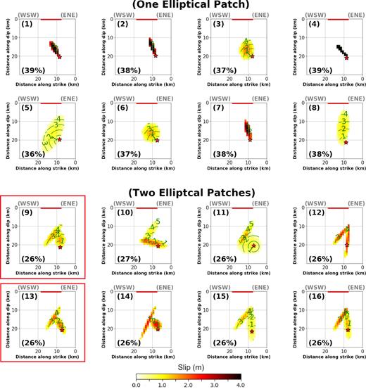
16 kinematic rupture models of M2 calculated by inverting near-field strong motion displacement time histories on the fault plane with strike/dip of 256°/60°S using one and two elliptical slip patches. Each subfigure is labelled with a number on the left top. The fault dimension is in kilometres. The X-axis show distance along the strike (256°) and Y-axis is along downdip. The misfit of each model is written on the left bottom of each subfigure. The star shows the earthquake hypocentre. Curved lines are positions of rupture front in time (seconds) after the origin time. Solid lines are positions of the reported surface rupture. The slip is saturated at 4 m. The best models (9 and 13) are highlighted by the boxes.
Among all these rupture models, some similarities are observed on the rupture direction and the rake value. For all of them, the rupture propagates towards shallower depths and to the west, and none of them reach the surface. The rake is well resolved. Indeed, all models have rakes of 130°–140°, exhibiting oblique reverse mechanisms (see Table B2, and Figs S17–S24, Supporting Information). All of them show that the area of maximum slip is located at depths from 14 to 10 km, consistent with the centroid depth from moment tensor inversions by previous studies (e.g. Donner et al. 2015; Momeni & Tatar 2018). However, some parameters like the maximum slip, rupture speed, rupture duration and scalar seismic moment are rather uncertain (Table B2). The scalar seismic moment ranges between 2.8E + 18 N·m to 3.5E + 18, close to the scalar moment estimated by Momeni & Tatar (2018) (∼3.2E + 18 N·m). Meanwhile, the rupture speed shows significant uncertainty, from subshear (2.3 km s−1) to supershear (3.9 km s−1, the average shear wave velocity in the ruptured area being 3.7 km s−1). This explains why the rupture duration ranges between 3.3 and 4.4 s. These uncertainties can be either due to the simplicity of the rupture model or due to the data quality.
3.4.3 Rupture process of M2 using two elliptical slip patches
To test for more complex rupture model, we invert the displacement time-series using two elliptical slip patches. The misfit of the kinematic rupture models is reduced (26–27 per cent) by about 13 per cent compared to models with one elliptical patch (named with numbers from 9 to 16 in Fig. 5, and Figs B2 and B3). In particular, the fit of SAT1, SAT2 and SAT3, which are located near M2 show great improvement. Thus, the visible improvement of the fit to the waveforms when using two slip patches compared to one slip patch supports the existence of a second slip patch during the rupture of M2 (see Table B2, and Figs S25–S32, Supporting Information).
The stability of the two slip-patches rupture models for M2 is investigated by looking in details on the eight final rupture models of the M2 (Models from 9 to 16, Fig. 5). As usual, we highlight the variability of the candidate solution by choosing the most different rupture models from 50 different inversions. The convergence of inversion parameters is shown in Figs S25–S32 in the Supporting Information.
The final models show some similar features. The slip propagates mostly toward shallower depths and to the west and is confined at depths below 8 km. This is again consistent with the calculated centroid depth for M2 at ∼11 km (e.g. Donner et al. 2015; Momeni & Tatar 2018). The rakes are resolved well for both rupture patches: the first patch (the deeper patch located on the east) exhibits an almost pure right-lateral strike-slip mechanism (rake 172°–180°), while the second patch (the shallow ellipse on the west) has a reverse mechanism (rake 104°–115°) (Table B2, and Figs S25–S32, Supporting Information). The total rupture time of M2 is almost the same for all the models and change from 4.5 to 5.2 s.
The estimated seismic moment released varies between ∼3.24E + 18 and 3.89E + 18 N·m which is almost equal to or larger than the estimated scalar moment from Momeni & Tatar (2018) (∼3.2E + 18 N·m). Both slip patches contribute almost to the same amount of seismic moment release (Table B2). Thus, it seems that M2 is more complex, since is best described by two patches with two different mechanisms and comparable scalar seismic moments.
Once again we observe that without any constraints on the inversion, the parameters of the final models trade-off with each other. The rupture speed of the first (eastern) patch is very uncertain and can change from subshear (2.7 km s−1) to supershear (4.0 km s−1) (the average shear wave velocity in the ruptured area being 3.7 km s−1). The second (western) slip patch has a better resolution on the rupture speed. It shows a lower rupture speed ranging from 2.2 to 2.8 km s−1. However, the results are showing a consistency that the first patch with a strike-slip mechanism is more probable to rupture with a higher speed.
We used the aftershocks distribution and the obtained scalar seismic moment of this event from moment tensor inversion to choose the preferred M2 rupture model. The only models that have almost the same scalar seismic moment to the moment tensor inversion (<3 per cent different) are Models 9, 13 and 15. Other models have a scalar seismic moment that is higher than 3.4 E + 18 N·m and up to 3.9 E + 18 N·m. Among Models 9, 13 and 15, we find that Model 15 has slip at depths deeper than 16 km. However, all of the precisely located aftershocks (<2 km error) were reported at depths shallower than ∼15 km (Momeni & Tatar 2018), i.e. 1.5 km above the hypocentre of M2. Thus, the likelihood that some slip occurred deeper than 16 km is low.
The remaining models (9 and 13) satisfy both criteria: (1) they match the distribution of aftershocks and (2) their centroid and scalar moment are almost the same as the moment tensor inversion results. Both of them show almost the same distribution of slip and the same rakes of ∼177 and ∼113 for the first and second slip patches, respectively. The main difference is in the rupture speed of the first slip patch (2.8 and 3.75 km s−1 for Models 13 and 9, respectively).
One reason for such unstable rupture velocity is the uncertainty on the location of the slip patches with respect to the location of the hypocentre. Indeed, the distance from the hypocentre to the second slip patch is ∼10 km in Model 9 compared to ∼7 km in Model 13. Consequently, the rupture needs to be faster in Model 9 in order to not overestimate the well-resolved rupture duration. Thus, we believe that the unstable rupture speed for the hypocentral patch is a hint that it cannot be resolved well by our data.
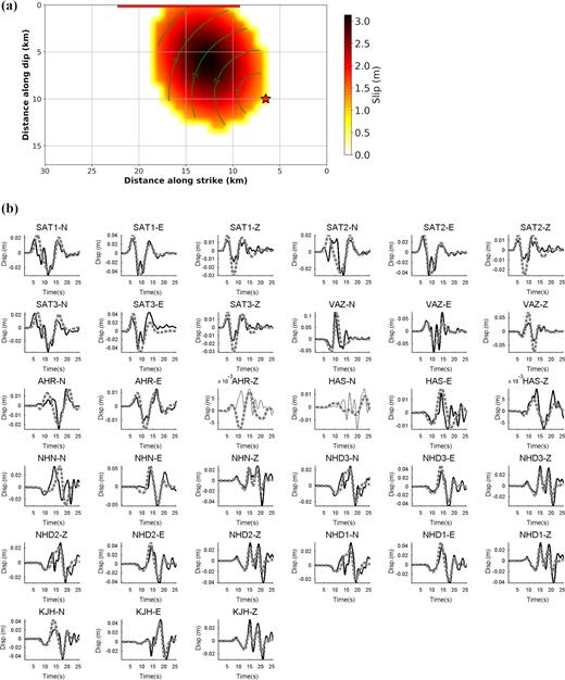
As supershear is only reported for very few cases, mostly on very long planar fault (e.g. Robinson et al. 2010), we note that a rupture of 3.75 km s−1 is rather high for an Mw = 6.3 event. However, Models 9 and 13 fit the data equally well, and we cannot argue for sure that 3.75 km s−1 is not possible for the hypocentral patch. This is why we have decided to average the two models (see Fig. 7a), and to use it as our preferred rupture model since it shows a reliable misfit of 27 per cent (Fig. 7b).
4 PREFERRED RUPTURE MODELS FOR M1 AND M2
We have evaluated different geometries and rupture models for M1 and M2, considering one and two elliptical slip patches (Section 3). Wide ranges of model parameters have been examined in order to explore a large variability of models that can fit the near-field strong motions.
Our preferred rupture model for M1 (Model 4) has one slip patch with semimajor and semiminor axes of 7.4 and 5.9 km, respectively (Fig. 6a). This model shows that the nucleation of M1 took place at a depth of ∼8.5 km (10 km from the ground surface) about 4 km east of the eastern termination of the surface rupture. The slip mostly extends toward the shallow depths and to the west of the hypocentre with an average speed of 2.4 km s−1. The maximum slip is ∼3.1 m and occurs from 6 to 4 km depths. The rupture lasts for ∼5.6 s, similar to the source time function obtained by SCARDEC (http://scardec.projects.sismo.ipgp.fr/#; last accessed 2016 May). It reaches the surface and matches with ∼8 km of the 12 km of observed surface rupture. It releases a scalar seismic moment of 8.41E + 18 N·m, almost the same as that estimated from moment tensor inversion (Momeni & Tatar 2018).
(a) Preferred rupture model for M1. Notations are the same as Fig. 4. (b) The waveform fit for the preferred model for M1. Black solid lines and grey dashed lines are observed and calculated displacements, respectively. AHR-Z and HAS-N components are not used during the inversion. Instead, we only compute them by forward modelling. Other notations are the same as Fig. 2(b).
(a) Preferred rupture model for M2 resulted from an average of the Models 9 and 13 (shown in Fig. 5). Notations are the same to Fig. 5. (b) The waveform fit for the preferred model for M2. Black solid lines and grey dashed lines are observed and calculated displacements, respectively. HAS-N component is not used during the inversion, and is only computed by forward modelling. Other notations are the same as Fig. 2(c).
For M2, we observe two slip patches with different mechanisms and comparable magnitudes. The final model shows that M2 nucleated at a depth of ∼16.5 km and the rupture propagates mostly toward shallow depths, and is composed of two major slip patches. The rupture of the first patch lasts for 2.6 s and that has a rather high speed (>2.8 km s−1), and an almost pure strike-slip mechanism. Meanwhile, the western patch is shallower, and ruptures at a slower speed (∼2.5 km s−1). It also shows a reverse mechanism. The rupture duration of the second patch is ∼2.5 s. Both patches release a total seismic energy of ∼3.27E + 18 N·m in 5.1 s.
5 CORRELATION BETWEEN SLIP MODELS OF THE DOUBLET AND DISTRIBUTION OF AFTERSHOCKS
Fig. 8(a) shows the hypocentres of 2516 accurately located aftershocks (location error <2 km and azimuthal gap <170°) that have occurred within the first 24 d after the main shocks, together with 50 focal mechanisms for the aftershocks with magnitude greater than 3, and calculated based on polarity of the first P-wave arrivals (Momeni & Tatar 2018). The network consists of 17 stations that were installed 2 d after the main shocks and operated for 22 d. Fig. 8(b) shows the east–west vertical cross-section (AA’) parallel to the surface rupture. We also show on the cross-section the slip distributions of M1 and M2 together with the aftershocks hypocentres.
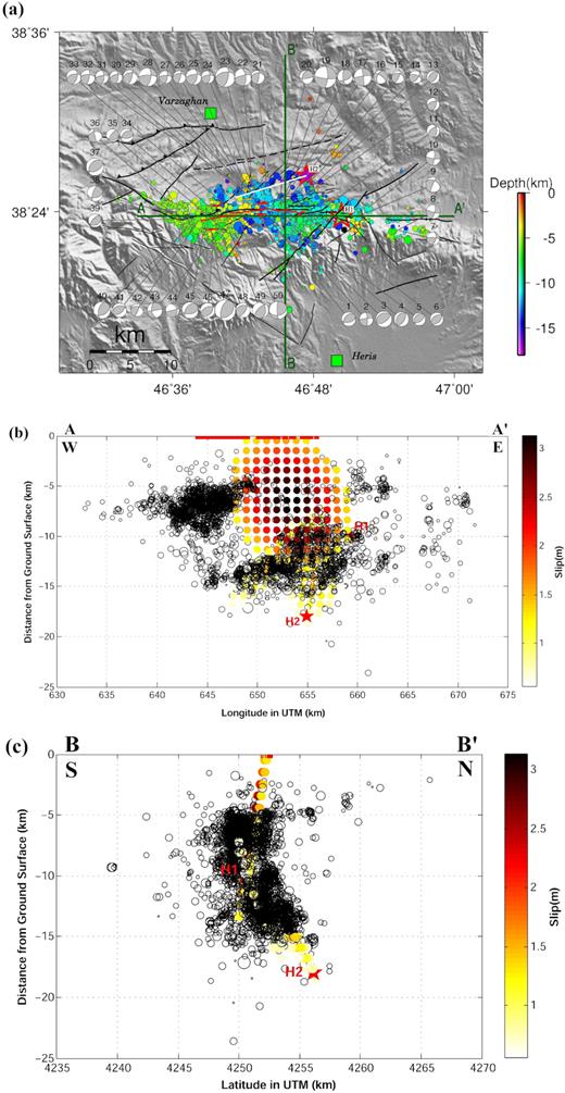
(a) Locations and focal mechanisms of the earthquake doublet and 2516 precisely located aftershocks within the first 24 d (after Momeni & Tatar 2018). Stars and circles are the two main shocks and aftershocks epicentres, respectively. H1 and H2 are the hypocentres of M1 and M2, respectively. Colours exhibit the hypocentral depth of each event. The white line represents the position of the M2 causative fault plane at its nucleation depth at 16.5 km. Solid lines are the surface rupture traces. Black lines are active faults of the area (Ghods et al. 2015). Focal mechanisms of the 50 M ≥ 3 aftershocks are shown in grey. Their hypocentre error is <1.5 km and their nodal plane errors are <10° (after Momeni & Tatar 2018). Black lines are the active faults. Squares show the nearby cities. Solid lines with signs of AA′ and BB′ represent the positions of vertical cross-sections shown in (b) and (c). (b) and (c) Open circles are aftershocks (0.5 < M < 5.2) and coloured circles show the slip distribution of M1 and M2, with colours representing the slip amplitude. Stars are the hypocentres of M1 and M2 and are labelled by H1 and H2, respectively. Solid lines are the surface ruptures. Coordinates are in UTM (km). (b) East to west cross-section AA′ shows the main gap of aftershocks activity that separates them in two distinct clusters. The maximum slip which corresponds to the main slip patch of M1 is located within this gap. Some aftershocks are observed toward the far east of the slip models of the doublet. (c) South to north cross-section BB′ showing the distribution of aftershocks. We observe the aftershocks closely follow the dip of the fault planes of the two main shocks.
Aftershocks are distributed from the near surface (∼ 2 km depth) down to a depth of ∼15 km in the EW direction over 40 km length and 15 km wide. They surround the slipping regions of M1, while this pattern is not as clear for M2. We also note that the focal mechanisms of the aftershocks correlate well with that of the main shocks. Few focal mechanisms are similar to M1 (i.e. focal mechanisms numbered 7, 8 and 10), and the northern cluster of aftershocks shows mostly the same mechanisms as M2 (i.e. focal mechanisms numbered 21–33) (Fig. 8a). The aftershocks on the western cluster of seismicity are located in the rupture direction of M1 and M2 and are mostly showing reverse focal mechanisms, with the two nodal planes roughly striking NE-SW (i.e. focal mechanisms 34–50). These focal mechanisms are different from the ones of M1 and M2.
The slip model of M1 matches the surface ruptures (Figs 8b and c) and aftershocks align well along the fault planes of the two earthquakes. We note that M2 rupture joins the area of M1 rupture at a depth of ∼8 km and is possibly connected to it, or crosses it from underneath M1 toward the south.
A low aftershock activity is observable close to the hypocentre of M2 (Fig. 8c), and above it, the aftershocks mostly show pure strike-slip to reverse mechanism. This is probably due to a complex stress field caused by the occurrence of M1 and M2 in a close distance.
6 STRESS INTERACTION BETWEEN M1, M2 AND NTF
The stress tensor produced by the kinematic source model of M1 is calculated on a 3-D grid in the Ahar–Varzaghan area using the method by Wang et al. (2003). This is based on the dislocation theory in a multilayered model. We use the 1-D crustal velocity model of the area retrieved from precisely located aftershocks (Momeni & Tatar 2018, Table 2) and a Poisson ratio of ∼0.25 obtained from a Vp/Vs ratio of 1.74 (Momeni & Tatar 2018). The Coulomb stress field is calculated on an optimally oriented rupture of M2, and by considering both mechanisms of the two slip patches that we observe, i.e. strike-slip and reverse.
Fig. 9 shows the static Coulomb stress changes induced by M1 on M2 using a coefficient of friction of 0.7. The results show a positive static stress increase of up to over 10 bars on the fault plane of M2, and that coincides with the area where M2 has released most of its moment. We note that the high correlation between the stress changes caused by M1 and the slip distribution of M2 provides an additional clue that the inversions have indeed retrieve the robust features of both main shocks. This is also more remarkable since this match is not resulting from a constraint used during the inversion. Such high positive stress transfer is believed to be able to trigger an earthquake (e.g. Toda et al. 1998; Anderson & Johnson 1999; Stein 1999).
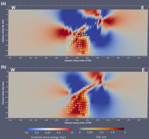
(a) and (b) Coulomb stress transfer induced by M1 on the optimally oriented fault plane of M2 (strike/dip = 256°/60°) considering (a) the pure strike-slip and (b) reverse mechanisms. This corresponds to the first (eastern) and second (western) slip patches of M2, respectively. The stress field is saturated to ± 10 bars. The slip during M2 is shown by coloured squares. Star shows M2 hypocentre (H2).
The nucleation of M2 took place in the strike-slip patch with about 3 bars of positive stress change. This patch is located inside a positive stress change that is up to 6 bars (Fig. 9a). The rupture area of the second (western) slip patch, the one with a reverse mechanism and that host the larger release of energy is nicely controlled by a positive Coulomb stress change of more than 10 bars (Fig. 9b).
Yazdi et al. (2018) propose that M1 do not transfer positive stress on the ∼E-W striking nodal plane of the M2 focal mechanism. However, we believe that the discrepancy in the results compared to ours is caused by the differences in the source models as well as the proposed location for the hypocentres of M1 and M2. Indeed, Yazdi et al. (2018) assume that both hypocentres are at a depth of 10 km, while we use 10 km for M1 and 15 km for M2.
Figs 9(a) and (b) show that the rupture of M2 stops when it reaches the region of high negative Coulomb stress change (∼ −10 bars) induced by M1. The slip distribution of M2 is in fact very well delimited by the negative Coulomb stress field induced by M1. Also, the mechanism of faulting for the two slip patches of M2 seems to be very well controlled by the stress field.
We also measure the amount of static Coulomb stress induced by both main shocks of the doublet on the optimally oriented NTF. Our calculation shows that the doublet has transferred a positive Coulomb stress on the eastern segment of NTF of ∼0.1 and ∼0.02 bars for M1 and M2 respectively (Fig. 10). As discussed earlier, this segment has not ruptured since 1721 during an M 7.6–7.7 earthquake, and it is brought closer to failure by this doublet. We also calculate negative Coulomb stresses of over −0.1 bars from the doublet on the central and western segments of the NTF (mostly within a radius of 30 km from the Tabriz city), which coincides partly with the ruptured area of the 1780 M7.4 historical event.
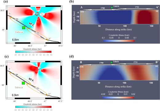
Coulomb stress field transferred from M1 on the optimally oriented fault of NTF in map view (a) for a depth of 6 km, and (b) a vertical AA’ section along the NTF. (c) and (d) are the same sections for M2 produced Coulomb stress field on the optimally oriented NTF. Stars show the main shocks epicentres. Solid lines near the main shocks are the surface ruptures. Ellipses represent the ruptured areas during the 1721 M7.6–7.7 and the 1780 M7.4 events. Square shows the Tabriz city. The black line is the North Tabriz Fault labelled as NTF. The stress fields are saturated at ± 0.5 bars. Black vectors on (b) and (d) show the rupture extent of the 1721 and 1780 historical earthquakes.
7 DISCUSSION AND CONCLUSION
We investigated the robust features of the rupture process and the fault geometries of the Ahar–Varzaghan earthquake doublet. This is done by inverting the near-field strong motion displacement time histories, using the elliptical subfault approximation method. Our inversion demonstrates that M1 and M2 have occurred on two different faults: M1 nucleates near ∼4 km east of the eastern termination of the surface rupture and at a depth of ∼8.5 km. The rupture evolves mostly toward the west and to the surface with speed of ∼2.4 km s−1 on an ∼EW striking fault plane (N088E) with a dip of ∼80° to the south. It exhibits a right-lateral strike-slip mechanism and releases a total seismic moment of 8.41E18 N·m. The maximum slip of ∼3.1 m obtained between 6 and 4 km depth. We also observe a slip of ∼1 m near the surface, which is consistent with the observed dislocation on the surface (Copley et al. 2013).
M2 occurs on an ENE-WSW oriented (∼N256°) fault plane with the dip of ∼60° toward the north. The rupture starts about 11 min after M1, and about 5 km west and 4 km north of the M1 hypocentre and at a depth of ∼16.5 km. The slip propagates upward and then laterally to the west, in two major slip patches with comparable maximum slip (∼1.6 m) and moment (∼1.6E18 N·m). The eastern patch is right above the hypocentre; rupture propagates relatively fast with speed of higher than 2.8 km s−1. It has an almost pure right-lateral strike-slip mechanism. The western (second) patch has a reverse mechanism (rake ∼112°) and ruptures with a speed of ∼2.5 km s−1. All models for M2 show that the slip is confined to depths ranging from about 16.5 to 8 km.
Thus, it appears that M1 is the cause of the observed 12 km surface rupture. Because we do not have reliable GPS position right after the earthquakes, we cannot assess how much is coseismic and afterslip. The source models of the earthquake doublet correlate reasonably well with the aftershock distribution as well as with the focal mechanisms of earthquakes with M > 3. In particular, aftershocks are not distributed where the largest slip patch (with a maximum slip of ∼3.1 m) of M1 is located, but surrounds it (Fig. 8). The observation of aftershocks surrounding high slipping regions seems to be a consistent feature of a large earthquake (see Henry & Das 2002).
All of the previous studies confirm that M1 plane has an ∼E-W strike and its rupture reached to the surface. However, they do not agree on the dip of the fault plane. Our inversions show a very steep dipping plane toward the south (80°S), relatively close to the obtained dip by Copley et al. (2013) (90°, fixed), GCMT result (84°S) and Momeni & Tatar (2018) (86°N), and close to the used vertical dip fault planes by Yazdi et al. (2018) and Amini et al. (2018). Instead, Donner et al. (2015) and Ghods et al. (2015) proposed a northward dip fault plane for M1. Among these studies, Amini et al. (2018) are the only one that used almost the same fault geometry to us in order to obtain the rupture model of M1. However, their slip model is distributed over a 40 × 20 km2 area which is extend longer and deeper than our model (11 × 12 km2). This is because they use IRSC located aftershocks as a constraint. We note that Momeni & Tatar (2018) did not observe aftershocks activity at depths deeper than 15 km. A maximum slip of ∼1.3 m is reported by Amini et al. (2018), and is located 10 km west of the hypocentre and at a depth of ∼4 km. The slip amplitude is lower than our obtained maximum slip (3.1 m), but the slip patches are located at the same position. They also reported a relatively faster rupture speed of ∼2.8 km s−1 for this event, compared to our result (2.4 km s−1).
The slip models obtained by Alipour (2013) and Yadav et al. (2016) show maximum slip of 1.5 m and 1.3 m, respectively, and located at very shallow depths (near the surface). In that case, the slip amplitude is also less than our obtained value (3.1 m), but this time, the slip patches are located at different positions than for our model. Finally, the proposed slip model by Yazdi et al. (2018) shows a relatively low maximum slip value of 0.8 m on a 19 × 14 km2 slip patch, on a fault that has the same strike than the observed surface rupture and a vertical dip. This is less than our obtained maximum slip (3.1 m) and that of Amini et al. (2018) (1.3 m).
Our obtained ENE-WSW striking fault plane for M2 is different from previous studies that have investigated the slip of this earthquake (e.g. Alipour 2013; Donner et al. 2015; Yadav et al. 2016; Amini et al. 2018; Yazdi et al. 2018). However, we are the first to analyse the rupture model for this earthquake. Thus, we cannot make a fair comparison between our obtained M2 rupture model and previous ones. Still, Ghods et al. (2015) and Rezapour (2016) have proposed geometries for M2 fault that are close to our obtained geometry, although these authors have not investigated the source parameters of the M2.
The 3-D static stress modelling of M1 on the optimally oriented fault of M2 shows a strong correlation between areas with high positive Coulomb stress values and the ruptured area of M2, for both the strike-slip and reverse mechanisms observed for the two slip patches of M2. The maximum slip area of M2 (∼1.6 m at depths ranging from 10 to 13 km) lies within high positive Coulomb stress area induced by M1 (up to 10 bars). This strongly suggests that M2 has been triggered by the static Coulomb stress changes induced by M1.
Towards shallow depths, the high negative Coulomb stress changes (up to −10 bars) seem to behave as a barrier and stop the continuation of the M2 rupture (Fig. 9). The striking match between the Coulomb stress transfer induced by M1 with the slip distribution of M2 gives us extra confidence regarding the obtained rupture model of both earthquakes.
The cumulative static Coulomb stress changes of M1 and M2 on the optimally oriented fault of NTF shows a positive load of >0.1 bars on its eastern segment (Fig. 10). Such a small increase in static stress is known to be enough to trigger earthquakes especially on potentially active faults (e.g. Stein 1999). It is important to note that the NTF has not experienced any devastating earthquake on its eastern segment since the 1721 M7.6–7.7 event. Thus, the occurrence of this doublet may have increased the seismic hazard on Tabriz city that is currently hosting over 2 million people.
SUPPORTING INFORMATION
Figure S1. (A) The wave fit of the M1 final Model 1 (Table A1). (B) The defined ranges for the model parameters and the convergence of each parameter of the M1 final Model 1. The range of the misfit function during inversion is shown in (g).
Figure S2. (A) The wave fit of the M1 final Model 2 (Table A1). (B) The defined ranges for the model parameters and the convergence of each parameter of the M1 final Model 2. The range of the misfit function during inversion is shown in (g).
Figure S3. (A) The wave fit of the M1 final Model 3 (Table A1). (B) The defined ranges for the model parameters and the convergence of each parameter of the M1 final Model 3. The range of the misfit function during inversion is shown in (g).
Figure S4. (A) The wave fit of the M1 final Model 4 (Table A1). (B) The defined ranges for the model parameters and the convergence of each parameter of the M1 final Model 4. The range of the misfit function during inversion is shown in (g).
Figure S5. (A) The wave fit of the M1 final Model 5 (Table A1). (B) The defined ranges for the model parameters and the convergence of each parameter of the M1 final Model 5. The range of the misfit function during inversion is shown in (g).
Figure S6. (A) The wave fit of the M1 final Model 6 (Table A1). (B) The defined ranges for the model parameters and the convergence of each parameter of the M1 final Model 6. The range of the misfit function during inversion is shown in (g).
Figure S7. (A) The wave fit of the M1 final Model 7 (Table A1). (B) The defined ranges for the model parameters and the convergence of each parameter of the M1 final Model 7. The range of the misfit function during inversion is shown in (g).
Figure S8. (A) The wave fit of the M1 final Model 8 (Table A1). (B) The defined ranges for the model parameters and the convergence of each parameter of the M1 final Model 8. The range of the misfit function during inversion is shown in (g).
Figure S9. (A) The wave fit of the M1 final Model 9 (Table A1). (B) The defined ranges for the model parameters and the convergence of each parameter of the M1 final Model 9. The range of the misfit function during inversion is shown in (m).
Figure S10. (A) The wave fit of the M1 final Model 10 (Table A1). (B) The defined ranges for the model parameters and the convergence of each parameter of the M1 final Model 10. The range of the misfit function during inversion is shown in (m).
Figure S11. (A) The wave fit of the M1 final Model 11 (Table A1). (B) The defined ranges for the model parameters and the convergence of each parameter of the M1 final Model 11. The range of the misfit function during inversion is shown in (m).
Figure S12. (A) The wave fit of the M1 final Model 12 (Table A1). (B) The defined ranges for the model parameters and the convergence of each parameter of the M1 final Model 12. The range of the misfit function during inversion is shown in (m).
Figure S13. (A) The wave fit of the M1 final Model 13 (Table A1). (B) The defined ranges for the model parameters and the convergence of each parameter of the M1 final Model 13. The range of the misfit function during inversion is shown in (m).
Figure S14. (A) The wave fit of the M1 final Model 14 (Table A1). (B) The defined ranges for the model parameters and the convergence of each parameter of the M1 final Model 14. The range of the misfit function during inversion is shown in (m).
Figure S15. (A) The wave fit of the M1 final Model 15 (Table A1). (B) The defined ranges for the model parameters and the convergence of each parameter of the M1 final Model 15. The range of the misfit function during inversion is shown in (m).
Figure S16. (A) The wave fit of the M1 final Model 16 (Table A1). (B) The defined ranges for the model parameters and the convergence of each parameter of the M1 final Model 16. The range of the misfit function during inversion is shown in (m).
Figure S17. (A) The wave fit of the M2 final Model 1 (Table B2). (B) The defined ranges for the model parameters and the convergence of each parameter of the M2 final Model 1. The range of the misfit function during inversion is shown in (g).
Figure S18. (A) The wave fit of the M2 final Model 2 (Table B2). (B) The defined ranges for the model parameters and the convergence of each parameter of the M2 final Model 2. The range of the misfit function during inversion is shown in (g).
Figure S19. (A) The wave fit of the M2 final Model 3 (Table B2). (B) The defined ranges for the model parameters and the convergence of each parameter of the M2 final Model 3. The range of the misfit function during inversion is shown in (g).
Figure S20. (A) The wave fit of the M2 final Model 4 (Table B2). (B) The defined ranges for the model parameters and the convergence of each parameter of the M2 final Model 4. The range of the misfit function during inversion is shown in (g).
Figure S21. (A) The wave fit of the M2 final Model 5 (Table B2). (B) The defined ranges for the model parameters and the convergence of each parameter of the M2 final Model 5. The range of the misfit function during inversion is shown in (g).
Figure S22. (A) The wave fit of the M2 final Model 6 (Table B2). (B) The defined ranges for the model parameters and the convergence of each parameter of the M2 final Model 6. The range of the misfit function during inversion is shown in (g).
Figure S23. (A) The wave fit of the M2 final Model 7 (Table B2). (B) The defined ranges for the model parameters and the convergence of each parameter of the M2 final Model 7. The range of the misfit function during inversion is shown in (g).
Figure S24. (A) The wave fit of the M2 final Model 8 (Table B2). (B) The defined ranges for the model parameters and the convergence of each parameter of the M2 final Model 8. The range of the misfit function during inversion is shown in (g).
Figure S25. (A) The wave fit of the M2 final Model 9 (Table B2). (B) The defined ranges for the model parameters and the convergence of each parameter of the M2 final Model 9. The range of the misfit function during inversion is shown in (m).
Figure S26. (A) The wave fit of the M2 final Model 10 (Table B2). (B) The defined ranges for the model parameters and the convergence of each parameter of the M2 final Model 10. The range of the misfit function during inversion is shown in (m).
Figure S27. (A) The wave fit of the M2 final Model 11 (Table B2). (B) The defined ranges for the model parameters and the convergence of each parameter of the M2 final Model 11. The range of the misfit function during inversion is shown in (m).
Figure S28. (A) The wave fit of the M2 final Model 12 (Table B2). (B) The defined ranges for the model parameters and the convergence of each parameter of the M2 final Model 12. The range of the misfit function during inversion is shown in (m).
Figure S29. (A) The wave fit of the M2 final Model 13 (Table B2). (B) The defined ranges for the model parameters and the convergence of each parameter of the M2 final Model 13. The range of the misfit function during inversion is shown in (m).
Figure S30. (A) The wave fit of the M2 final Model 14 (Table B2). (B) The defined ranges for the model parameters and the convergence of each parameter of the M2 final Model 14. The range of the misfit function during inversion is shown in (m).
Figure S31. (A) The wave fit of the M2 final Model 15 (Table B2). (B) The defined ranges for the model parameters and the convergence of each parameter of the M2 final Model 15. The range of the misfit function during inversion is shown in (m).
Figure S32. (A) The wave fit of the M2 final Model 16 (Table B2). (B) The defined ranges for the model parameters and the convergence of each parameter of the M2 final Model 16. The range of the misfit function during inversion is shown in (m).
Please note: Oxford University Press is not responsible for the content or functionality of any supporting materials supplied by the authors. Any queries (other than missing material) should be directed to the corresponding author for the paper.
ACKNOWLEDGEMENTS
SM acknowledges support from the ICTP-Regione Friuli-Venezia Giulia programme. This study was supported by International Institute of Earthquake Engineering and Seismology (IIEES), under the project number 5371–597. CT was funded by Centre National d'Etdues Spatiales and by the ANR JCJC E-POST. We are grateful to the Building and Housing Research Center (BHRC) for providing the strong motion data. We greatly thank Prof Eiichi Fukuyama and two anonymous reviewers for comments and suggestions that improved the manuscript. Most of the calculations were done using processors of the ARGO cluster belong to the High Performance Computing (HPC) center of the ICTP, Trieste, Italy. Figures are plotted using Generic Mapping Tools (GMT, http://gmt.soest.hawaii.edu/) and personal codes in Matlab environment. Figs 9 and 10(b) and (d) are plotted using ParaView software (https://www.paraview.org/).
REFERENCES
APPENDIX A: HYPOCENTRE AND GEOMETRY OF M1 SOURCE MODEL
Fig. A1 shows the hypocentre and centroid locations of M1 in previous studies. Our preferred hypocentre is the one of Momeni & Tatar (2018) which is relocated using the new local velocity model of the area (Table 2) obtained from precisely located aftershocks. Fig. A2 shows the correlation diagram between trial geometries of the M1 causative fault plane in the inversion using the preferred hypocentre and one (a) and two (b) elliptical slip patches, respectively. We observe on Fig. A2 that the trial M1 fault geometries with strikes ranging from 85° (265°) to 88° (268°) and a dips ranging from 76° (S) to 88° (S) provide the best-fitting models with misfit of ∼30 per cent, when using one elliptical patch. When using two patches, the misfit is lower down to 25 per cent (Fig. A2b). In that case, the best-fitting models are obtained on strikes ranging from 84° to 89° and dips ranging from 75° (S) to 84° (S). We choose the strike of 88° which is the average strike of the surface rupture and gives the best overall fit to the data. The optimum dip at this strike is constrained at 80 ± 4°S (100 ± 4° relative to the north). This geometry is close to GCMT results (strike/dip/rake = 84°/84°/170°, last accessed: 2017 December 18), and also matches reasonably well with the surface rupture (Fig. 8).
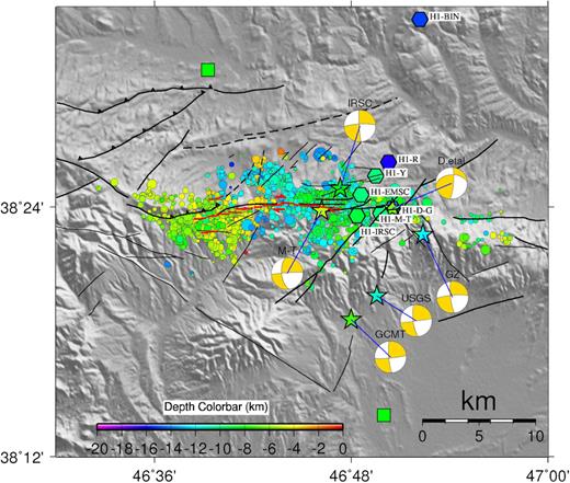
Locations of 2516 accurately located aftershocks (coloured circles, Momeni & Tatar 2018) and the M1 hypocentres and centroid focal mechanisms by previous studies. The aftershocks are recorded in ≥ 10 stations and have location error of <2 km and traveltime rms of <0.2 s (after Momeni & Tatar 2018). The hypocentres and centroid locations of M1 reported by international agencies and previous studies are shown by black hexagons and stars, respectively. H1-IRSC, H1-EMSC and H1-BIN are M1 hypocentres reported by IRSC, EMSC and BIN agencies, respectively. H1-D-G is M1 hypocentre by Donner et al. (2015) and Ghods et al. (2015). H1-R, H1-Y and H1-M-T are M1 hypocentres by Rezapour (2016), Yazdi et al. (2018) and Momeni & Tatar (2018) respectively. The centroid focal mechanism of each agency is labelled by their name on it and is connected to their corresponding centroid locations. The centroid focal mechanisms labelled D.etal and M-T are from Donner et al. (2015) and Momeni & Tatar (2018) studies respectively. The centroid focal mechanism labelled by GZ is from Geoazur. Inner colours represent the depths (after Momeni & Tatar 2018).
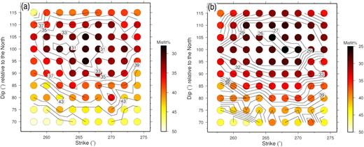
Correlation diagram between geometry and misfit of the M1 final rupture models that approximated using (a) one and (b) two elliptical slip patches in the inversion. Dip values of the fault planes are plotted relative to the north.
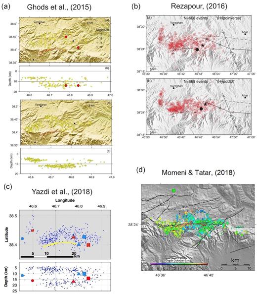
(a)–(d) The relocated aftershocks of the Ahar–Varzaghan seismic sequence by Ghods et al. (2015), Rezapour (2016), Yazdi et al. (2018) and Momeni & Tatar (2018) respectively. (a) Up: 184 selected M > 3 events from 2012 August 11 to November 07. They are located using local (comprised of three stations) and regional (permanent network) data. Down: 372 M > 2.5 aftershocks from 2012 August 13 to 24 using the local seismic network (comprised of three stations) alone. They have traveltime rms of <0.1 s and focal depth error of ≤3 km. (b) Up: distribution of 668 events relocated using HYPOINVERSE program and down: distribution of the same event using the hypoDD code. (c) Relocated aftershocks hypocentres (M ≥ 2.5) are shown with dots. The black square, triangle and circle respectively mark events with Mw = 6.4, 6.2 (August 11) and 5.6 (November 7). Same symbols in grey represent the calibrated hypocentres given by Ghods et al. (2015). For more information, see the cited papers. (d) 2516 relocated aftershocks during the first 24 d after the main shocks using data from a local dense seismic network (17 stations). The aftershocks were recorded in ≥10 stations and have location error of <2 km.
Parameters of 16 kinematic rupture models of M1 with one and two elliptical slip patches shown in Fig. 4.
| M1 | Main ellipse | Second ellipse | Both | ||||||||||||||
|---|---|---|---|---|---|---|---|---|---|---|---|---|---|---|---|---|---|
| Major | Minor | Slip | Vr | Rake | Tr | Mo. | Major | Minor | Slip | Vr | Rake | Tr | Mo. | T.M. | D | Misfit | |
| Model | (km) | (km) | (m) | (km s−1) | (deg) | (s) | N·m | (km) | (km) | (m) | (km s−1) | (deg) | (s) | N·m | N·m | (s) | (per cent) |
| 1 | 9.27 | 6.45 | 2.53 | 2.26 | 172.8 | 1.1 | 9.42E + 18 | – | – | – | – | – | – | – | 9.42E + 18 | 5.5 | 31 |
| 2 | 14.6 | 2.89 | 6.29 | 2.75 | 176.4 | 2.05 | 8.65E + 18 | – | – | – | – | – | – | – | 8.65E + 18 | 5.6 | 32 |
| 3 | 17.53 | 3.25 | 5.92 | 2.90 | 172.8 | 2.07 | 8.33E + 18 | – | – | – | – | – | – | – | 8.33E + 18 | 5.5 | 32 |
| 4 | 7.44 | 5.93 | 3.15 | 2.43 | 172.8 | 1.49 | 8.41E + 18 | – | – | – | – | – | – | – | 8.41E + 18 | 5.6 | 30 |
| 5 | 7.26 | 1.90 | 9.85 | 2.56 | 169 | 1.91 | 8.45E + 18 | – | – | – | – | – | – | – | 8.45E + 18 | 5.2 | 29 |
| 6 | 9.05 | 7.06 | 2.40 | 2.65 | 176.4 | 1.63 | 9.09E + 18 | – | – | – | – | – | – | – | 9.09E + 18 | 5.1 | 31 |
| 7 | 10.36 | 3.20 | 5.78 | 2.63 | 176.4 | 1.99 | 8.92E + 18 | – | – | – | – | – | – | – | 8.92E + 18 | 5.5 | 32 |
| 8 | 14.60 | 7.71 | 2.27 | 3.04 | 176.4 | 2.00 | 9.60E + 18 | – | – | – | – | – | – | – | 9.60E + 18 | 5.1 | 32 |
| 9 | 5.59 | 2.73 | 6.82 | 2.72 | 176.4 | 1.85 | 6.19E + 18 | 6.14 | 2.03 | 1.74 | 2.17 | 115.2 | 0.46 | 9.8E + 17 | 7.17E + 18 | 4.9 | 26 |
| 10 | 6.12 | 5.50 | 2.5 | 2.61 | 180 | 1.80 | 5.06E + 18 | 24.30 | 9.52 | 1.23 | 2.97 | 90 | 1.94 | 4.71E + 18 | 9.77E + 18 | 8 | 25 |
| 11 | 5.27 | 4.40 | 4.71 | 2.21 | 169.2 | 1.48 | 6.69E + 18 | 14.76 | 2.43 | 0.78 | 3.90 | 180 | 1.82 | 9.16E + 17 | 7.57E + 18 | 5.2 | 27 |
| 12 | 5.87 | 4.44 | 4.11 | 2.59 | 169.2 | 1.65 | 6.66E + 18 | 4.5 | 1.78 | 1.6 | 3.1 | 154.8 | 1.6 | 0.80E + 18 | 7.42E + 18 | 5.1 | 27 |
| 13 | 6.56 | 3.05 | 5.85 | 2.69 | 172.8 | 1.90 | 5.87E + 18 | 2.38 | 2.38 | 1.77 | 2.28 | 90 | 4.7 | 1.35E + 18 | 7.18E + 18 | 4.8 | 26 |
| 14 | 5.91 | 3.65 | 5.12 | 2.66 | 169.2 | 1.76 | 6.88E + 18 | 7.15 | 5.95 | 0.38 | 3.91 | 172.8 | 1.64 | 6.86E + 17 | 7.42E + 18 | 5.0 | 27 |
| 15 | 5.79 | 5.55 | 3.56 | 2.45 | 172.8 | 1.46 | 6.85E + 18 | 15.12 | 1.33 | 0.77 | 2.51 | 169.2 | 0.10 | 3.47E + 17 | 7.35E + 18 | 5.2 | 27 |
| 16 | 6.58 | 1.88 | 10.04 | 2.72 | 169.2 | 2.03 | 7.44E + 18 | 1.55 | 1.22 | 5.44 | 3.02 | 90 | 4.87 | 6.44E + 17 | 7.98E + 18 | 4.9 | 28 |
Notes: The wave fit of each final model and the convergence of their parameters are provided in the Supporting Information (Figs S1–S16). Major and minor: the semimajor and the semiminor axes of ellipse poles, respectively, slip: the maximum slip at the centre of each ellipse, Vr: the rupture velocity inside each ellipse, rake: the constant rake within each ellipse, Tr: the onset time, Mo: the seismic moment of each ellipse, T.M.: total seismic moment of each model, D: rupture duration of each model and misfit: the corresponding misfit of each model.
APPENDIX B: HYPOCENTRE AND GEOMETRY OF M2 SOURCE MODEL
Fig. B1 shows the hypocentre and centroid locations of M2 in previous studies. Our preferred hypocentre is the one of Momeni & Tatar (2018) which is relocated using the new local velocity model of the area (Table 2) obtained from precisely located aftershocks. Figs B2(a) and (b) show the correlation diagram between trial geometries of the M2 causative fault plane in the inversion using the preferred hypocentre and one and two elliptical slip patches, respectively. We observe on Fig. B2(a) that the trial M1 fault geometries with strikes ranging from 250° to 270° and a dip that ranges from 50° (N) to 72° (N) provide the best-fitting models with the misfit of ∼36–38 per cent when using one ellipse. Four of these models which are calculated on different geometries are shown in Fig. B3 (numbers 1–4).
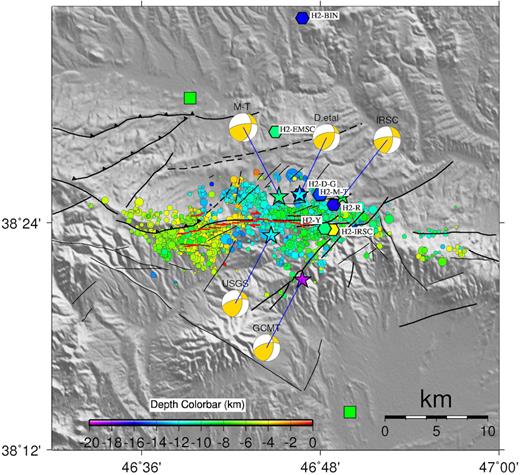
Locations of 2516 accurately located aftershocks (coloured circles, Momeni & Tatar 2018) and the M2 hypocentres and centroid focal mechanisms. The aftershocks are the same to Fig. A1. The hypocentres and centroid locations of M2 reported by international agencies and previous studies are shown by black hexagons and stars, respectively. H2-IRSC, H2-EMSC and H2-BIN are M2 hypocentres reported by IRSC, EMSC and BIN agencies, respectively. H2-D-G is M2 hypocentre by Donner et al. (2015) and Ghods et al. (2015). H2-R, H2-Y and H2-M-T are M2 hypocentres by Rezapour (2016), Yazdi et al. (2018) and Momeni & Tatar (2018), respectively. The centroid focal mechanism of each agency is labelled by their name on it and is connected to its corresponding centroid location. The centroid focal mechanisms labelled D.etal and M-T are from Donner et al. (2015) and Momeni & Tatar (2018) studies respectively. Inner colours represent the depths (after Momeni & Tatar 2018).
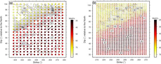
Correlation diagram between geometry and wave misfit (coloured contours) of M2 final kinematic rupture models using (a) one and (b) two elliptical slip patches in the inversion.
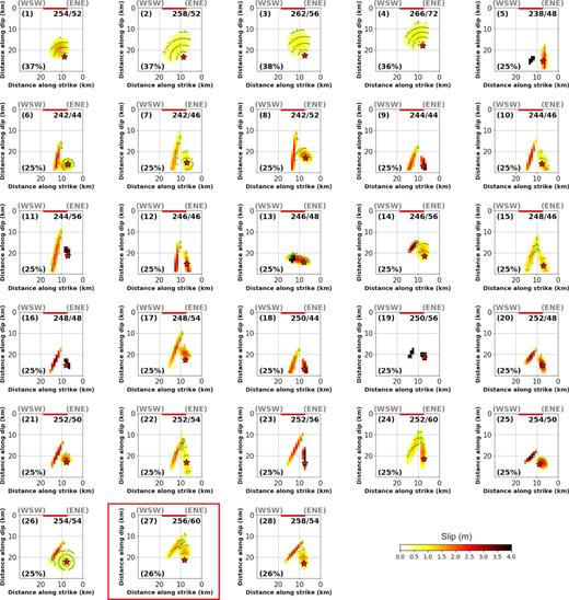
28 kinematic rupture models of M2 calculated by inverting near-field strong motion displacement time histories on different fault plane geometries and using one and two elliptical slip patches. Their source parameters are listed in Table B1. Each subfigure is labelled with a number on the left top. The geometry of each model is presented as (strike/dip) on the right-top of each subfigure. The fault dimension is in kilometres. The X-axis show distance along the strike and Y-axis is along downdip. The misfit of each model is written on the left bottom of each subfigure. The star is the earthquake hypocentre. Curved lines are positions of rupture front in time (seconds) after the origin time. Solid lines are positions of the reported surface rupture. The slip is saturated at 4 m.
When using two ellipses, the wave misfit of the resulting models is lower down to 25 per cent, and this is on strikes ranging from 235° to 260° and dips ranging from 40° to 65° (Fig. B2b). 24 of the two ellipses models of M2 which are calculated on different geometries are shown in Fig. B3 (numbers 5–28). About 11–13 per cent reduction of the misfit and the observed improvement it the waveform fit confirm the existence of two slip patches during M2 rupture.
The M2 source models that are calculated on fault planes with strikes <250° and dips <50° release scalar seismic moments of >3.7E + 18 up to 4.9E + 18 N·m. Also, their centroid depths are located roughly at ∼13 down to ∼16 km (Fig. B3 and Table B1). This information is inconsistent with the reported scalar seismic moment and centroid depth of the M2 from moment tensor inversion results using regional waveforms (3.2E + 18 N·m and 11 km, respectively, Momeni & Tatar 2018). Also, the models calculated on these geometries show some slip happening at depths deeper than M2 hypocentre (16.5 km). While the cut-off of precisely located aftershocks using a local seismic network data was reported at depth of ∼15 km (Fig. 8). So the probability that some slip could happen deeper than M2 hypocentre is low. The range of strikes between 252° and 260° and dips from 55° to 65°, for the M2 geometry, are the most consistent with the aftershocks distribution and with the moment tensor inversion results. We choose strike/dip = 256°/60° as our preferred geometry of M2 with ± 4° and ± 5° errors on strike and dip, respectively. This geometry is within the ranges that provide the minimum misfit for both one and two elliptical patches models (Figs B2a and b). It is also close to the almost EW striking nodal plane of the GCMT focal mechanism (strike/dip/rake = 255°/63°/134°) (Fig. B1), and also the same to the observed dip of lineated aftershocks (∼65° northward) in the same area (Momeni & Tatar 2018).
Parameters of the 28 M2 kinematic rupture models with one and two elliptical slip patches shown in Fig. B3.
| M2 | Geometry | Ellipse-1 (eastern) | Ellipse-2 (western) | Total | ||||||||||||||
|---|---|---|---|---|---|---|---|---|---|---|---|---|---|---|---|---|---|---|
| Strike/dip | Major | Minor | Slip | Vr | Rake | Tr | Mo. | Major | Minor | Slip | Vr | Rake | Tr | Mo. | Mo. | T | Misfit | |
| Model | (°/°) | (km) | (km) | (m) | (km s−1) | (°) | (s) | N·m | (km) | (km) | (m) | (km s−1) | (°) | (s) | N·m | N·m | (s) | (per cent) |
| 1 | 254/52 | 5.41 | 4.32 | 1.72 | 2.46 | 137 | 1.09 | 3.00E + 18 | – | – | – | – | – | – | – | 3.00E + 18 | 4 | 37 |
| 2 | 258/52 | 8.60 | 5.48 | 0.90 | 3.11 | 144 | 1.15 | 3.15E + 18 | – | – | – | – | – | – | – | 3.15E + 18 | 4.1 | 37 |
| 3 | 262/56 | 6.76 | 5.8 | 1.01 | 3.15 | 140 | 1.16 | 2.93E + 18 | – | – | – | – | – | – | – | 2.93E + 18 | 4.2 | 38 |
| 4 | 266/72 | 7.21 | 5.33 | 1.06 | 2.3 | 133 | 0.44 | 2.95E + 18 | – | – | – | – | – | – | – | 2.95E + 18 | 5.1 | 36 |
| 5 | 238/48 | 8.38 | 1.27 | 2.61 | 3.54 | 180 | 1.57 | 1.74 E + 18 | 2.499 | 1.05 | 8.89 | 2.31 | 112 | 0.63 | 2.10E + 18 | 3.72E + 18 | 5.1 | 27.7 |
| 6 | 242/44 | 4.48 | 3.43 | 1.60 | 1.47 | 176 | 0.36 | 1.88E + 18 | 8.36 | 1.16 | 2.56 | 2.15 | 0.286 | 0.11 | 1.89E + 18 | 3.77E + 18 | 5.2 | 25 |
| 7 | 242/46 | 8.67 | 2.69 | 1.27 | 2.83 | 180 | 1.22 | 1.67E + 18 | 15.72 | 1.44 | 1.85 | 2.57 | 0.31 112 | 0.28 | 2.34E + 18 | 4.01E + 18 | 5.3 | 25 |
| 8 | 242/52 | 4.52 | 3.10 | 1.92 | 2.71 | 180 | 1.38 | 2.05E + 18 | 14.02 | 1.04 | 2.69 | 2.61 | 0.28 104 | 0.39 | 2.39E + 18 | 4.44E + 18 | 5.2 | 25 |
| 9 | 244/44 | 6.32 | 1.18 | 4.07 | 3.12 | 180 | 1.72 | 1.80 E + 18 | 10.07 | 1.41 | 2.36 | 2.37 | 0.32 115 | 0.21 | 1.92E + 18 | 3.67E + 18 | 4.2 | 25 |
| 10 | 244/46 | 11.95 | 2.09 | 1.72 | 3.19 | 180 | 1.33 | 1.68 E + 18 | 8.98 | 1.06 | 2.84 | 2.61 | 0.31 112 | 0.48 | 2.00E + 18 | 3.74E + 18 | 4.2 | 25 |
| 11 | 244/56 | 2.57 | 1.38 | 6.72 | 2.65 | 180 | 1.53 | 1.81 E + 18 | 14.49 | 1.36 | 2.32 | 2.44 | 0.29 104 | 0.38 | 3.25E + 18 | 4.92E + 18 | 5.2 | 25 |
| 12 | 246/46 | 13.19 | 1.61 | 2.60 | 2.93 | 180 | 1.15 | 1.66 E + 18 | 13.49 | 1.14 | 3.02 | 2.2 | 0.31 112 | 0.50 | 2.28E + 18 | 4.06E + 18 | 5.1 | 25 |
| 13 | 246/48 | 6.18 | 2.47 | 2.66 | 1.39 | 180 | 0.10 | 3.18 E + 18 | 1.81 | 1.12 | 6.37 | 2.28 | 0.29 104 | 0.89 | 1.15E + 18 | 4.22E + 18 | 5.2 | 26 |
| 14 | 246/56 | 2.61 | 1.92 | 4.57 | 1.17 | 176 | 0.10 | 1.64 E + 18 | 7.22 | 1.19 | 2.94 | 2.19 | 0.29 104 | 0.23 | 2.03E + 18 | 3.77E + 18 | 5.1 | 25 |
| 15 | 248/46 | 12.49 | 1.93 | 1.54 | 3.97 | 180 | 1.57 | 1.60 E + 18 | 11.78 | 1.57 | 1.61 | 2.67 | 0.32115 | 0.12 | 2.07E + 18 | 3.83E + 18 | 5.2 | 25 |
| 16 | 248/48 | 2.94 | 1.08 | 8.25 | 3.02 | 180 | 1.76 | 2.05 E + 18 | 6.28 | 1.76 | 3.94 | 2.32 | 0.32 115 | 0.55 | 1.82E + 18 | 3.79E + 18 | 4.0 | 25 |
| 17 | 248/54 | 3.72 | 2.56 | 2.39 | 3.66 | 180 | 1.63 | 1.97 E + 18 | 10.55 | 1.21 | 2.25 | 2.60 | 108 | 0.46 | 2.18E + 18 | 3.89E + 18 | 5.2 | 24 |
| 18 | 250/44 | 6.34 | 1.17 | 4.07 | 3.12 | 180 | 1.72 | 1.80 E + 18 | 10.07 | 1.41 | 2.34 | 2.37 | 0.32 115 | 0.21 | 1.92E + 18 | 3.71E + 18 | 4.1 | 25 |
| 19 | 250/56 | 2.17 | 1.30 | 8.39 | 2.35 | 180 | 1.60 | 1.81 E + 18 | 1.60 | 1.07 | 8.09 | 2.79 | 0.31 104 | 0.89 | 3.25E + 18 | 3.67E + 18 | 5.0 | 25 |
| 20 | 252/48 | 4.70 | 1.61 | 2.88 | 2.51 | 180 | 1.5 | 1.87 E + 18 | 4.59 | 1.28 | 3.43 | 2.35 | 0.34 | 0.22 | 1.94E + 18 | 3.24E + 18 | 4.3 | 26 |
| 21 | 252/50 | 3.05 | 2.83 | 2.27 | 2.23 | 180 | 1.38 | 1.55 E + 18 | 7.25 | 1.00 | 3.41 | 2.0 | 115 | 0.11 | 1.79E + 18 | 3.29E + 18 | 4.8 | 25 |
| 22 | 252/54 | 17.86 | 1.89 | 1.22 | 3.94 | 180 | 1.33 | 1.88 E + 18 | 8.35 | 1.26 | 2.18 | 2.48 | 0.31 112 | 0.36 | 1.77E + 18 | 3.78E + 18 | 5.1 | 25 |
| 23 | 252/56 | 6.01 | 1.00 | 4.84 | 3.26 | 176 | 1.70 | 1.97 E + 18 | 9.30 | 1.04 | 2.69 | 2.61 | 0.30 108 | 0.51 | 1.87E + 18 | 3.84E + 18 | 5.1 | 25 |
| 24 | 252/60 | 7.38 | 1.56 | 2.06 | 3.78 | 180 | 1.54 | 1.79 E + 18 | 9.45 | 2.05 | 1.43 | 2.66 | 108 | 0.30 | 2.08E + 18 | 3.75E + 18 | 5.2 | 25 |
| 25 | 254/50 | 3.31 | 2.74 | 2. 67 | 3.62 | 180 | 1.75 | 1.78 E + 18 | 1.14 | 1.13 | 4.5 | 2.20 | 122 | 0.46 | 1.60E + 18 | 3.41E + 18 | 3.4 | 26 |
| 26 | 254/54 | 6.20 | 5.74 | 0.82 | 1.84 | 176 | 0.49 | 2.18E + 18 | 6.56 | 1.00 | 2.48 | 2.25 | 0.31 | 0.23 | 1.24E + 18 | 3.42E + 18 | 4.2 | 27 |
| 27 | 256/60 | 4.66 | 2.87 | 1.58 | 3.75 | 180 | 1.62 | 1.60 E + 18 | 7.53 | 1.81 | 1.67 | 2.48 | 112 | 0.14 | 1.74E + 18 | 3.29E + 18 | 5.1 | 26 |
| 28 | 258/54 | 5.43 | 2.34 | 1.73 | 3.68 | 180 | 1.81 | 1.63 E + 18 | 7.29 | 1.00 | 2.87 | 2.57 | 122 | 0.33 | 1.62E + 18 | 3.25E + 18 | 4.1 | 26 |
Notes: The fault geometry (strike/dip) of each model is presented in the ‘strike/dip’ column. Notations are same as Table A1.
Parameters of the 16 M2 kinematic rupture models with one and two elliptical slip patches shown in Fig. 5.
| M2 | Ellipse-1 (eastern) | Ellipse-2 (western) | Total | ||||||||||||||
|---|---|---|---|---|---|---|---|---|---|---|---|---|---|---|---|---|---|
| Major | Minor | Slip | Vr | Rake | Tr | Mo. | Major | Minor | Slip | Vr | Rake | Tr | Mo. | Mo. | T | Misfit | |
| Model | (km) | (km) | (m) | (km s−1) | (°) | (s) | N·m | (km) | (km) | (m) | (km s−1) | (°) | (s) | N·m | N·m | (s) | (per cent) |
| 1 | 5.15 | 1.45 | 5.34 | 2.6 | 137 | 1.34 | 3.02E + 18 | – | – | – | – | – | – | – | 3.02E + 18 | 3.9 | 39 |
| 2 | 5.18 | 1.30 | 6.03 | 2.27 | 130 | 1.21 | 2.98E + 18 | – | – | – | – | – | – | – | 2.98E + 18 | 4.4 | 38 |
| 3 | 5.51 | 3.98 | 1.83 | 2.31 | 137 | 0.97 | 3.03E + 18 | – | – | – | – | – | – | – | 3.03E + 18 | 4.2 | 37 |
| 4 | 5.15 | 1.00 | 9.88 | 2.72 | 140 | 1.7 | 3.49E + 18 | – | – | – | – | – | – | – | 3.49E + 18 | 3.3 | 39 |
| 5 | 11.37 | 4.5 | 0.92 | 2.84 | 140 | 1.19 | 3.44 E + 18 | – | – | – | – | – | – | – | 3.44 E + 18 | 4.4 | 36 |
| 6 | 5.43 | 4.87 | 1.56 | 2.64 | 137 | 1.23 | 3.05E + 18 | – | – | – | – | – | – | – | 3.05E + 18 | 4.1 | 37 |
| 7 | 5.65 | 1.6 | 4.41 | 2.41 | 130 | 1.25 | 2.83E + 18 | – | – | – | – | – | – | – | 2.83E + 18 | 4.6 | 38 |
| 8 | 10.06 | 3.32 | 1.23 | 3.92 | 130 | 1.97 | 2.91E + 18 | – | – | – | – | – | – | – | 2.91E + 18 | 4.4 | 38 |
| 9 | 4.65 | 2.87 | 1.59 | 3.75 | 180 | 1.62 | 1.55E + 18 | 7.52 | 1.81 | 1.67 | 2.48 | 115 | 1.43 | 1.74E + 18 | 3.29E + 18 | 5.1 | 26 |
| 10 | 8.08 | 2.04 | 2.02 | 3.48 | 176 | 1.79 | 2.05E + 18 | 7.56 | 2.30 | 1.0 | 2.70 | 112 | 0.48 | 1.71 E + 18 | 3.76E + 18 | 5.1 | 27 |
| 11 | 6.75 | 5.62 | 0.88 | 2.92 | 172 | 1.39 | 2.54E + 18 | 7.75 | 1.63 | 1.40 | 2.4 | 104 | 0.33 | 1.27 E + 18 | 3.81E + 18 | 5.2 | 26 |
| 12 | 10.3 | 1.02 | 2.41 | 3.19 | 176 | 1.42 | 1.74E + 18 | 6.97 | 1.31 | 2.47 | 2.21 | 108 | 0.50 | 1.67 E + 18 | 3.41E + 18 | 5.1 | 26 |
| 13 | 5.52 | 2.04 | 1.98 | 2.82 | 173 | 1.41 | 1.66E + 18 | 7.23 | 1.43 | 2.03 | 2.48 | 110 | 1.79 | 1.58 E + 18 | 3.24E + 18 | 5.1 | 26 |
| 14 | 3.47 | 2.67 | 2.65 | 2.69 | 180 | 1.54 | 1.87E + 18 | 10.35 | 1.03 | 2.61 | 2.39 | 108 | 0.42 | 2.02E + 18 | 3.89E + 18 | 5.1 | 26 |
| 15 | 9.53 | 2.43 | 0.98 | 3.99 | 175 | 1.6 | 1.72E + 18 | 8.19 | 1.56 | 1.61 | 2.81 | 115 | 0.27 | 1.52 E + 18 | 3.24E + 18 | 4.5 | 26 |
| 16 | 8.71 | 1.92 | 1.50 | 3.78 | 177 | 1.74 | 1.91E + 18 | 7.40 | 1.29 | 2.31 | 2.49 | 108 | 0.59 | 1.63 E + 18 | 3.54E + 18 | 4.6 | 26 |
Notes: The models are calculated on the preferred geometry with strike/dip = 256°/60°. Notations are same as Table A1.
The proposed M2 geometries by Alipour (2013), Donner et al. (2015), Zafarani et al. (2015), Yadav et al. (2016), Yazdi et al. (2018) and Amini et al. (2018) are not in our accepted range of geometries. While the suggested M2 geometries by Ghods et al. (2015), Rezapour (2016) and Momeni & Tatar (2018) are in the accepted range.
