


SUMMARY
We propose a new Bayesian method to reveal the Vs structure of the near surface of the earth using spatial autocorrelation (SPAC) functions and apply this new method to synthetic, broad-band and geophone data sets. The principle of SPAC is introduced, and an implementation of the Bayesian Monte Carlo inversion (BMCI) for modelling SPAC coherency functions is described. To demonstrate its effectiveness, BMCI is applied to synthetic tests, data from 14 SPAC array sites in the Salt Lake Valley (SLV), Utah, and two arrays (one broad-band and one geophone) located in south central Utah. The Vs models derived from previous SPAC analysis of the 14 SLV sites differ by 10 per cent at most from those determined by BMCI and lie within uncertainties determined for the BMCI models. These agreements demonstrate the effectiveness of the BMCI method. The synthetic tests and applications to the SLV SPAC data show BMCI has great potential to resolve Vs structure down to at least 400 m. To achieve resolution for deeper Vs structure, longer duration deployments, wider array apertures, and additional seismometers or geophones can be used. Additionally, when the target frequencies are greater than 0.1 Hz, there is no apparent disadvantage in using geophone data for BMCI compared to broad-band data. Most significantly, BMCI places a quantifiable constraint on the uncertainties of the Vs models as well as Vs30.
1 INTRODUCTION
Spatial autocorrelation (SPAC), the cross-correlation of ambient noise in the frequency domain, is based on the theory that ambient noise wave propagation can be treated as a stationary stochastic process in time and space (Aki 1957). In current practice, SPAC functions are generated from vertical-component data and Rayleigh wave dispersion curves are extracted from the SPAC functions to invert for near-surface shear velocity (Vs) structure (Bettig et al.2001; Okada 2003; Cho et al.2004; Chavez-Garcia et al.2006; Di Giulio et al.2006; Picozzi & Albarello 2007). SPAC approaches are roughly equivalent to the widely used time-domain ambient noise methods (e.g. Tsai & Moschetti 2010). However, where time-domain analyses are widely used to resolve regional or global Vs structure (e.g. Bensen et al.2007; Ekstrom et al.2009; Lin et al. 2013), SPAC is typically used in geotechnical engineering studies to characterize shallow Vs structure like Vs30, the average shear wave velocity of the upper 30 m. Vs30 is used to characterize ground motion amplification due to site effects (Borcherdt 1994).
In typical SPAC experiments, broad-band instruments are deployed in arrays with regular spacing, such as equilateral triangles (Fig. 1, inset). The noise source is assumed to be random and homogeneous in both space and time, and generates an omnidirectional wavefield, in which microtremors are a spatiotemporal stochastic process (Okada 2003). The coherency curves (cross-correlation functions of data in the frequency domain for station pairs) from stations with equal spacing can be stacked to enhance signal. These experiments often use a limited number of instruments deployed at each array dimension for a relatively short-time period (2–4 hr). The array dimension and time period of recording are often limited by the availability of small pools of appropriate instruments. To determine the velocity structure using SPAC, studies use forward modelling to manually change shear-wave velocities and thicknesses of layers in direct-fitting methodologies (e.g. Asten et al 2004; Wathelet et al.2005; Asten 2006; Stephenson & Odum 2010) or by extracting phase-velocity dispersion data that are then inverted for a layered-earth model (e.g. Di Giulio et al.2006; Picozzi & Albarello 2007).
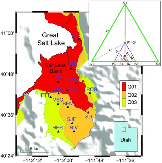
Distribution of 14 SPAC campaigns (triangles) in Salt Lake Basin, Utah. These campaigns are located in three geological Quaternary surficial units, Q01, Q02 and Q03 (youngest to oldest). Inset, station geometry of a SPAC campaign, composed of three triangles (inner thin, middle dashed and outer thick). Each triangle subarray is composed of three stations at the vertices and one at the centre (stars).
Recently, SPAC methodologies have been evolving to include three-component wavefield analysis (Köhler et al.2007; Lamb et al.2014) and nontraditional array designs (Cho et al.2004; Chavez-Garcia et al.2006). In this study, we propose two additional adaptations. First, we present a novel Bayesian approach to reveal shallow Vs structure by directly fitting SPAC functions in the coherency domain rather than through inversion of picked dispersion data. In this method, a Bayesian Monte Carlo inversion (BMCI) is used for direct fitting in the coherency domain (cross-power coherence). The BMCI is based on the Bayesian theorem and uses repeated random sampling in the model space to get the statistical properties of the Vs structure. This type of Bayesian approach has been applied in other studies using fundamental mode surface waves in the time domain to resolve the shear velocity by inverting the phase velocities from ambient noise tomography (Shapiro & Ritzwoller 2002; Bodin & Sambridge 2009; Shen et al.2013) and from the spectral analysis of surface waves (SASW) and H/V data (Teague & Cox 2016). Using BMCI is not only a more robust method for determining the global minima, it also provides a means for quantifying uncertainty in the resulting models.
In the second adaptation, we test the capabilities of using 5-Hz geophones in resolving the shear wave velocity structure at depths shallower than ∼300 m. These instruments are now commonly used for time-domain ambient noise tomography studies (e.g. Lin et al.2013; Wang et al.2017; Wu et al.2017), and here we test whether they can be used for SPAC. While these instruments have a limited bandwidth and sensitivity compared to broad-band instruments, large numbers of such instruments could be used to extend both the duration and aperture of SPAC experiments.
The paper is organized as follows. First, we introduce the principles of SPAC as well as BMCI and develop a BMCI workflow as described by the flowchart in Fig. 2. Next, to validate this new Bayesian SPAC approach, we compare results using the same data and the new method to results determined using multimode SPAC (MMSPAC) for 14 sites in the Salt Lake Valley (SLV), Utah (Stephenson & Odum 2010). Finally, to further investigate the feasibility of using portable geophone arrays, we compare the SPAC functions and Vs results determined using the new BMCI approach at two nearby sites: in one the data were collected using a four-element broad-band array and in the other data were collected using a ten-element geophone array.

2 METHODOLOGY
2.1 Principle of SPAC
2.2 Markov chain Monte Carlo method—Metropolis Hastings algorithm
Model |${m_i}$| is replaced by model |${m_{i - 1}}$| if model |${m_i}$| is rejected; otherwise, it is accepted into the model pool used to get the final model. The process is continued using N iterations (Fig. 2). For this study, N equals 3000.
Once N models are derived from the model space, the posterior distribution can be described as follows. As the model converges, it is common to get several repeated models in the model pool. To make the Markov Chain reach the equilibrium distribution, we discard half of the derived models; this means that |$N/2$| is taken as the burn-in point. The remaining models are subject to the posterior distribution of the model space as described in eq. (3). To further optimize the solution, the 1000 best Vs models in the remaining pool are averaged at every 0.3 meters to achieve the final Vs model. The uncertainty of the final model is then defined by the standard derivation of the 1000 best models.
2.3 Validation of BMCI using synthetic data
To validate the effectiveness of BMCI, two synthetic tests with an array configuration as shown in the Inset of Fig. 1 are performed, as illustrated in Fig. 3. In this study, the coherency functions have high signal-to-noise ratios for frequencies greater than 2 Hz (|${f_{min}}$|). Using equation |${D_{max}} = V/( {{a_{max}}{f_{min}}} )\ $| proposed by Asten & Hayashi (2018) with an average phase velocity V of 1200 m s–1 and a constant |${a_{max}}$| of 2 indicates that Vs structure can be resolved for depths less than 300 m (|${D_{max}}$|). This depth range is represented by the shallowest five layers of the true model used in the two following synthetic tests (Table S1). Because the deeper Vs structure is not resolved, we fixed the parameters for the two deepest layers without any impact to the solution of BMCI. We generated three sets of SPAC coherency functions following Okada (2003), which assumes an omnidirectional wavefield, with different levels of Gaussian white noise, which are described by the standard deviations of the zero-mean normal distribution: 0, 0.05 and 0.2, respectively.
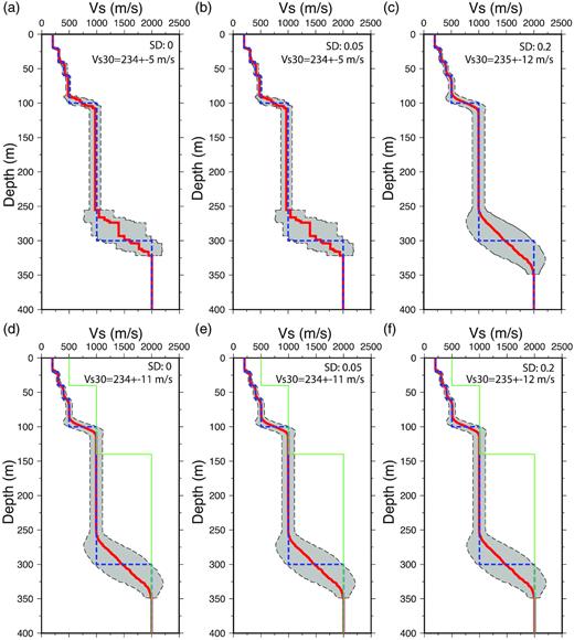
Resultant Vs models with uncertainty areas characterized by |$1\sigma $| standard deviation (grey area) for three noise levels: (a) 0.0, (b) 0.05 and (c) 0.2 for synthetic test 1 with the starting model being the true model (moderate dashed line), and average model (thick line): (d) 0.0, (e) 0.05 and (f) 0.2 for synthetic test 2 with the starting model (thin line) greatly differing from the true model (moderate dashed line). The average Vs profile is represented by the red thick line. The Vs30 for each case are annotated on the individual plots.
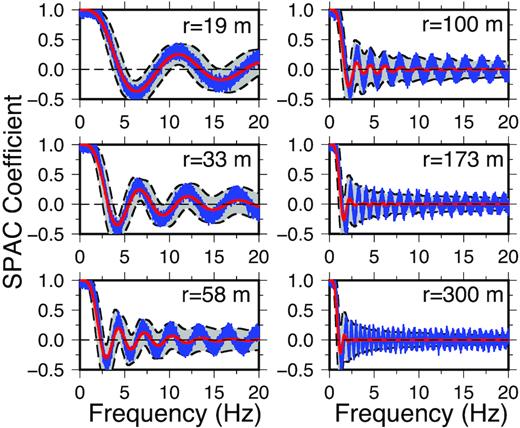
If there is a well-formed model |${m_0}$|, then we generate the model space by |${m_0} \pm 0.2{m_0}$|, following Shen et al. (2013) and Bassin et al. (2000). For regions without known velocity models, a much larger model space like that adopted in the synthetic test in the Discussion section can be provided. In this study, the Vs and thicknesses of the top five layers are the variables in the model as listed in Table S1. For the first synthetic test, the three data sets are inverted for the velocity models using BMCI (Figs 3a–c). Fits to the coherency functions are shown in Figs 4 and S1a. There are no substantial differences between the models and the Vs30 values for the tests with 0 and 0.05 noise levels (Figs 3a and b). However, the data set derived using a 0.2 noise level is not well fit (Fig. S1a) and errors on Vs30 are twice that observed for the other noise levels (Figs 3a–c). For longer interstation spacings like 173 and 300 m, amplitudes of the averaged, synthesized coherency functions for higher frequencies decrease with noise level due to decrease of the similarity of the coherency functions, indicating that the noise level in the coherency functions has a stronger effect at longer interstation spacings. One way to decrease overall noise levels is to stack coherency functions over long time intervals. From the synthetic results, it seems that to get high-quality coherency functions for longer interstation spacings acquisition with longer duration may be required. This is most clearly seen for 0.2 noise level at 300 m where the coherency drops to zero at frequencies above 3 Hz (Fig. S1a).
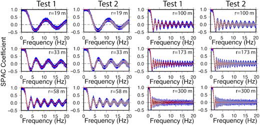
Coherency function fits for synthetic tests 1 and 2 in an omnidirectional wavefield with a noise level of 0.05. The coherency fits for noise levels of 0.0 and 0.2 for the two tests are shown in Figs S1a and S1b, respectively. Moderate lines indicate the average coherency functions from the posterior velocity models. 2σ of the coherency functions are presented by grey areas outlined by dashed lines, and black thin lines are the summation of the coherency functions predicted by the given model in Fig. 3.
The BMCI is relatively insensitive to the initial model. To demonstrate this, a second synthetic test is carried out. The only difference between the two tests is that test 2 uses an initial model dramatically different from the true model (Figs 3d–f). Although the initial model is substantially different than the true model, the velocity models derived from BMCI converge to the true model for all the three noise levels (Figs 3d–f), the Vs30 values converge to the true value of 233 m s–1, and the uncertainties for the three noise levels are nearly the same as determined in the first test. Moreover, the averaged coherency functions overall fit the synthesized data well (Figs 4 and S1b). However, amplitudes of the averaged, synthesized coherency functions at the interstation spacings 173 and 300 m decrease for higher frequencies, indicating that the initial model has an effect at longer interstation spacings.
With high-quality data like those in the synthetic tests, BMCI can resolve the Vs structure down to 300 m (Fig. 3). However, the Vs gradually increases from 1000 to 2000 m s–1 instead of resolving the velocity step in the true model. This is due to averaging 1000 Vs models with similar structures to the true model (Table S1), which smears velocity steps into gradients, indicating uncertainties of the interface depths. Despite smoothing of the deeper Vs structure, the two synthetic tests show that BMCI has the potential to resolve the deeper Vs structure.
The two synthetic tests demonstrate the effectiveness of BMCI. First, the resultant models determined by BMCI reasonably match the true model (moderate dashed lines in Fig. 3), though the resultant models are smoothed due to averaging. Second, the synthetic coherency functions generated by the resultant models perfectly fit the coherency functions from the given model; this holds even for the noisiest data set (Figs 4, and S1a–S1b). Third, both the true Vs30 (300 m s–1) and Vs100 (380 m s–1) are recovered within the confidence bounds. Fourth, as demonstrated above, BMCI is insensitive to the initial model. Additionally, the success of the application of the BMCI to the noisiest SPAC data shows that even with noisy data, BMCI recovers a good approximation of the true model.
3 SALT LAKE VALLEY SPAC DATA
To assess seismic hazards to the Salt Lake Valley, an urban region located atop a fault-bounded sedimentary basin, Stephenson & Odum (2010) acquired microtremor array data at 14 sites (Fig. 1) to determine the shallow Vs structure using MMSPAC (Asten 2006). For each experiment, four stations were deployed in three triangles for a duration of 30 min (Inset of Fig. 1). For each triangle, there are two distances: |$a/\sqrt 3 $| and a. The edge lengths (a) of the three triangles are ∼33.3, ∼100 and ∼300 m, respectively, with corresponding radial interstation spacings of ∼19.2, ∼57.7 and ∼173.2 m. Since all the SLV sites are located in a downtown urban area, an omnidirectional noise wavefield is expected (Asten 2006).
The shallow Salt Lake Basin is composed primarily of Quaternary sediments whose thickness can locally be greater than 1 km (Mabey 1992). The 14 SPAC sites are located in three mapped Quaternary surficial units, Q01, Q02 and Q03 (youngest to oldest) (McDonald & Ashland 2008) as shown in Fig. 1. Specifically, there are five sites (CAM, FS, JRP, LP and RIC) in Q01, six sites (BEN, MAG, RIV, ROS, SJF and SD) in Q02, and three sites (HER, FTT and VEC) in Q03. The unit Q01 is characterized by lacustrine and alluvial clay, silt and fine sand, unit Q02 is dominated by a combination of sand and gravel, and unit Q03 is predominantly sand-to-gravel alluvial/lacustrine deposits. McDonald & Ashland (2008) found that the three units are characterized by statistically distinct Vs30 values: 194 m s–1 (151–325 m s–1), 281 m s–1 (206–469 m s–1) and 402 m s–1 (294–708 m s–1) for units Q01, Q02 and Q03, respectively.
Here, we reprocess the vertical component of these data to resolve the Vs profiles using the proposed BMCI method described in Section 2 and compare the new results to those derived by Stephenson & Odum (2010). The raw data were detrended, demeaned, filtered between 0.1 and 20 Hz, and synchronized in time for each triangular array. We chose the frequency band of 0–20 Hz to best compare to results of Stephenson & Odum (2010). The coherency curves are high quality and real and imaginary components are not in phase as shown in Figs S2a–S2c; this supports the argument that the noise wavefields near the SLV sites are omnidirectional. The imaginary part of the coherency curves typically has SDs less than 0.1 (Table S2). Next, the normalized spatial cross-spectrum is calculated for each station pair. For each interstation spacing, the three normalized individual spectra acquired on different azimuths were averaged to derive the observed SPAC coherency function. At each SLV site, initial models utilized in BMCI (thin lines in Fig. 5) are randomly generated from the model space, formed by |${m_t} \pm 0.2{m_t}$|, where |${m_t}$| are velocity models derived by Stephenson & Odum (2010) (moderate dashed lines in Fig. 5).
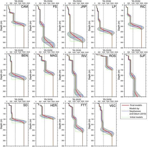
Vs profiles derived from BMCI for 14 SLV sites. The average profiles of the posterior Vs models are indicated by thick lines, and the |$1\sigma $| uncertainties of the Vs profiles are represented by grey areas. The models derived by Stephenson & Odum (2010) for the 14 SLV sites are denoted by moderate dashed lines, while the starting models for the inversion are indicated by thin lines.
4 RESULTS FROM SALT LAKE VALLEY BMCI MODELLING
After applying BMCI and inverting for the coherency functions, the Vs profiles at the 14 sites are obtained, as shown in Fig. 5. For most of the sites, the initial models, which are modified from the MMSPAC models (Stephenson & Odum 2010), are within 1|${\rm{\sigma }}$| of the average models. Considering an uncertainty of 10 per cent for the MMSPAC models estimated empirically by Stephenson & Odum (2010), the agreement between BMCI and MMSPAC results is very good. The predicted coherency functions typically fit the observations well (Figs 6 and S3a–S3c). It is noteworthy that the BMCI models smooth the shear-wave steps into gradients compared to the models derived by Stephenson & Odum (2010). This same tendency was seen in the synthetic tests and was found to be the result of averaging the 1000 best models. Importantly, the velocity gradients indicate the uncertainties of the interface depths.
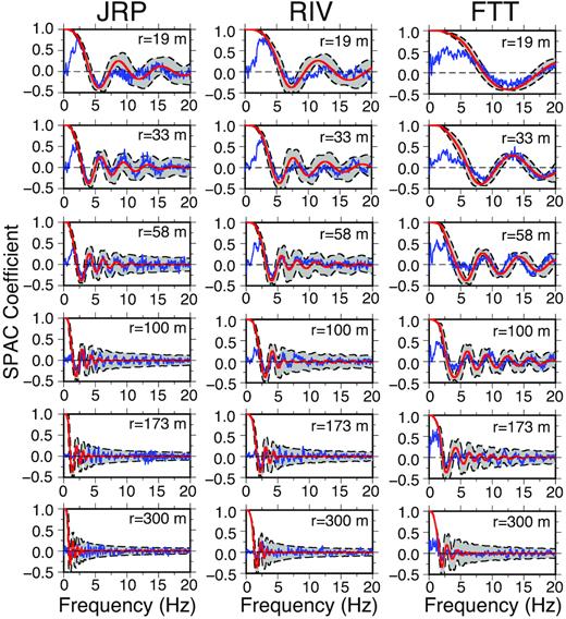
Coherency function fits for the sites JRP, RIV and FTT, and those for other SLV sites shown in Figs S3a–3c. Moderate curved lines indicate the averages coherency functions from the posterior velocity models. 2σ of the coherency functions are presented by grey areas behind the red and blue curved lines. Thin lines are the observations.
Unconsolidated sediments are loose accumulations of deposits with large porosities and shear wave velocities commonly less than 1000 m s–1 (Zimmer 2003; Lee 2010). Site FS located in Quaternary unit Q01, near the centre of the unit has thicker unconsolidated sediments or a deeper high Vs contrast, compared to the sites (CAM, LP and RIC) located near the edge of the mapped boundary (Fig. 7). However, site JRP, also located near the Q01 boundary has a thick layer of unconsolidated sediments (285 ± 48 m) similar to site FS. Since resolution decreases with depth, the bottom of the sedimentary layer may not be well-resolved due to lack of constraints from these SPAC data. Notably, the thick unconsolidated sediments at the site JRP are also present in the Wasatch community velocity model (WCVM; Magistrale et al.2009), which incorporates Vs30, gravity, and industry seismic reflection interpretations.
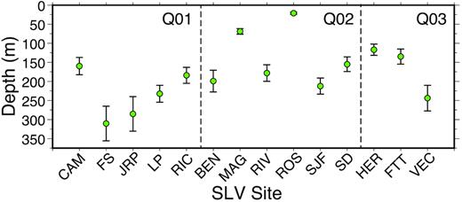
Thicknesses of the unconsolidated sediments at 14 SLV sites as defined by a velocity of 1000 m s–1. The error bars indicate |$1\sigma $| of the mean (dots). The 14 SLV sites are located in three Quaternary units Q01, Q02 and Q03, and are divided by the dashed lines.
For Quaternary unit Q02, sites BEN, RIV, and SJF in the centre of the unit have thicker unconsolidated sediments than sites MAG and ROS (Fig. 7). In particular, site ROS has the thinnest unconsolidated sediments at 22.5 m, which is not sufficiently thick to excite longer-period surface waves sensitive to deeper Vs structure. This leads to poor-quality coherence functions at interstation spacings of 173 and 300 m, as shown in Fig. S3b. Because of this, it is difficult to resolve structure below 60 m at this site based on the one-third wavelength rule (e.g. Asten & Hayashi 2018). There are only three sites in Quaternary unit Q03. Again, those located near the mountains at the edge of the SLV have thinner unconsolidated sediments that are ineffective at exciting longer-period surface waves, resulting in less useful coherency functions at the longer interstation spacings (Fig. S3c).
One direct demonstration of the effectiveness of BMCI used in the study is the comparison of Vs30s and Vs100s in this study and those derived by Stephenson & Odum (2010) at the same 14 SLV sites (Fig. 8). For all the sites, the Vs30s obtained by Stephenson & Odum (2010) are within |$2\sigma $| of those estimated by the BMCI, indicating there are no significant differences between the results from the two studies. For Vs100s, the results of all the sites in this study agree with those derived by Stephenson & Odum (2010) even for site ROS, where the poor-quality coherency functions at the longer distances led to less well-constrained Vs profiles at depths greater than 30 m. Overall, the good agreement of both Vs30 and Vs100 demonstrates the effectiveness of the BMCI method. More importantly, the results constrained by the BMCI have numerically quantified uncertainties (|$\sigma )$| relative to the empirically estimated uncertainty of many other SPAC methods, such as MMSPAC (Asten et al.2004; Asten 2006).
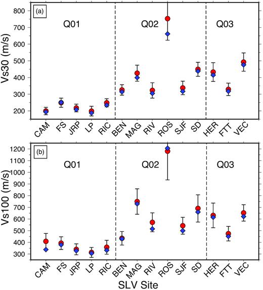
Comparison of (a) Vs30 and (b) Vs100 between those derived by BMCI in this study (red dots with error bars) and those derived by Stephenson & Odum (2010) (blue diamonds). The error bars are the ranges within 2σ of the mean (red dots). The 14 SLV sites are located in three Quaternary units Q01, Q02 and Q03, and are divided by the dashed lines. Note that the y-axis values for the two subfigures are different.
Besides the velocity models derived by Stephenson & Odum (2010), there are velocity models constrained by active source spectral-analysis-of-surface-wave (SASW, Wilder 2007) and minivib refraction and reflection (Stephenson et al.2007) nearby the sites BEN, FS, FTT, JRP, and LP. In the vicinities of the sites CAM and MAG the Vs structures are constrained with borehole logs (Williams et al.1993). Stephenson & Odum (2010) have done a comparison of their results with those previous analyses and found they have ∼10 per cent differences. The differences at the same level can also be seen in Vs30 comparison between Stephenson & Odum's (2010) and ours (Fig. 8a). This indicates that our results agree with those previous analyses as well.
The resultant Vs30s are also consistent with the average Vs30 for the Quaternary units Q01 (194 m s–1), Q02 (281 m s–1) and Q03 (402 m s–1) in the Salt Lake Basin (McDonald & Ashland 2008). The average Vs30 values determined using BMCI are Q01, 227 ± 28 m s–1, Q02, 387 ± 59 m s–1 and Q03, 398 ± 60 m s–1. The one outlier is site ROS in site unit Q02, but near the boundary with unit Q03. Based on Vs30 this site might warrant a change in the mapping to locate ROS in the Q03 unit.
5 RESULTS FROM COMPARISON OF GEOPHONE NODES AND BROAD-BAND SEISMOMETERS
The typical instruments used in SPAC experiments are three-component broad-band seismometers. Recently, three-component geophones have been widely used in imaging the shallow structure of the earth (e.g. Wang et al.2017; Ward & Lin 2017; Wu et al.2017) and in microseismic detection (e.g. Hansen & Schmandt 2015; Trow et al.2018). To explore the application of the FairfieldNodal three-component 5-Hz geophones for obtaining Vs30, we analyse observed coherency functions from two SPAC experiments with the same station distribution near the town of Milford, Utah (Fig. 9). One of the experiments is performed using regional broad-band station FOR3 as the central station and three additional broad-band seismometers that are moved every 3 hr from a circle with radius 10 m to a final circle with radius 90 m with an intermediate circle having radius 30 m. The second array is located nearby the Oak Tree Inn (site OTI) in Milford using ten geophones. The two arrays both have six interstation spacings of 10.0, 17.3, 30.0, 51.9, 90.0 and 155.7 m. Table S3 compares the duration for each array dimension for the SLV study and the FOR3 and OTI studies.
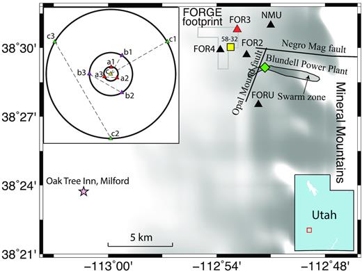
One broad-band SPAC array (FOR3, triangle) and one geophone SPAC array (OTI, star) nearby Milford, southwestern Utah. Station FOR3.UU a regional seismic station. The broad-band array is composed of one central station (FOR3), and three stations moved from the inner circle to the outer circle. Whereas array OTI is composed of ten geophone nodes. Inset, geometry of the two SPAC arrays.
The observed coherency functions from the two experiments are obtained using data recorded over a period of 9 hr. At both sites, the real and imaginary parts of the coherency curves are not in phase (Fig. S4), indicating that there are not directional noise sources nearby. However, for array OTI, sensors are stationary and record 9 hr of continuous data, while at FOR3, each array records for 3 hr. The coherency functions for array OTI are derived from raw data for each hour and the 9 hr of derived coherency functions are stacked to obtain the final coherency functions. For array FOR3, the coherency functions are directly derived from the 3-hr-long raw data. We evaluate the quality of the coherency function using the SD of the imaginary part. The SDs for all the distances at OTI are less than those at FOR3 except for the interstation spacing 17.3 m, at which the SDs of the imaginary part for the two SPAC experiments are almost the same. At OTI the imaginary part fluctuates around zero, while at FOR3 there are larger deviations from zero (Fig. S4; Table S4). Moreover, the coherency functions at OTI are much smoother and suffer from less localized noise spikes. The smoother function is most likely a consequence of stacking multiple windows. For an experiment with the same overall time duration, the resultant geophone coherency functions are better than those obtained from the broad-band array.
As seen in this example, the geophone sensors have great potential in SPAC applications compared to broad-band seismometers for the following reasons. First, the geophone SPAC experiments are easier to perform because the instrumentation is designed to be portable and easy to install. Secondly, even with the reduced bandwidth and sensitivity, frequencies greater than 0.1 Hz are well-recorded by the geophones. Ward & Lin (2017) used the same geophones to carry out a study to determine teleseismic receiver functions in a frequency band of 0.1–4 Hz. Ringler et al. (2018) in testing these instruments found that for frequencies greater than 0.1 Hz the limiting factor is site noise not the instrument response. Thirdly, as described above, because of the potential for longer duration recordings, the resultant SPAC coherency functions from the geophone arrays appear to have higher signal quality.
The Vs profile at FOR3, closer to the Mineral Mountains, is faster at shallower depth than that at OTI (Fig. 10). In this example, the starting Vs models at the two sites are constrained using MMSPAC (Asten 2006). The Vs30s at FOR3 and OTI are 406 ± 12 and 334 ± 13 m s–1, respectively. The results agree with Vs profiles determined for the Salt Lake Basin that indicate locations closer to mountains have higher Vs30 values (thinner unconsolidated sediments) and do not generate lower-frequency surface waves. This overall difference in velocity model may partially account for the poorer quality of the coherency functions at site FOR3 compared to site OTI.
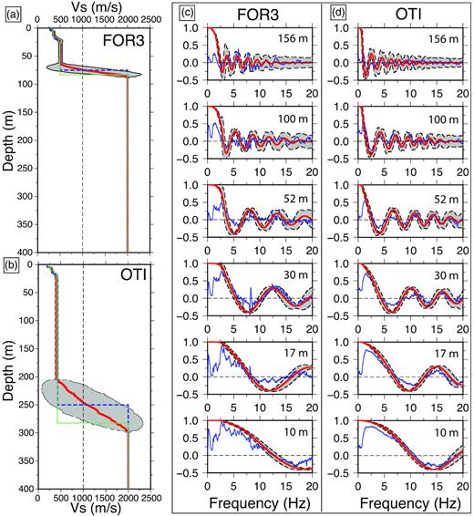
Vs models (red thick lines) with uncertainty areas characterized by |$1\sigma $| (grey area) for (a) FOR3 and (b) OTI. The starting model is indicated by the thin lines, while the Vs models estimated using MMSPAC are represented by the moderate dashed lines. Coherency function fits for sites (c) FOR3 and (d) OTI. The 2σ of the coherency functions are presented by grey areas. The thin lines are the observations, while the predicted coherency functions are indicated by the moderate lines.
6 DISCUSSION
The choice of model space has relatively small influence on success in obtaining a robust Vs structure using BMCI; this is supported by the following synthetic test. Given an appropriate model space, a series of models constructed using a Markov Chain can converge within a limited number of steps. The model space can be created in different ways. One way is to generate the model space around a known relatively accurate model; or when there is limited prior information, the model space can be defined using a wide range within the parameter space. For the models derived in this study, we started with a relatively well-constrained model space.
To test the potential limitations of BMCI when the model space is very large (wide range of Vs and layer thickness), we carried out a third synthetic test using a larger model space (Table S5) than that used in the first and second synthetics (|${m_0} \pm 0.2{m_0}$|, where |${m_0}$| is listed in Table S1). The resultant Vs profiles are within |$1\sigma $| uncertainty of the averaged Vs profiles derived from the BMCI for the three noise levels except for a layer within a depth range of 100–130 m (Fig. 11). Similar to the previous tests, the results for the synthetic coherency functions with 0 and 0.05 Gaussian white noise are almost identical, but are better than that derived from the noisiest synthetic data. The Vs profiles gradually and smoothly increase with depth, which is unlike the step increase of the given Vs profile. This is caused by the wide range of the model space and the nonlinear relationship between the model and the coherency functions, as well as by the velocity gradients, which could increase the uncertainties in interface depths.

Resultant Vs models for the third synthetic test with different noise levels: (a) 0.0, (b) 0.05 and (c) 0.2 using BMCI and a wider model space as listed in Table S5 and the same starting model to synthetic test 1. The average Vs profile is represented by the thick line, and the starting model is indicated by the moderate dashed line. The grey areas indicate |$1\sigma $| of the average Vs profiles.
The Vs30 of the given Vs profile (233 m s–1) is within the uncertainties of those estimated by BMCI in the wide-range model space. For tests without noise and with a noise level of 0.05, the Vs30s are 238 ± 28 and 238 ± 28 m s–1. respectively, which deviate less than 243 ± 31 m s–1 for the test with a noise level of 0.2. This indicates that the noise level in the data can affect the estimate of the Vs30. Compared to the two previous synthetic tests, the uncertainty areas of the Vs profiles are wider due to less convergence of models constructing the posterior Markov chain. However, the agreement of the Vs30s does suggest the feasibility of BMCI in the SPAC application to resolve the shallow structure of the earth even when little is known about the starting velocity structure.
Compared to the previous synthetic tests, the predicted average coherency functions have larger uncertainties (Figs 4, 12, S1a–S1b and S5). This means the resultant post-posterior models have more scatter. Moreover, the amplitudes of the average coherency functions at longer interstation spacing and higher frequency are smaller for all the tests with different noise levels, especially for the test without noise. Although having larger uncertainties, the average coherency functions derived from the wide-range model space fit the true ones well. Moreover, the frequencies at which the coherency functions cross zero are almost the same for the predicted and synthetic coherency functions. These agreements suggest the effectiveness of BMCI even if the model space is relatively unconstrained.
Coherency function fits for synthetic test 3 with a noise levels of 0.05; and those for noise levels of 0.0 and 0.2 are shown in Fig. S5. The red moderate lines indicate the average coherency functions from the posterior velocity models. The 2σ of the coherency functions are presented by grey areas behind moderate and thin lines. The blue thin lines are the summation of the coherency functions predicted by the true model in Fig. 3.
Compared to other SPAC approaches (Okada 2003; Asten 2006; Stephenson & Odum 2010), BMCI has the following advantages. First, the Bayesian inversion in the coherency domain provides mathematically rigorous uncertainties in the velocity model, which engineering and scientific communities will greatly appreciate. Secondly, BMCI resolved Vs models in an urban sedimentary basin that are very comparable to those from an earlier investigation using MMSPAC but with greater confidence in the final model uncertainties. Thirdly, we showed that BMCI is relatively insensitive to the initial model. Fourthly, BMCI works well even with noisy (lower coherency) microtremor array data.
The nearest neighborhood approach (NNA), another way to directly fit the SPAC coherency functions (Wathelet et al.2005), also randomly generates a number of models in a well-arranged model space like that in this study. The major difference between NNA and BMCI is that in the BMCI methodology a Markov Chain of models is formed and poorly fitting models are replaced by better models. This leads to a convergence of the solution and hence a tighter resultant model pool around the true model for BMCI relative to NNA.
Asten & Hayashi (2018) found that inclusion of poor coherencies in the inversions generates a bias to high Vs values. Thus, including poor coherencies at high or low frequencies in the data for BMCI might degrade the confidence in the BMCI. Asten (2006) suggested that the SD of the imaginary part of coherency can be used to represent the noise level when the wavefield is omnidirectional. This assumption is satisfied for all the urban SLV sites, and as shown in Fig. 8(a) and listed in Table S2, there is no clear correlation between the noise level and the Vs30 difference at these SLV sites. The SDs of the imaginary components are typically less than 0.1 (Fig. S4; Table S2). Moreover, the real and imaginary components of the coherency curves are not in phase (Fig. S2). Given the analysis of the imaginary component, there is little reason to suspect significant Vs bias in the BMCI results for the SLV data.
SPAC is often used to resolve the shallow Vs structure, while ambient noise tomography typically images Vs structure greater than 1 km (e.g. Wang et al.2017; Wu et al.2017). In this study, we found using BMCI in both synthetic tests and for sites with deep basin structure (e.g. FS, RIV and SJF) that Vs profiles down to 300–400 m are well resolved indicating the potential of BMCI to image the deeper Vs structure given high-quality SPAC functions. This is consistent with some previous SPAC studies that imaged depths greater than 400 m (e.g. Boore & Asten 2008; Okada 2003). Imaging greater depths with SPAC allows for the possibility to bridge the resolving depths between ambient noise tomography and the SPAC applications and thus provide a more complete picture of subsurface velocity structure.
Limiting factors for resolving depth with SPAC include array aperture, the bandwidth and sensitivity of the seismometers, and poor signal-to-noise represented in the coherency functions. For array aperture, the radius of the array approximates the maximum recoverable depth (Walthelet et al.2008). As discussed in Section 5, the geophones have good recording capabilities for frequencies greater than 0.1 Hz, and given the ease of deployment, these instruments can be deployed in large arrays for several hours to several days providing ample data for stacking to achieve high-quality coherency curves. Thus, based on our analyses and synthetic tests, a potential use for BMCI is to utilize SPAC together with optimized arrays to image to greater depths.
7 CONCLUSIONS
We develop a novel BMCI method for modelling near-surface Vs profiles using SPAC coherency functions. Importantly, we are able to provide quantitative uncertainties on the resultant models. This new method has been applied to data sets collected using both broad-band and geophone data with good results. An important finding of this study is that geophone data have sufficient bandwidth and sensitivity for use in SPAC analysis. The results obtained using the new method compare well to results obtained using MMSPAC for the same data, and resulting Vs30 values and depths of unconsolidated sediments determined for sites in the SLV compare well with the local community velocity model. We also showed using synthetics that the modelling is not dependent on the starting model and that average/smooth models can be determined even when little is known of the velocity structure (model space). Results from synthetic tests show that noise affects longer interstation spacings more than the smaller spacings, and the long duration data set collected using the geophone data showed the benefit of being able to stack longer time durations to improve signal quality. The resolution of the Vs profiles down to 300–400 m demonstrates the potential of BMCI in imaging deeper subsurface structure using SPAC. Additionally, geophones have no apparent limitation in SPAC applications when the frequencies of interest are higher than 0.1 Hz.
SUPPORTING INFORMATION
Figure S1a. Coherency function fits for the first synthetic test in an omnidirectional wavefield with distinct noise levels: (A) 0.0, (B) 0.05 and (C) 0.2. The red lines indicate the averages coherency functions from the posterior velocity models. 2σ of the coherency functions are presented by grey areas behind the red and blue lines, and the blue lines are the summation of the coherency functions predicted by the given model in Fig. 3 and the zero-mean Gaussian random variable with the standard deviations of 0.0, 0.05 and 0.2, respectively.
Figure S1b. Coherency function fits for the second synthetic test in an omnidirectional wavefield with distinct noise levels: (A) 0.0, (B) 0.05 and (C) 0.2. The red lines indicate the averages coherency functions from the posterior velocity models. 2σ of the coherency functions are presented by grey areas behind the red and blue lines, and the blue lines are the summation of the coherency functions predicted by the given model in Fig. 3 and the zero-mean Gaussian random variable with the standard deviations of 0.0, 0.05 and 0.2, respectively.
Figure S2a. Coherency functions for the sites CAM, FS, JRP, LP and RIC. The red lines indicate the real part of the coherency functions, and the blue lines indicate the imaginary part.
Figure S2b. Coherency functions for the sites BEN, MAG, RIV, ROS and SJF. The red lines indicate the real part of the coherency functions, and the blue lines indicate the imaginary part.
Figure S2c. Coherency functions for the sites SD, HER, FTT and VEC. The red lines indicate the real part of the coherency functions, and the blue lines indicate the imaginary part.
Figure S3a. Coherency function fits for the sites CAM, FS, JRP, LP and RIC. The red lines indicate the average coherency functions from the posterior velocity models. 2σ of the coherency functions are presented by grey areas behind the red and blue lines. The blue lines are the observations.
Figure S3b. Coherency function fits for the sites BEN, MAG, RIV, ROS and SJF. The red lines indicate the average coherency functions from the posterior velocity models. 2σ of the coherency functions are presented by grey areas behind the red and blue lines. The blue lines are the observations.
Figure S3c. Coherency function fits for the sites SD, HER, FTT and VEC. The red lines indicate the average coherency functions from the posterior velocity models. 2σ of the coherency functions are presented by grey areas behind the red and blue lines. The blue lines are the observations.
Figure S4. Comparison of coherency functions for the broad-band array FOR3 (left-hand panels) and the geophone array OTI (right-hand panels). The red lines indicate the real part of the coherency functions, and the blue lines indicate the imaginary part.
Figure S5. Coherency function fits for the third synthetic models with distinct noise levels: (A) 0.0, (B) 0.05 and (C) 0.2 as shown in Fig. 12. The red lines indicate the average coherency functions from the posterior velocity models. The 2σ of the coherency functions are presented by grey areas behind the red and blue lines as background. The blue lines are the summation of the coherency functions predicted by the starting model in Fig. 3 and the zero-mean Gaussian random variable with the standard deviations of 0.0, 0.05 and 0.2, respectively.
Table S1. True velocity model used for the first and second synthetic tests.
Table S2. SDs of the imaginary part of the coherency functions at six distances and the averages at the 14 SLV sites.
Table S3. Data durations and time windows to calculate SPAC functions for the 14 SLV broad-band sites, FOR3 (broad-band array), and OTI (geophone array). The status of stacking of the SPAC functions is also elaborated.
Table S4. Minimum and Maximum values of the imaginary part of the coherency functions at the broad-band array FOR3 and the nodal array OTI.
Table S5. Ranges of thicknesses and Vs for the third synthetic test.
Please note: Oxford University Press is not responsible for the content or functionality of any supporting materials supplied by the authors. Any queries (other than missing material) should be directed to the corresponding author for the paper.
ACKNOWLEDGEMENTS
The BMCI code is available upon request. We thank the editor, two anonymous reviewers, and Morgan Moschetti for their constructive comments, which greatly improve the manuscript. We gratefully thank Andy Trow, Stephen Potter and Zongshan Li for acquiring the SPAC data in Milford, southeast Utah. Most of the figures in this manuscript were plotted with Generic Mapping Tools (GMT, Wessel & Smith 1995). We thank Jack Odum and David Worley (both USGS) for their technical expertise in acquiring the Salt Lake Valley microtremor data. Funding for the Salt Lake Valley microtremor data was provided by the USGS Earthquake Hazards Program. This work (including collection of the Milford data) was partially supported by the U.S. Department of Energy, Office of Energy Efficiency and Renewable Energy's (EERE) Geothermal Technologies Office under Award Number DE-EE0007080. Additional funding was supplied the State of Utah. All data are available from William Stephenson via ScienceBase (https://doi.org/10.5066/P9OXYQST,). Any use of trade, product, or firm names is for descriptive purposes only and does not imply endorsement by the U.S. Government.
