


SUMMARY
In December, 2009, a rare sequence of earthquakes initiated within the weakly extended Western Rift of the East African Rift system in the Karonga province of northern Malawi, providing a unique opportunity to characterize active deformation associated with intrabasinal faults in an early-stage rift. We combine teleseismic and regional seismic recordings of the largest events, InSAR imagery of the primary sequence, and recordings of aftershocks from a temporary (4-month) local network of six seismometers to delineate the extent and geometry of faulting. The locations of ∼1900 aftershocks recorded between January and May 2010 are largely consistent with a west-dipping normal fault directly beneath Karonga as constrained by InSAR and CMT fault solutions. However, a substantial number of epicentres cluster in an east-dipping geometry in the central part of the study area, and additional west-dipping clusters can be discerned near the shore of Lake Malawi, particularly in the southern part of the study area. Given the extensive network of hanging wall faults mapped in the Karonga region on the surface and in seismic reflection images, the distribution of events is strongly suggestive of multiple faults interacting to produce the observed deformation, and the InSAR data permit this but do not require it. We propose that fault interaction contributed to the seismic moment release as a series of Mw 5-to-6 events instead of a normal main shock–aftershock sequence. We find the depth of fault slip during the main shocks constrained by InSAR peaks at less than 6 km, while the majority of recorded aftershocks are deeper than 6 km. This depth discrepancy appears to be robust and may be explained by fault interaction. Structural complexities associated with fault interaction may have limited the extent of coseismic slip during the main shocks, which increased stress deeper than the coseismic slip zone on the primary fault and synthetic faults to the east, causing the energetic aftershock series. There is no evidence of deformation at the Rungwe volcanic province ∼50 km north of the earthquake sequence between 2007 and 2010, consistent with previous interpretations of no significant magmatic contribution during the sequence.
1 INTRODUCTION
An unusual sequence of earthquakes occurred in December 2009 near the town of Karonga, Malawi. Only fourteen earthquakes with a magnitude >5 have occurred around the northern Lake Malawi rift between 1973 and 2017 (NEIC catalogue), and nine of those took place over a 2-week period between 6 and 19 December, 2009 (Fig. 1). More than 200 000 people were affected by these earthquakes, including four deaths and almost 200 injuries (Office of the United Nations Residence Coordinator 2009). Moreover, the sequence caused the evacuation of thousands of households for months, given the prolonged duration of the earthquake activity (Office of the United Nations Residence Coordinator 2009).
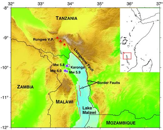
(a) Tectonic framework of the 2009 Karonga earthquakes on SRTM3 topography, with the Rungwe Volcanic Province shown as red triangles (Ebinger et al.1987, 1989), and red lines showing trace of primary border faults (Mortimer et al.2007; Accardo et al.2018). Stars show the locations of the largest earthquakes of the 2009 sequence from the NEIC catalogue; CMT locations for these events are shown in Fig. 2. White box indicates town of Karonga. (Inset) Red box shows study area in context of the East Africa rift system. Lake bathymetry is estimated from a surface fit to legacy MCS data (Lyons et al.2011).
The earthquakes are scientifically interesting for several reasons. First, the earthquakes did not occur on one of the >100-km-long border faults that bound the ∼50-km-wide sedimentary basins and elongate lakes (e.g. Lake Albert, Lake Tanganyika and Lake Malawi) of the Western Branch of the East African rift system (EARS, e.g. Ebinger et al.1991, 1999). The primary border fault in this segment of the EARS, the Livingstone Fault, is on the east side of the lake, 40–50 km northeast of the events, and thus the locations, mechanisms and event depths during 2009–2010 imply that the earthquakes are occurring due to slip on normal faults within the hanging wall (Fig. 1). As nearly all moderate-size earthquakes within the Western Rift of the EARS appear to be on major border faults (e.g. Jackson & Blenkinsop 1993; Nyblade & Langston 1995), the 2009 events offer a rare opportunity to evaluate how rifting is accommodated within the hanging wall of the system. A second unusual characteristic of this earthquake sequence is that in contrast to a classical main shock–aftershock sequence, the Karonga earthquake series comprises three large events with similar magnitudes of 5.8–6.0, with the largest event being the last one on 19 December 2009. Including two foreshocks, there were 14 other events with magnitudes in excess of 4.5, with all events in this primary sequence occurring in a 27-d period. Subsequent aftershock activity continued after 19 December 2009, but at a much lower magnitude level.
There are several possible explanations that can account for these earthquakes in the hanging wall and their seismological character: (1) a single immature fault in the hanging wall (e.g. Biggs et al.2010) with a heterogeneous distribution of stress and/or frictional properties (e.g. King & Nábělek 1985; Hillers et al.2007; Lohman & McGuire 2007; Hamiel et al.2012); (2) the interaction of multiple hanging wall faults with each other and/or with the border fault [for example, Hamiel et al. (2012) modelled the fault to have seven segments] or (3) a magmatic or fluid-driven swarm. The primary goal of this work is to determine which of these three models, or what combination of these three, is most plausible.
Numerical and analogue models suggest that once faults link to form favourably oriented, laterally continuous structures, they are capable of accommodating a large portion of deformation (e.g. Cowie et al.2000). For this reason, understanding the relative maturity of hanging-wall fault(s) associated with the Karonga earthquake is significant. Quantifying the maturity and behaviour of intrabasinal faults is also important for characterizing the accommodation of extension, either through distributed extension, or through hanging wall flexure.
Biggs et al. (2010) propose that the 2009 earthquakes occur on a single, immature, previously unmapped, west-dipping normal fault located near Karonga, which likely connects to a series of surface ruptures (Macheyeki et al.2015) identified by the Malawi Geological Survey as the St Mary’s Fault or St Mary Fault by Kolawole et al. (2018). The surface location of this structure, and its westward dip, are both well constrained by the surface deformation observed in the Interferometric Synthetic Aperture Radar (InSAR) analysis (Biggs et al.2010; Hamiel et al.2012). A single immature fault within the hanging wall could generate a sequence of events with similar magnitudes because it might have a more irregular large-scale geometry, such that ruptures are modulated by fault bends (e.g. King & Nábělek 1985). Furthermore, since young faults have accommodated less total slip, properties along the fault are likely to be more variable, including the presence of more asperities, which could discourage rupture of a large portion of the fault in a single event (e.g. Hillers et al.2007). Biggs et al. (2010) suggest that slip on a single fault can explain the pattern of surface deformation captured in InSAR data, but with slip during the final Mw 6.0 event occurring on a different portion of the fault than slip during the preceding events, which implies a rough, immature fault.
In the second model, a series of secondary faults within the hanging wall could interact with one another and/or the border fault to cause a sequence of events with similar magnitudes. Slip on one fault can cause loading and subsequent failure on another fault (e.g. Stein 1999). In the Karonga basin, this interaction could involve either a number of secondary faults or the border fault. Existing constraints on the geometry of secondary faults imply that fault interaction here could be important. Seismic reflection data collected in the lake to the east of the epicentral region image a series of closely spaced (∼5 km), west-dipping intrabasinal faults (Flannery & Rosendahl 1990; Mortimer et al.2007). West of the epicentral region, the east-dipping Karonga Fault has a clear topographic expression and appears to be one of the most prominent faults within the hinge zone of the flexing hanging wall (e.g. Laó-Dávila et al.2015). The close spacing and opposing dips of the Karonga and St Mary’s Faults implies that they intersect or otherwise interact at a fairly shallow depth within the crust (upper 10 km, e.g. Biggs et al.2010). Finally, pre-existing faults and basement fabrics have been recognized within the study area (e.g. the Precambrian Mughese Shear Zone) and may influence and interact with modern rift faults (e.g. Kolawole et al.2018). The possible participation of other fault structures in the deformation are not well determined from existing studies (e.g. any slip on segments beneath the lake will be invisible to InSAR).
For the third model, although there is no surface volcanism directly within the epicentral region, the potential role of deep magmatic fluids in the area is debated. There are hot springs in northern Malawi (Dulanya 2006), and the active Rungwe volcanic province is 50–70 km to the north (Fig. 1). Rungwe is the most southerly surface expression of volcanism in the EARS and one of a handful of volcanic provinces in the Western Rift, which is less magmatic than other parts of the EARS (e.g. Ebinger et al.1989). The only previous earthquake sequences in the southern EARS that exhibit similar swarm characteristics are demonstratively volcanic. These include eight events with Mw > 5 (the largest event occurring third in the sequence) associated with volcanic diking and subsequent eruption in northern Tanzania (e.g. Calais et al.2008; Fischer et al.2009), and three Mw 5.1–5.2 events over a 3-d period associated with a major eruption at Nyiragongo volcano eruption near Lake Kivu (Shuler & Ekström 2009). Previous InSAR results of the Karonga sequence (Biggs et al.2010; Hamiel et al.2012) imply that the majority of the moment release is on shallow tectonic faults, and there is no evidence for dyke or fluid involvement in the sequence. We have processed InSAR data over a larger spatial area including the Rungwe volcanic province to further constrain the potential for volcano–tectonic interactions during this earthquake sequence.
To distinguish between these models, we present an analysis of data recorded with a small network of seismometers deployed for four months following the earthquake swarm (January–May 2010) to characterize the spatial and temporal distribution of seismicity. Further, we compare these results with new models of the 2009 main shocks including ground deformation from InSAR and analysis of teleseismic and regional seismic waves. Our combined seismic and InSAR analysis in this paper will evaluate the three models for why the 2009 earthquakes near Karonga did not follow a normal main shock–aftershock sequence.
2 DATA AND METHODS
2.1 Local aftershock array
At the time of the 2009 earthquake sequence, the nearest seismometers (from AfricaArray, AA) were separated by several hundred kilometers and only one of these stations was working in Malawi, in Zomba over 600 km to the south. The Geological Survey of Malawi requested assistance in monitoring the ongoing sequence, and we were able to secure five instruments for rapid deployment, including three RAMP (Rapid Array Mobilization Program) instruments from IRIS (www.iris.edu) and two additional instruments from Cynthia Ebinger. The five instruments were rushed to the Karonga region and deployed for a four-month period between 6 January to 6 May 2010. Combined with a relocated AA station in Karonga, this network provides up to six stations within an approximately 20×50 km region surrounding Karonga (Fig. 2). The five portable stations are intermediate-period, three-component seismometers that recorded at 100 Hz, while the AA station is a broadband sensor that recorded at 20 Hz. Continuous seismic data are available under network code YI_2010 at the IRIS Data Management Center (Gaherty & Shillington 2010).
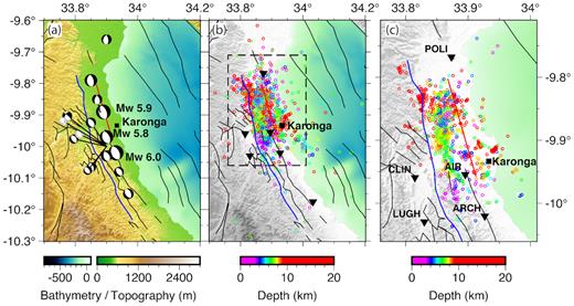
(a) CMT solutions for the 16 largest events that occurred in November–December 2009 (Table 2). Events are scaled by magnitude (Mw 4.5–6.0), with the largest three events labelled. Nine events from the Global CMT catalogue are plotted at their catalogue locations, with one shifted for clarity. The seven new solutions are indicated by the black lines pointing to the common centroid location used for these events; their relative locations are accurately represented as shown in Fig. S4. The two foreshocks are shown with grey mechanisms. Background topography relative to sea level is derived from the SRTM3 database, and lake bathymetry is estimated from a surface fit to legacy MCS data (Lyons et al.2011) relative to the lake surface (elevation ∼478 m). (b) Hypoinverse locations for approximately 1900 aftershocks recorded in Jan-May 2010 recorded using the local array (black triangles), with event symbol colours scaled by depth. Topography has been converted to grey scale for clarity. Black box shows zoom region of panel (c). (c) HypoDD relative relocations for ∼1050 events, coloured by depth. Note change in map scale relative to panels (a) and (b). For all panels, lines show mapped faults (Geological Survey of Malawi 1966; Mortimer et al.2007; Biggs et al.2010), with the Karonga (blue) and St Mary’s (red) Faults highlighted.
All collected seismic data were run through an automated detection and association algorithm to provide an initial set of possible events. Each event was visually inspected and P and S arrival times manually repicked by analysts. For all events with a minimum of four local stations providing traveltimes, the events were located using the hypoinverse location algorithm (Klein 2002) and several possible seismic velocity models. 1-D P-velocity models were derived for the Karonga region from a published model for an analogous portion of the southern EARS (Kim et al.2009), and preliminary analyses based on active-source and local earthquake data collected during the SEGMeNT experiment (Oliva et al.2016; Shillington et al.2016; Accardo et al.2018). We established Vp/Vs of 1.70 based on a trial-and-error analysis of residual behaviour. The resulting catalogues were evaluated based on overall mean and median traveltime residuals and estimated error ellipses, and the stability and number of events that had good solutions. The results shown in the figures are based on the preferred velocity model (dubbed SEG4), but some of the depth and statistical behaviour of the other models are presented in the results below. In general, the great bulk of the seismicity is located within the footprint of the six-station local array (Fig. 2b). Approximate local magnitudes (Ml) were determined using an automated estimate of displacement amplitudes in the direct P and S arrival windows. The preferred hypoinverse catalogue contains 1911 events with Ml ranging from −1 to 4.6, a mean RMS residual of 0.06 s, and a median location error (ellipse long axis) of 2 km.
Using this catalogue as a starting point, we performed double-difference relocation of the events using the hypoDD algorithm (Waldhauser & Ellsworth 2000) (Figs 2c, 3, Fig. S1). We utilized station-specific velocity models based on SEG4 with local correction for station elevation and sediment thickness. For events with <5 km separation difference, differential P and S times were calculated from the hand-picked traveltimes. We also incorporated cross-correlation differential times for event pairs with <3 km separation difference and correlation coefficient greater than 0.7. Requiring a minimum of eight constraints per pair, the resulting preferred differential-location catalogue contains 1049 linked events within a single cluster. We tested a variety of choices for data weighting and damping, and the final solution weighs the hand-picked and cross-correlation times approximately equally, and weighs the hand-picked S times half of the hand-picked P and cross-correlation times. The final locations produce RMS misfit of the hand-picked and cross-correlation differential times of 0.06 and 0.03 s, respectively.
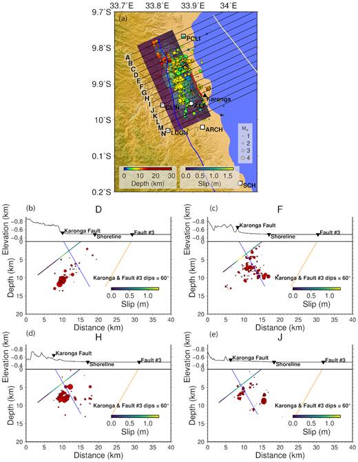
A map (subpanel a) and the four NE–SW cross sections D, F, H and J (subpanels b–e) showing inferred St Mary’s slip distribution (coloured by slip) and hypoDD aftershock locations during January–May 2010 (scaled by local magnitude), with offshore faults in yellow (Mortimer et al.2007), the Karonga Fault in blue (Geological Survey of Malawi 1966), and the surface rupture (in red) from the field survey conducted in October 2010 (Macheyeki et al.2015). Six local seismic stations are marked as white squares. All cross sections in (a) are shown in Fig S3.
The complete hypoinverse and hypoDD catalogues are available as direct downloads in the supplement.
2.2 Geodetic data
2.2.1 2009 earthquakes
We used InSAR data recorded by the Advanced Land Observation Satellite (ALOS-1) of the Japan Aerospace Exploration Agency and from multiple beams of the Envisat satellite of the European Space Agency spanning the earthquake sequence (Figs 4a–c and Fig. S2). We used the same data as Biggs et al. (2010), but we processed them independently, used a different slip inversion strategy, and considered the role of multiple faults. ALOS data are processed using using the ISCE software version 170806 (Rosen et al.2012) with topographic effects removed using the Shuttle Radar Topography Mission topography (Farr et al.2007), and all interferograms were unwrapped using SNAPHU (Chen & Zebker 2002). Envisat data are processed using the Caltech/JPL-developed software ROI_PAC (Rosen et al.2004) with the same procedure for topography removal and unwrapping, which can generate similar interferograms to the ISCE-derived products.
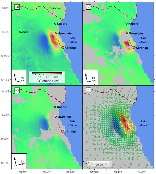
The unwrapped interferograms used in the fault slip inversions, and the stacked, downsampled measurements of LOS change. The black line in (a–c) indicates the locations of fault rupture from Macheyeki et al. (2015). (a) ALOS-1 between 23 September and 24 December, also showing the locations of major towns and the surface rupture (black line) from Macheyeki et al. (2015). Spacecraft heading shown as black arrow and LOS (with angle from vertical) shown as grey arrow. (b) Envisat between 1 December and 5 January. (c) Envisat between 6 September and 24 January. (d) Example of downsampled ALOS-1 interferogram (from a) using resolution-based quad-tree decomposition algorithm.
We processed one ALOS-1 pair and five Envisat pairs during the coseismic time span, but only the ALOS-1 interferogram and two Envisat interferograms, which remain coherent around the centre of surface deformation, were used for fault-slip inversion (Table 1). Three other coseismic interferograms from Envisat are not included as the input of inversion, but we compare them with the predictions of the forward model as an independent test (Fig. S2).
Interferograms used in this study. The first one is from ALOS PALSAR and the rest are from ENVISAT ASAR.
| No. | Dates (yymmdd) | Used in fault inversion | Beam number | Orbit | Baseline (m) | Figures |
|---|---|---|---|---|---|---|
| 1 | 090923-091224 | Yes | ALOS | Ascending | 100 | Fig. 4a |
| 2 | 091201-100105 | Yes | 3A | Ascending | 150 | Fig. 4b |
| 3 | 090906-100124 | Yes | 4A | Ascending | –70 | Fig. 4c |
| 4 | 090518-100118 | No | 2D | Descending | 20 | Fig. S2 |
| 5 | 091217-100121 | No | 2A | Ascending | 230 | Fig. S2 |
| 6 | 090531-091227 | No | 5D | Descending | –60 | Fig. S2 |
All three interferograms used in the inversion are downsampled using a resolution-based quad-tree decomposition algorithm (Lohman & Simons 2005) for achieving computational efficiency. A total of 1476 points (731 from the ALOS interferogram, 397 from the Envisat interferogram 3A and 348 from the Envisat interferogram 4A) are collected to reflect coseismic surface deformation (line-of-sight changes) as the input (Fig. 4d). To determine an estimate of fault location and geometry, we adopt the direct search algorithm that uses neighbourhood approximation in parameter space (Sambridge 1999), assuming a uniform fault dislocation and a homogeneous elastic half-space (Okada 1985). The initial model is set to the best-fitting fault geometry from Biggs et al. (2010). Once the optimal estimate of fault plane is found under these assumptions, we set up an automated fault model discretization with distributed slip on triangular dislocations (Barnhart & Lohman 2010) with a depth-dependent cell size that is based on checkerboard tests done by Hamiel et al. (2012). A linear growing factor is set up so that the size of a fault patch is 0.5 km when depth is less than 1.5 km and is 3 km when depth is 9 km, which is within resolution capabilities of models as seen from the checkerboard tests. We perform the inversion using all the input points of surface deformation and the estimated fault geometry, assuming a homogeneous elastic half-space (Fig. 5). We use second-order Tikhonov Regularization in our smoothing matrix and determine the weighting parameter using the |$_{j}\mathcal {R}_{i}$| approach, and evaluate the trade-off between smoothing and model fit using an L-curve (Barnhart & Lohman 2010).
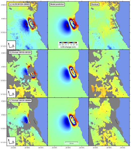
The data (left-hand column), model prediction (centre column), and residual after data minus model (right-hand column) for three interferograms that were unwrapped and then rewrapped using the same colour scale. (a) ALOS-1 between 23 September and 24 December, same as Fig. 4(a). (b) Envisat between 1 December and 5 January, same as Fig. 4(b). (c) Envisat between 6 September and 24 January, same as Fig. 4(c). The modelled interferograms are generated using the best-fitting single-fault slip distribution. The black line indicates the locations of fault rupture from Macheyeki et al. (2015).
We also compare the optimal fault geometry to mapped surface ruptures (Macheyeki et al.2015), existing fault locations (Geological Survey of Malawi 1966), and seismic profiles in Lake Malawi (Mortimer et al.2007). Motivated by these additional datasets as well as the aftershock relocations, we test alternative fault geometries based on these constraints, and perform inversions to assess how the slip distribution changes.
To determine the effects on the slip distribution caused by assuming a layered elastic model instead of a homogeneous half-space, we perform the distributed slip inversion using the preferred seismic velocity model SEG4 as a layered half-space (Fig. S3). While the homogeneous half-space model was calculated using triangular dislocations, for the layered half-space model, we use rectangular dislocations in the software EDGRN/EDCMP (Wang et al.2003). To convert from triangular to rectangular dislocations, we manually discretized the preferred fault plane into 248 rectangular patches, with the size similar to the best triangularly discretized fault model. Parameters for S-wave velocity and density in EDGRN are derived from SEG4 P-wave velocity, using the empirical relationships given by Castagna et al. (1985) and Quijada & Stewart (2007), respectively. We apply the same smoothing criteria to the slip inversion, and compare the results to the slip distribution from the homogeneous elastic half-space.
Since the aftershock hypocentres suggest the involvement of multiple faults (Fig. 3; see Section 3.1 for details), we also carry out slip inversions using multiple fault planes. The first fault plane is the optimal estimate from the uniform-slip search algorithm, and the geometry of the second fault plane is inferred from the east-dipping Karonga Fault or a west-dipping fault following an alignment/cluster of aftershocks. We manually discretize both faults with a cell size similar to the final discretization of the single fault inversion, and invert for distributed slip on triangular dislocations using the same algorithm from the single fault inversion. Once the slip distribution is calculated, we compare the fit with the results from the single fault inversion, and discuss if the addition of the second fault significantly alters or improves the model.
2.2.2 Time-series including Rungwe volcanic province
We used 150 ALOS-1 interferograms of various timespans to construct an InSAR time-series covering the 2007–2010 time period for the northern Lake Malawi/Rungwe Volcanic Province region using the method of Henderson & Pritchard (2013). We estimate the error on the time-series by quantifying the variance of the time-series in areas with no deformation. Based on analysis of pixels located in the north of our coverage area (far from the sources of deformation), scatter for the time-series is about ±2 cm, which is similar to error bounds from other ALOS-1 time-series (e.g. Chaussard et al.2013; Ebmeier et al.2013).
2.3 Focal mechanisms from telesismic and regional seismograms
The focal mechanisms of the largest earthquakes of the December 2009 sequence can be characterized using moment–tensor analysis. The global centroid-moment tensor (GCMT) catalogue (Ekström et al.2012) lists nine events in the period December 6–19 (Table 2), with the smallest event having Mw = 4.9 and the largest Mw = 6.0. We complement the GCMT catalogue by applying the standard GCMT analysis to several smaller events that were well recorded by stations of the Global Seismographic Network and AfricaArray (Nyblade 2007) at regional (up to |${\sim }30\, ^{\circ }{\rm }$|) epicentral distance (Table 2). We successfully modelled seven additional events that span the time window of 22 November through 19 December (Fig. 2a). These events include two foreshocks (events 1 and 2 in Table 2) to the first damaging event on December 6 (event 3). Due to the small size of these events, we were not able to simultaneously constrain their locations and moment–tensor solutions. We first utilized a relative relocation algorithm (Howe 2019) similar to that of Cleveland & Ammon (2013) and confirmed that the events fall in a tightly clustered region (Fig. S4). Based on this result, the hypocentres for the small events were fixed at a location of |$10\, ^{\circ }{\rm S}$|, |$33.9\, ^{\circ }{\rm S}$| and 12-km depth, and the fault-plane parameters were determined.
CMT analysis of primary event sequence. Events in global CMT catalogue (Ekström et al.2012) are marked with a “*”. All other events have fixed location. All events are from the year 2009.
| No | Mon. | Day | Hour | Min. | Sec. | Lat. | Lon. | Depth | Scalar | Mag | Mw | Strike | Dip | Rake |
|---|---|---|---|---|---|---|---|---|---|---|---|---|---|---|
| (km) | Moment (N-m) | (NEIC) | ||||||||||||
| 1 | 11 | 22 | 20 | 39 | 09.20 | −10.00 | 33.90 | 12 | 1.01E+16 | 4.6 | 4.6 | 145 | 43 | −105 |
| 2 | 11 | 25 | 21 | 14 | 33.50 | −10.00 | 33.90 | 12 | 8.39E+15 | 4.5 | 4.5 | 113 | 50 | −147 |
| 3* | 12 | 06 | 17 | 36 | 39.83 | −9.97 | 33.90 | 12 | 4.90E+17 | 5.8 | 5.7 | 162 | 36 | −81 |
| 4 | 12 | 06 | 17 | 58 | 15.40 | −10.00 | 33.90 | 12 | 4.18E+16 | 5.3 | 5.0 | 157 | 44 | −74 |
| 5* | 12 | 06 | 18 | 00 | 05.83 | −10.03 | 33.90 | 12 | 8.18E+16 | 5.3 | 5.2 | 165 | 43 | −75 |
| 6* | 12 | 06 | 18 | 29 | 17.85 | −10.15 | 33.97 | 14 | 6.48E+16 | 5.2 | 5.1 | 141 | 45 | −103 |
| 7 | 12 | 06 | 19 | 36 | 43.50 | −10.00 | 33.90 | 12 | 2.36E+16 | 5.1 | 4.8 | 162 | 36 | −87 |
| 8 | 12 | 07 | 03 | 35 | 43.80 | −10.00 | 33.90 | 12 | 1.51E+16 | 5.0 | 4.7 | 126 | 34 | −109 |
| 9* | 12 | 07 | 09 | 31 | 47.98 | −9.66 | 33.90 | 20 | 3.69E+16 | 5.0 | 5.0 | 202 | 35 | −62 |
| 10 | 12 | 07 | 18 | 09 | 40.30 | −10.00 | 33.90 | 12 | 2.43E+16 | 4.6 | 4.9 | 210 | 52 | −16 |
| 11* | 12 | 07 | 18 | 16 | 34.99 | −9.89 | 33.88 | 18 | 3.49E+16 | 4.9 | 5.0 | 202 | 49 | −54 |
| 12* | 12 | 08 | 03 | 09 | 01.44 | −9.89 | 33.89 | 12 | 1.01E+18 | 5.9 | 5.9 | 172 | 36 | −77 |
| 13* | 12 | 11 | 04 | 49 | 10.88 | −10.08 | 33.94 | 17 | 2.73E+16 | 5.0 | 4.9 | 149 | 49 | −84 |
| 14 | 12 | 11 | 20 | 06 | 28.40 | −10.00 | 33.90 | 12 | 1.85E+16 | 4.6 | 4.8 | 146 | 48 | −89 |
| 15* | 12 | 12 | 02 | 27 | 06.69 | −9.79 | 33.85 | 12 | 2.17E+17 | 5.5 | 5.5 | 182 | 37 | −75 |
| 16* | 12 | 19 | 23 | 19 | 20.43 | −10.02 | 33.93 | 12 | 1.09E+18 | 6.0 | 6.0 | 155 | 38 | −88 |
3 RESULTS
3.1 Aftershock sequence
The complete set of ∼1900 aftershock hypocentres forms a concentrated rectangular cloud trending NW–SE (Fig. 2b), coinciding with the bulk of the CMT locations, as well as the primary fault identified by Biggs et al. (2010). The spatial distribution of earthquakes terminates abruptly to the west, with very few events located west of the local array. A larger number of events are located beneath Lake Malawi to the east of the array, including a fairly concentrated cluster just southeast of Karonga town that forms part of a quasi-linear band paralleling the dominant cloud onshore. Hypocentral depths range from the surface to over 15 km depth, with the deepest events clustered in the far northwest region, as well as in the southeast corner directly beneath Karonga.
The more precise relative locations of the ∼1050 hypoDD events illuminate more features within the cloud of the seismicity than seen in the complete catalogue, providing greater clarity on likely fault activity (Fig. 2c). Overall, the spatial distribution of the events is similar to the absolute locations, with earthquakes clustered in the region of faulting inferred by Biggs et al. (2010), with a sharp boundary to the west, and several events distributed to the east. The faulting is further illuminated by plotting hypocentres in cross-section perpendicular to the strike of the St Mary’s Fault (Figs 3b–e and Fig. S1).
In the north, the events cluster in a confined, west-dipping body at 6–13 km depth that projects back to the surface location of the St Mary’s Fault (Fig. 3b). Stepping south into the middle of the cluster (Fig. 3c), the events shallow to <10 km depth, and appear to bifurcate into two trends: one dipping to the west from 2 to 10 km depth with a surface projection at the location of the St Mary’s Fault; and one dipping to the east from ∼5 to 10 km depth that may represent a deep extension of the Karonga Fault. This interpretation implies that the Karonga and St Mary’s Faults intersect near 5 to 8 km depth. Continuing south (Fig. 3d), the west-dipping St Mary’s Fault persists, while the east-dipping feature is no longer apparent in the aftershock patterns. Finally, in the southern portion of the sequence near Karonga village (Fig. 3e), the seismicity breaks into two to three subparallel west-dipping features indicative of synthetic faults with approximately 5-km spacing. One of the lineations at 2 to 10 km depth is consistent with St Mary’s Fault, suggesting that this fault is active over the entire length of the aftershock sequence. The additional features are active at larger depth (6 to 12 km), and they suggest west-dipping faults that would project to the surface beneath Lake Malawi.
There is a significant proportion of the aftershocks lying at or below the downdip limit of the primary slip surface inferred from InSAR analysis (<6 km; Fig. 6). While many of the aftershock lineations described above extend upward to depths <5 km, the mean depths of the catalogues are 7.1 and 7.5 km for the complete and hypoDD catalogues, respectively. The densest clusters of events in the hypoDD catalogue locate to the 5-10 km depth range. In addition, the approximate dips of the west-dipping lineations inferred from the cross-sections (Fig. 3) is of order ∼60°, steeper than the west-dipping focal planes inferred for the CMT events (generally 35–50°). Absolute depths are quite difficult to constrain using a limited distribution of stations directly above the events, as is the case here. Tests with alternative velocity models suggest that the spatial patterns interpreted above are robust, but the absolute depths can differ by an average of up to 2 km. Even with this uncertainty, most of the aftershocks still occur at greater depths than the primary slip zone inferred from InSAR.
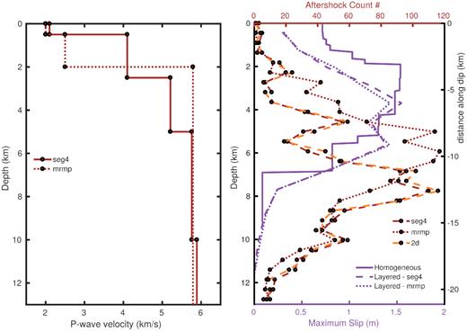
Left-hand panel: two P-wave velocity models tested for aftershock locations (MRMP and SEG4). Right-hand panel: histogram of fault slip (purple lines) from our inversions in homogeneous half-space and layered models compared to the distribution of hypoDD relocated aftershock depths using the two 1-D seismic velocity models (red lines), and a 2-D model approximation using station-specific sediment thickness (orange line). All models suggest that most geodetic coseismic slip is shallower than the majority of aftershocks.
The temporal and magnitude statistics of the complete hypoinverse catalogue are broadly consistent with a main shock–aftershock sequences on shallow crustal faults. Above a magnitude of completeness of 0.8, the sequence has a Gutenburg–Richter b-value of ∼0.8, and a modified Omori’s law decay exponent of 0.73. These parameters represent the aftershock behaviour in the time window of the local deployment, which begins approximately 18 d after the main shock, which we assume to be the largest event (19 December) of the primary sequence. As such, it does not describe the full complexity of the extended 27-d primary sequence, nor does it include the likely energetic 18-d period following the Mw 6 event (for which we have no events). To the extent that these statistics are representative, they imply a relatively energetic, slowly decaying aftershock sequence, with an anomalously low b-value (deficit of smaller events) relative to most normal-faulting sequences (Schorlemmer et al.2005). Low b-values are suggestive of high differential stress (Scholz 2015). Such a stress state is atypical of extensional systems, although similarly low b-values have been observed in other regions of the western rift (Lavayssiere et al. 2019). One interpretation is that the relatively high stress state suggests that the faults are relatively immature and occur in strong, intact crust, consistent with inferences from previous studies (Biggs et al.2010; Fagereng 2013).
3.2 Focal mechanisms
In map view, the CMT events fall along a NW–SE lineation (Fig. 2) that correlates well with the strike of the primary fault inferred by Biggs et al. (2010). Uncertainties in global velocity models result in absolute CMT locations determined to within only 10–20 km, and the north–south distribution of epicentres and precise correlation of the largest events with the region of highest slip is difficult to ascertain. The relative relocation analysis (Fig. S4) suggests that all of the events are tightly clustered within a ∼20-km-long linear trend, roughly consistent with the length of the primary faulting inferred from InSAR. The final, largest event in the sequence lies at the southern end of the cluster, which also agrees with the InSAR modelling (Biggs et al.2010).
The combined observed seismic moment for the 16 events (Table 2) is equal to 3.19 x 10¹⁸ N m, corresponding to a moment magnitude of Mw = 6.3. Most focal mechanisms suggest normal faulting on NW–SE striking fault(s), while two (including one foreshock) show evidence of a significant strike-slip component (events 2, 10). All events have moderate fault dips of 34–56°, depending on choice of fault plane. For most events, the west-dipping plane has a shallower dip. The two mechanisms with a strike-slip component fall at the northern end of the event cluster (Fig. S4). For one of these (event 10) there are sufficient data to carefully evaluate the robustness of the mechanism, and it is clear that the strike-slip component of this event is required.
For all events, depths appear to be shallow: most have a fixed GCMT value of 12 km, although four events give best solutions with depths of 14–20 km. For the largest events in the 2009 sequence, Biggs et al. (2010) determined shallow (<8 km) depths using teleseismic P waveform modelling.
3.3 InSAR slip distribution of the 2009 earthquake sequence
The best-fitting fault geometry from the uniform-slip inversion agrees with the locations of St Mary’s Fault and the surface rupture from the 2009 earthquakes, and dips at 38–45° to the west (Fig. S5); this result agrees with previous analysis of Biggs et al. (2010). The result indicates a fault plane that is 16.8 km long and 5.8 km wide, with an average slip amount of ∼0.83 m. The geodetic moment corresponds to a moment magnitude of Mw 6.2 similar to that found in previous work (3.22–3.5 × 10¹⁸ N m, Biggs et al.2010; Hamiel et al.2012) and close to the total seismic moment of 3.2 × 10¹⁸ N m (Mw 6.3) for the sequence. Since the result is not sensitive to the variation of rake between –70° and –110°, we select a rake of –90° assuming a pure normal faulting event. We utilized a dip of 38°, which is suggested by GCMT and Biggs et al. (2010), as the final dip value being used in the distributed slip inversion. The complete parameters used in the distributed slip inversion are listed in Table 3.
The best-fitting fault geometry used in the inversion of slip distribution.
| Parameter | Value | Comments |
|---|---|---|
| Strike | 156° | Constrained by the uniform slip inversion and surface rupture |
| Dip | 38° | From gCMT and Biggs et al. (2010) |
| Rake | -90° | Assuming a pure normal fault (e.g. Biggs et al.2010) |
| Depth of the Fault Top | 0 km | Constrained by surface rupture |
| Width | 15 km | Uniform slip inversion suggests at least 12 km |
| Length | 29 km | Uniform slip inversion suggests at least 17 km |
| Fault northern end | (33.84190°E, 9.75042°S) | From uniform slip inversion |
| Fault southern end | (33.95012°E, 9.98973°S) | From uniform slip inversion |
The result from the distributed slip inversion shows that the slip zone projects to a location at depth between the surface traces of St Mary’s Fault and Karonga Fault, where most aftershocks are located (Fig. 3a). The maximum slip is between 1.4 and 1.6 m depending on the smoothing level (Fig. S6), but always occurred at 2–5 km depth (Figs 3b–e and 6). The RMS misfit is 0.014 m (R2 = 0.95), similar to the expected data noise suggesting a very good fit to the geodetic observations at the determined smoothing level. The model resolution has been assessed in Hamiel et al. (2012) using a checkerboard test and we use the same subfault siz–depth relationship for each fault patch. The inversion result from the layered velocity model shows a similar slip distribution as a function of depth as the homogeneous half-space (Fig. 6), suggesting that the geodetic observations are robustly in favour of much shallower fault movement (<6 km) than the nominal GCMT centroid depths (12–20 km). This agrees well with the depth of the largest hypocentres (<8 km) determined using teleseismic P waveforms (Biggs et al.2010), and it is slightly shallower than the mean depth of the aftershock distribution (∼7 km).
We select two cases from the slip inversions using multiple fault planes to illustrate the impact of multiple faults. The first fault in both case is the St Mary’s Fault plane. The second fault of the first case shares the same geometry (strike, dip, location and dimension) as the optimal fault plane, but is 4.5 km deeper. In the second case, the second fault resembles the geometry of the east-dipping Karonga Fault with a dip of 60°. All the cells of the second faults also follow the same depth–size relationship which applies to the St Mary’s Fault plane. The results (Figs 8b, c, e and f) show that the models are similar in terms of both slip distribution and fit to the data (not shown). We do not think it is possible to argue that one model fits all of the data better than another given the poor interferogram quality—there are problems with coherence in the Envisat data and with the small number of interferograms overall, it is difficult to reduce the atmospheric noise. In both cases, slip along the second fault is confined within a small region, with a maximum slip of only ∼0.4 m. The primary optimal fault plane still accounts for over 90 per cent of the seismic moment, thus it is not likely that deeper west-dipping fault(s) or the Karonga Fault accommodated significant slip in the 2009 November–December earthquakes.
3.4 Regional InSAR time-series
The ALOS-1 time-series between 2007 and 2010 (Fig. 7) shows no significant deformation (±2 cm) at volcanoes in the Rungwe volcanic province. No deformation associated with the Karonga earthquake sequence was observed within the volcanic province. Individual interferograms suggest the presence of a seasonal signal (amplitude of 9 cm) in the northern part of the region (the signal is also apparent in the L2 residual plot for the time-series). The pattern shows maximum uplift in February–June and subsidence during the remaining months of the year. This uplift lags the typical rainy season (December–March) by approximately two months, and the correlation between the deformation and the wet/dry seasons suggests that the signal may be groundwater response. Surface deformation from the 2009 to 2010 Karonga earthquake sequence is clearly visible in the InSAR timeseries. The deformation pattern is located just north of the main cluster of located earthquakes and shows +15 cm and −10 cm motion in radar line-of-sight coordinates. Although not overly noticeable in the time-series (Fig. 7), postseismic deformation is evident in individual interferograms (Hamiel et al.2012).
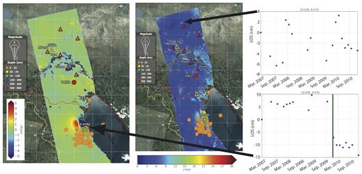
ALOS-1 time-series of InSAR phase change between 2007 and 2010. (a) Best-fitting linear ALOS time-series. Note that the numerical estimate for the linear rate very close to the earthquake location is not reliable. (b) L2 residual plot from the time-series show locations not fit well by a linear rate. For a and b: Red triangles are volcanoes, yellow are campaign GPS, labelled red, green and orange dots are cGPS, unlabelled orange circles are earthquakes during 2009-2010. No GPS stations were close enough to measure the ground deformation from the 2009 to 2010 sequence. (c) Seasonal signal in a rural part of Tanzania. Subsidence in June–Dec., uplift in February–May. (d) Deformation during the 2009–2010 earthquake sequence. Post-seismic deformation is clearer in individual interferograms (e.g. Hamiel et al.2012).
4 DISCUSSION
4.1 Were multiple faults involved in the earthquake sequence?
Based on the relocated aftershock distribution, it is clear that more than a single fault was involved in producing aftershocks between January and May 2010. The January and May 2010 sequence shows an east–west distribution spanning 30 km (Fig. 3). It appears to involve multiple west-dipping faults including the St Mary’s Fault, as well as a possible east-dipping deep extension of the Karonga Fault (Figs 3c–e and Fig. S1). The evidence for multiple faults is particularly compelling just west of the lakeshore between 9.90°S and 9.95°S, where there are several deeper clusters (>5 km depth) east of the trace of the St Mary’s Fault (Figs 2c and 3e). These events are well recorded by the local array, and are consistent with plausible west-dipping faults that breach the surface beneath Lake Malawi (Mortimer et al.2007), and are clearly inconsistent with the fault plane associated with the St Mary’s Fault. Coulomb stress calculations suggest that faults of this orientation and location (deeper and to the east of the primary slip zone) would be pushed closer to failure by slip on a St Mary’s type feature (Fagereng 2013).
The activation of an east-dipping fault beneath the centre of the sequence is less clear. This region is the most energetic portion of the sequence (in terms of number of events), and the events remain somewhat cloud-like, even following relocation with hypoDD. A planar east-dipping feature can be discerned in some of the cross sections (e.g. Fig. 3c), and the coincidence of this feature with a projection of the Karonga Fault provides a reasonable interpretation. However, a simple analysis of Coulomb stress change on the Karonga Fault due to the coseismic slip on the St Mary’s Fault (similar to Fagereng 2013) suggests a decrease of stress along Karonga Fault. Nevertheless, it is possible that the stress heterogeneity introduced by the fault intersection contributes to the large number of events, as well as the cloud-like seismicity pattern (e.g. Sumy et al.2013). Aftershock activation on intersecting antithetic faults have been observed in other extensional settings (e.g. Karasözen et al.2018; Lavecchia et al.2018; Walters et al.2018).
Whether multiple faults were involved during the November–December 2009 main shocks is harder to address. The InSAR data are permissive of multiple faults being active during the November–December 2009 sequence (Figs 8a–f), but we agree with Biggs et al. (2010) that the majority of slip occurred on the west-dipping St Mary’s Fault. Little slip is preferred on the alternate fault geometries suggested by the aftershocks, and the slip inferred from the InSAR data matches the total seismic moment of the November–December sequence quite well as found in previous work (Biggs et al.2010; Hamiel et al.2012). These results suggest that primary slip on the immature St Mary’s Fault excited subsequent slip on synthetic west-dipping hanging-wall faults beneath Lake Malawi and possibly on the east-dipping Karonga Fault.
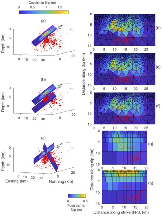
The inverted slip distributions during the 2009 earthquakes, and the comparison between different models in terms of their slip patterns. (a) Slip distribution using the best-fitting fault geometry (St Mary’s Fault) only. Purple line sketches the fault extent used by Hamiel et al. (2012). The shoreline of Lake Malawi is a black line, and aftershocks during January–May 2010 (using the velocity model seg4) are shown as red dots. (b) Slip distribution using the best-fitting fault geometry and another deep west-dipping fault, which shares the same strike and dip with the best-fitting fault. (c) Slip distribution using the best-fitting fault geometry and an east-dipping fault approximating the Karonga Fault. (d) Slip distributions using only the best-fitting fault geometry. (e) Slip on the St Mary’s Fault, using the two-fault model from (b). (f) Slip on the St Mary’s fault, using the two-fault model from (c). (g) Coseismic slip on the St Mary’s fault from Hamiel et al. (2012). (h) Postseismic slip on the St Mary’s fault from Hamiel et al. (2012). Note that (h) is plotted using a different colour scale. (d)-(h) are viewed at an angle normal to the fault plane.
The teleseismic and regional locations of the November–December 2009 events are also generally consistent with the sequence primarily being located on the St Mary’s Fault. While the absolute locations of the largest events in the sequence (events 3, 12, 15 and 16) that dominate the moment release are located systematically south of the geodetically inferred slip patch, the offset (∼5–10 km) is within that expected for location error for earthquake catalogues in Africa (e.g. Weinstein et al.2017) and globally (e.g. Weston et al.2014). The relative locations of these events follow a NW–SE trend parallel to the St Mary’s Fault, with a north–south extent that is quite similar to the length of the St Mary’s Fault in the geodetic models. Furthermore, the largest event in the sequence is to the south, consistent with InSAR modelling of this event (Biggs et al.2010). The events with a significant strike-slip component suggest activity on additional fault(s) in the northern portion of the sequence, perhaps associated with a change of basement crustal fabric inferred from potential field data (Kolawole et al.2018).
In summary, although the majority of slip and seismic moment release appear to be associated with the St Mary’s Fault, our results suggest that part of the main December earthquake series and the resulting aftershock series occurred on multiple interacting faults. These fault interactions may have contributed to the complexity of the Karonga earthquake series.
4.2 Depth of coseismic slip and aftershocks
We find that there is an offset in depth between the projected location of coseismic slip on the St Mary’s Fault and the distribution of aftershocks (Figs 3b–e and 8). This may be due in part to uncertainty in fault-plane geometry and/or event depths, but tests of both variations in fault dip and velocity models suggest that these uncertainties cannot explain the difference (Fig. 6 and Fig. S3). The InSAR observations prefer shallow slip (<6 km depth) on a fault dipping between 38° and 45°, shallower than the dip suggested by the aftershocks (∼60°). As discussed above, the absolute depth and apparent dip of the aftershock distribution could be shallowed by alternative velocity models, but it is clear that even in this case the bulk of the seismicity is deeper than 5 km, deeper than the peak slip (Fig. 6). Such a difference between the location of coseismic slip and subsequent aftershocks has been seen in a number of tectonic settings (e.g. Nissen et al.2010; Roustaei et al.2010; Elliott et al.2011; Wei et al.2015; Karasözen et al.2016, 2018; Lavecchia et al.2018). It is often interpreted as resulting from fault complexity that results in the arrest of coseismic slip, either due to changes in fault geometry (e.g. Elliott et al.2011; Karasözen et al.2018; Lavecchia et al.2018) or changes in fault strength and/or rate-state behaviour (e.g. Semmane et al.2005; Roustaei et al.2010; Wei et al.2015).
The total geodetic moment is similar to the total seismic moment as well as previous geodetic estimates (Biggs et al.2010; Hamiel et al.2012), so there is no geodetic evidence for the involvement of aseismic slip or fluids in driving the earthquake sequence, including fluids associated with the Rungwe volcanic province. Postseismic deformation is most likely caused by fault afterslip and not poroelastic relaxation or fault healing (Hamiel et al.2012). Afterslip is shallow (upper 2 km) and of relatively low magnitude, with a maximum slip of 40 cm compared to 120 cm of coseismic slip and a total moment between December 2009 and August 2010 that is about 40 per cent of the coseismic moment (Figs 8g and h, Hamiel et al.2012). The afterslip does not appear to have been important in producing aftershocks in the 2010 January–May period regardless of whether they are associated with St Mary’s fault or other nearby west-dipping faults, since few of our detected events occur in the upper 2 km (Figs 3 and 8). Further, we do not detect any continued deformation near the 2009–2010 afterslip location between 2014 and 2017 with Sentinel-1 InSAR analysis (Henderson et al.2017).
4.3 Regional and global comparison
The suggestion of intersecting faults in the 2010 aftershock data provides further context for understanding the sequence of main events in December 2009. With several Mw 5+ events that do not follow typical main shock–aftershock behaviour, the 2009 events suggest some basic characteristics of an earthquake swarm (Holtkamp & Brudzinski 2011), although there is insufficient local station coverage during the December 2009 period to adequately assess whether the events are truly swarm-like. Swarms are often associated with aseismic deformation and/or fluid migration (e.g. Holtkamp & Brudzinski 2011), neither of which is inferred here. In addition, the catalogue presented here suggests that by January 2010, the process can be characterized as an energetic aftershock sequence with magnitude and decay characteristics within the range of normal earthquakes. Rather than a swarm, Biggs et al. (2010) characterize the 2009 events as a sequence of moderate events, which they interpret as resulting from structural complexity on an immature St Mary’s Fault. We concur with the characterization as a sequence, but suggest that fault intersection and interaction also contribute to the complexity of the sequence.
While most of the cumulative slip during the main shock sequence appears to have occurred on the St Mary’s Fault, other nearby structures could have modulated failure on the St Mary’s Fault and explain the complexity of the sequence. An intersecting structure can form a geometrical barrier to fault propagation (e.g. King 1986), and the presence of such barriers could contribute to the occurrence of a complex series of events rather than one larger event (e.g. Elliott et al.2011; Karasözen et al.2016; Lavecchia et al.2018; Walters et al.2018). The intersection of the Karonga Fault with the St Mary’s Fault helps explain the depth distribution of the aftershock sequence described above, and it may also explain the along-strike complexity of the main December sequence. Variation in the interaction between these faults along strike could produce barriers that limit slip in any individual event. Additionally, magnetic data and geologic mapping constrain the tectonic grain in the Proterozoic basement in the region of the Karonga sequence (Kolawole et al.2018). A change in the orientation of this fabric is observed near Karonga town; it is oriented WNW to the north and NW to the south. The intersection of these ancient structures with the St Mary’s Fault may also contribute to the complex earthquake series, as suggested by Kolawole et al. (2018).
5 CONCLUSIONS
We combine teleseismic and regional seismic recordings, InSAR imagery, and recordings of aftershocks from a temporary (4-month) local network of six seismometers to examine the unusual 2009 Karonga earthquake series in the weakly extended Malawi Rift. Consistent with previous studies (e.g. Biggs et al.2010; Hamiel et al.2012), new analysis of InSAR data and global/regional CMT solutions from this study suggest that a west-dipping fault (the St Mary’s Fault) in the hanging wall is responsible for the majority of slip during the main shocks. However, aftershocks also delineate several other closely spaced west-dipping faults to the east of the St Mary’s Fault in the southern part of the study area and one possible east-dipping fault to the west in the central part of the study area; the latter appears to project to the surface trace of the Karonga Fault. These results suggest that the interactions of closed spaced and sometimes intersecting faults may have contributed to the complexity of the December 2009 Karonga earthquake series. InSAR data permit the involvement of multiple faults, but do not require it—we have modelled up to two, but the seismicity suggests that more may have been active. However, the clear majority of coseismic slip occurred on the St Mary’s Fault in agreement with previous work (Biggs et al.2010; Hamiel et al.2012). We suggest that structural complexities on the St Mary’s Fault resulting from the intersection of the St Mary’s with other faults at depth may have limited coseismic slip during the main shocks to shallow depths. Structural heterogeneity on the St Mary’s Fault caused by its youthfulness (Biggs et al.2010) and the interaction of multiple faults at depth may also explain the occurrence of a series of similar sized earthquakes instead of a normal main shock–aftershock series during the first month of activity.
The majority of aftershocks occur at greater depths (>6 km) than the slip during main shocks based on InSAR data (<6 km); this depth discrepancy appears to be robust. We suggest that shallow rupture during the December 2009 main shock series increased stress on deeper faults and nearby favourably oriented faults (e.g. Fagereng 2013), causing the energetic aftershock series. The aftershock series is associated with unusually low b-values for extensional faults (Schorlemmer et al.2005), which indicates high differential stress (Scholz 2015), consistent with rupture on immature faults in strong crust (e.g. Biggs et al.2010; Fagereng 2013).
We calculated InSAR interferograms over a broader area than previous studies, and do not observe evidence for ground deformation from fluids/magma or aseismic slip near Karonga or the Rungwe Volcanic Province.
SUPPORTING INFORMATION
karonga2010_hypo2k.loc.tex. ASCII text file containing complete Hypoinverse aftershock catalogue.
karonga2010_hypoDDv2.loc.tex. ASCII text file containing hypoDD aftershock catalogue.
Figure S1. The complete 14 E–W cross sections from Fig. 3 a covering the faulting region, each labelled A to N. See Fig. 3 caption for further details of the symbols and colours.
Figure S2. Envisat interferograms that were too noisy to use in the inversion and the predicted interferograms generated from the preferred slip distribution using the three interferograms in Fig. 5 as described in the main text. The modelled surface deformation is wrapped using a radar wavelength of 5.6 cm (the wavelength of Envisat ASAR sensor).
Figure S3. Top panel: modelled slip distribution using the layered velocity model seg4 and surface deformation from the three interferograms used in the half-space inversion (Fig. 5). The fault is discretized into 248 rectangular cells with a varying size, resembling the size of cells used in the half-space inversion (Fig. 8). Bottom panel: shows the ALOS-1 data (left, Figs 4a and 5a), modelled interferogram (centre) and residual for the resampled data.
Figure S4. Surface-wave relative location analysis (Howe 2019) applied to CMT events from Table 2 in manuscript. (A) Initial PDE locations (white squares) and final relative event locations (red circles). Location of the cluster centroid is not constrained by the analysis. (B) Relative-location error ellipses for each event. Errors are generally <2 km and NW–SE trend is robust. (C) Final CMT mechanisms plotted at accurate relative locations. Entire cluster has been shifted ∼15 km north and ∼3 km east to correspond to the dominant faulting inferred from InSAR analysis. Event(s) with strike-slip component discussed in the text are located at the northern end of the cluster.
Figure S5. The relationship between the model InSAR RMS misfit and the dip of the fault plane used in the model, when other fault parameters remain fixed. We select dip = 38° (doubled circle) as our preferred fault plane and describe the model results in the main manuscript.
Figure S6. L-curve showing InSAR coseismic slip model roughness versus model minus data difference) and corresponding slip distributions at different points along the L-curve. We select the results from the third row as our preferred, best-fitting model in the main text.
Please note: Oxford University Press is not responsible for the content or functionality of any supporting materials supplied by the authors. Any queries (other than missing material) should be directed to the corresponding author for the paper.
ACKNOWLEDGEMENTS
This project was funded by the U.S. National Science Foundation OCE-1049620 (to J.B.G., D.J.S., S.L.N. and M.E.P.) and EAR-1109512 (to M.E.P.). Funding for seismometer deployment was provided by Lamont-Doherty Earth Observatory, the Earth Institute at Columbia University, and the Incorporated Research Institutions for Seismology (IRIS) Portable Array Seismic Studies of the Continental Lithosphere (PASSCAL) Rapid Array Mobilization Program (RAMP). We thank Cynthia Ebinger and the University of Rochester for the loan of 2 seismometers used in the deployment. W.Z. acknowledges the support from the Overseas Ph.D. Scholarship granted by the Ministry of Education, Taiwan. We acknowledge Andreas Mavrommatis for starting the InSAR analysis as a senior thesis project at Cornell University that was funded by the Engineering Learning Initiatives program and Joey Durkin for help with InSAR processing. ALOS-1 InSAR data were provided by the Japanese Aerospace Exploration Agency through the Alaska Satellite Facility. Envisat InSAR data were provided by the European Space Agency. Statistical seismology software was obtained from the website maintained by Zhigang Peng and Brendan Sullivan at Georgia Institute of Technology. We gratefully acknowledge assistance from Leonard Kalindekafe, Winstone Kapanje, and Charles Kankuzi and from the Malawi Geological Survey Department. We thank the two anonymous reviewers, Assistant Editor and Editor for comments that improved the manuscript.
