


SUMMARY
Anisotropy of magnetic susceptibility (AMS) measurements, a commonly used method, has been applied in loess to determine the dominant palaeowind direction during the Pleistocene. During the last session of sampling and detailed magnetic investigation of the Early Middle Pleistocene loess/palaeosol succession at Paks (Hungary), ‘irregular’ (i.e. non-flow-aligned) magnetic fabrics (MFs) were revealed from sedimentary records having uniform sedimentary parameters. Knowledge about the origin of irregular loess fabrics is still limited, although they may carry additional palaeoenvironmental information. The appearance of irregular MF suggests that a constant set of palaeoclimatological conditions, as indicated by the layer characteristics, was interrupted by abrupt events. To characterize the unusual event horizons, the MF of the horizons and those of both the under- and overlying material were analysed and compared by rock magnetic methods, such as hysteresis, temperature dependence of magnetic susceptibility, and AMS.
The analysis separated three types of irregular fabrics and revealed three scenarios that might have been responsible for the forming of the irregular MF: abrupt climate changes, including rapid (catastrophic) weather events (e.g. intensification of strong wind- or water-lain processes); short-term pedogenesis during glacials; and post-depositional deformation triggered by mass movements or seismic activity.
1 INTRODUCTION—THE MAGNETIC FABRIC OF LOESS
In the course of the detailed sampling and magnetic fabric (MF) investigation of the Paks loess profile (Hungary; Bradák et al.2018a,b), a key section of the Central European part of the European Loess Belt (Fig. 1), some irregular MFs were found in sedimentary records having uniform sedimentary parameters. There are numerous phenomena that are capable of biasing the goal of magnetic anisotropy research into loess; among them is the determination of the palaeowind direction based on the alignment of the high saturation magnetization minerals, which have magnetic anisotropies determined by the preferred dimensional orientation (Tarling & Hrouda 1993).
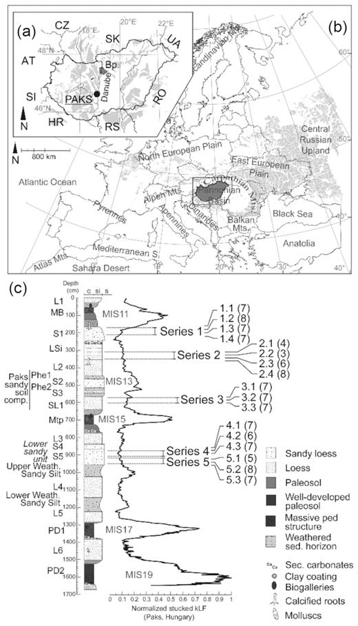
The locality of the Paks profile in (a) Hungary and in (b) the European Loess Belt (the European loess map is based on Haase et al.2007). AT, Austria; CZ, Czech Republic; HR, Croatia; RO, Romania; RS, Republic of Serbia; SI, Slovenia; SK, Slovak Republic; and UA, Ukraine. (c) The stratigraphic position of the sampled palaeosol horizons, the suggested series (1 to 5) and the members of the series (see more information in Section 2). The numbers in brackets indicate the number of samples taken from the same horizon for AMS measurements. For more information about the recent chronostratigraphic subdivision of the site, please see Újvári et al. (2014). The figure is a modified version of the figure published in Bradák et al. (2018a). MB, Mende Base soil; Mtp, ‘forest soil’; PD1, PD2, Paks Double palaeosol complex; L1–L6, loess; SL1, sandy loess; S1–S5 (fine), sand; Lsi, laminated silt; c, si, s, clay, silt and sand.
Thus, in the MF, formed of elongated magnetic minerals, the orientation of the long axis is determined by the maximum principal susceptibility (κmax), and that of the shortest axis by the minimum principal susceptibility (κmin). Theoretically, if the dust was deposited on a nearly horizontal surface the bedding-dominated fabric would be defined by κmin, its orientation being the bedding pole. The κmax and intermediate susceptibility axes (κint) will lie on the bedding plane, with the orientation of κmax indicating the palaeowind direction. This type of magnetic fabric is called ‘flow-aligned fabric’, in which elongated grains tend to align parallel to the direction of transport, and may thus indicate an up-flow tilting (i.e. imbrication; e.g. Thistlewood & Sun 1991; Nawrocki et al.2006). This MF type is frequently used during the reconstruction of Quaternary palaeowind direction in loess ( Thistlewood & Sun 1991; Lagroix & Banerjee 2002, 2004a; Zhu et al.2004; Bradák 2009; Zhang et al.2010; Liu & Sun 2012). The described MF type is the most common, regular in loess.
An MF, characterized by low-field anisotropy of magnetic susceptibility (AMS) measurements, reflects not only the alignment of the mentioned high saturation magnetization minerals, which have pdo-determined magnetic anisotropies, but that of other minerals that have crystallographic preferred orientation (cpo)-controlled magnetic anisotropies (Tarling & Hrouda 1993). Recent studies of various materials, including loess, have already demonstrated that the crystallographic anisotropy of various materials may influence the MF. Indeed, some observations (e.g. Rochette 1987; Hrouda & Jelinek 1990) suggest that the MF of materials with low-field magnetic susceptibilities (κlfavg < 5 × 10⁻⁴ SI) can be influenced by paramagnetic components.
Along with crystallographic bias, various processes can also disturb the sedimentary MF of loess and create an ‘irregular’, that is a non-flow-oriented, MF in loess. Increasing the energy of transportation can cause the rolling and traction of the clasts. As a result of rolling, the long axes of clasts tend to be aligned perpendicular to the flow direction, and the intermediate axes in the direction of flow in the so-called biaxial (prolate) orientation (shear stress related; e.g. Lagroix & Banerjee 2004b), flow-transverse fabric (sedimentary process related; e.g. Bradák et al.2018a) and L-tectonite type MFs (Borradaile 2001). This is also referred to as ‘AB plane imbricated fabric’ and ‘pencil fabric’ (e.g. Bradák et al.2011; Bradák-Hayashi et al.2016). Two different types of sedimentary flow-transverse fabrics are described in the literature by the alignment of principal susceptibilities on stereoplots: (i) the orientations of principal susceptibilities are well separated, and the current orientation is indicated by a 10–20° dip in κmin and the orientation of κint; (ii) the other is characterized by well-clustered κmax directions, while κmin and κint are intermixed along an axis on the foliation plane. In both types, the transport direction is perpendicular to the orientation of κmax. Similar fabrics are reported from Alaskan loess and are interpreted to be the result of shear stress (Lagroix & Banerjee 2004b), but in general flow-transverse fabrics are uncommon in loess (e.g. Zeeden et al.2015). Along with the shear stress–related origin of this fabric type, generally the appearance of this irregular MF can be interpreted as being the result of increasing energy of transport in the aeolian (Bradák et al.2018a) and/or water-lain depositional environment (Bradák et al.2011; Bradák-Hayashi et al.2016).
‘Disturbed’ or altered MFs readily develop during and after the diagenesis of loess under various conditions, such as deposition on a slope, in local depressions, in a permafrost environment, under erosion and redeposition by run-off water, and in the course of pedogenesis (e.g. Lagroix & Banerjee 2004a; Bradák et al.2011; Bradák & Kovács 2014; Ge et al.2014; Taylor & Lagroix 2015; Bradák-Hayashi et al.2016). If dust was deposited on a slope, the dip direction can be identified by the principal susceptibilities: the tilt of κmin directions from the vertical and the inclination of the plane defined by the alignment of the κmax and κint (Rees 1966; Bradák et al.2011; Ge et al.2014). The deviation of κmin from the vertical has been interpreted as cryptic post-depositional deformation/reworking in the course of permafrost processes (Lagroix & Banerjee 2004a; Taylor & Lagroix 2015). The deviation of the κmin inclination from the vertical, along with the chaotic alignment of the principal susceptibilities and isotropic MF, may be the result of pedogenesis (Matasova et al.2001; Hus 2003). An inverse magnetic fabric is also a possible marker of pedogenesis, indicating the vertical orientation of the elongated grains (pdo). An inverse MF may develop under the influence of vertical processes in palaeosols (Matasova & Kazansky 2004; Bradák et al.2011; Bradák-Hayashi et al.2016) and might also be the result of stable single-domain (SSD) magnetite (Hrouda 1982) and by the cpo of minerals such as siderite (Hrouda 1982; Rochette 1988; Márton et al.2010). Inverse MF is rare in loess, and has so far been identified in only a few loess profiles (e.g. Bradák et al.2011; Bradák-Hayashi et al.2016).
The goal of this study is to uncover the possible origin of the unusual MFs, found in Paks loess, and their potential significance in palaeoenvironment reconstruction.
2 MATERIALS AND METHODS
2.1 Materials
The Paks loess profile is located north of the town Paks in the Pannonian Basin, Hungary, on the right bank of the River Danube. A 16-m-thick loess/palaeosol sequence was investigated in a brickyard (Fig. 1). In this study, the aim is to introduce some unusual MFs found during the AMS study of the profile, and so no detailed lithostratigraphical description is presented here; one may, however, be found in Bradák et al. (2018a).
Oriented block samples of about 10 × 10 × 10 cm were collected at 10 cm intervals. Cubic specimens of 2 × 2 × 2 cm were cut from the block samples. No plastic holder was employed in order to avoid fabric deformation during sampling.
In the course of the AMS measurements (Bradák et al.2018a,b) what in this study are referred to as ‘irregular MFs’ were identified in stereoplots originating from five units of the succession (Fig. 1); these irregular MFs are unusual in loess profiles, and as mentioned above, may be related to pedogenesis, seismic/tectonic activity, permafrost and sedimentary processes (Section 1).
As previously indicated, one type of MF can be related to various processes. Instead of the study of just the irregular fabric, the MFs of the over- and underlying units of the layer with irregular MF were analysed together (Series 1 to 5; Fig. 1b) to narrow the range of possible forming processes down and determine the most appropriate one. This ‘combination or series’ of various types of MFs (introduced in Section 1) is characteristic of various processes of formation which can be revealed by AMS. The main characteristics of the sediments, where the studied sample series are originated from, are the following.
Series 1 contains four members (1.1, 1.2, 1.3 and 1.4). The studied material is the underlying poorly sorted greyish-orange sandy loess of the Mende Base (MB) palaeosol (Bradák et al.2018b), with a loose, homogeneous sedimentary structure, and on a scale of millimetres, carbonate concretion and manganese dots. Based on stratigraphical correlation (Újvári et al.2014), the studied material may be dated to MIS12 and/or MIS11.
Series 2 contains four members (2.1, 2.2, 2.3 and 2.4; Fig. 1). The unit is a well-sorted, grey, thinly laminated silt with a parallel wavy structure and secondary carbonate present between the sediment laminas. No deformation-related sedimentary structures were identified in the unit. The material was possibly deposited by water-lain processes in the course of, and interrupting an episode of, loess deposition. The chronostratigraphical position of the unit remains as yet unclear, though it may possibly date back to an early period of MIS12, at least as far as stratigraphical correlations might lead us to believe (Újvári et al.2014).
Series 3 contains three members (3.1, 3.2 and 3.3; Fig. 1). The material of the series is a yellow, homogeneous, well-sorted fine sand without any sedimentary structure. The fine sand unit consists, in turn, of a darker weathered horizon, possibly part of the weak MIS13 (Paks sandy soil complex; Újvári et al.2014) palaeosol complex. The sandy silt horizons could be deposited during a cooler stadial period or at the end of MIS14 glacial. On the basis of stratigraphical correlation, the unit may be dated to the MIS 13 or late MIS14.
Series 4 (4.1, 4.2, and 4.3) and 5 (5.1, 5.2 and 5.3) originate from the same sediment layer (Fig. 1). The material of the series is greyish–redish yellow, loose fine sand/sandy loess with a parallel wavy, rhythmic lamination, silt and fine sand laminae alternating. No deformation of the sedimentary structure was identified in the layer. On the basis of its stratigraphical position, the unit may be dated to MIS16 (Újvári et al.2014).
2.2 Methods
To estimate magnetic carriers and their domain state, hysteresis measurements were conducted using a Micromag 3900 alternating gradient magnetometer (Princeton Measurements Co.).
Hysteresis curves show the induced magnetization of a sample as a function of an applied field with up to 1T field strength (high field; e.g. Tauxe et al.1996, 2010; Roberts et al.2017).
Temperature variation in magnetic susceptibility (kT) was measured using an MFK1-FA Kappabridge susceptibility meter coupled with a CS-4 furnace apparatus for high-temperature susceptibility measurements ‘in air’ (AGICO, Czech Republic). kT were measured at temperatures of up to 700 °C and measurements were taken quasi-continuously.
The frequency dependence of magnetic susceptibility is a good tool to determine the amount of superparamagnetic (SP), pedogenic contributors in the samples (Forster et al.1994). It was measured by the SM-100 ZH-Instrument (low frequency 0.5 kHZ and high frequency 4 kHz). For SM100 the sensitivity is ∼5 × 10⁻⁶ SI units at 0.5 kHz; therefore, the bias of the results cannot be excluded during the measurement of samples with low magnetic susceptibility. The relative frequency dependence of magnetic susceptibility (|$\chi$|fd per cent) is the rate of the magnetic susceptibility of the sample measured at low (χlf) and high (χhf) frequencies: χfd per cent = (χlf− χhf)/χlf × 100. And it was used to identify the increasing relative amount of in situ–formed SP minerals, which may indicate pedogenic processes.
Low-field volumetric magnetic susceptibility (κlf) and MF were investigated using 111 cubic samples; in general, 6–10 samples were collected from each 10-cm sediment interval. AMS parameters were determined by measuring a specimen in 15 positions using a KLY-3S Kappabridge (AGICO) instrument. The intensities and directions of principal susceptibilities (κmax, κint, κmin) were determined by computer analysis, and numerous statistical parameters were calculated and used to characterize the MF calculated using the principal susceptibility values (Anisoft 4.2 software). In the course of data verification, results with negative F statistics (F < 3.48; 95 per cent significance level; Jelinek 1977) were excluded. Various AMS parameters were also examined, following the method of Lagroix & Banerjee (2004a) and Zhu et al. (2004). The F12–ε12 plot was studied to identify significant lineation in the samples (Zhu et al.2004). Furthermore, the relationship between foliation and F23 was also investigated (Zhu et al.2004) in order to reveal well-resolved magnetic foliation in the fabric (F23 > 10). The analyses also included the investigation of F12 and volumetric susceptibility relations to identify random measurement error in samples (Zhu et al.2004). Where the F12 and ε12 statistics did not show strong anisotropy, but the alignment of the principal susceptibilities, related to the same stratigraphic horizons, indicated some characteristic orientation or fabric in the stereoplots, the data from those samples were used (see the Supporting Information).
Basic anisotropy parameters, such as lineation (L) and foliation (F), were calculated as L = κmax/κint and F = κint/κmin (Hrouda 1982). The corrected degree of anisotropy was calculated as in Jelinek (1981).
The relationship between the shape of the susceptibility ellipsoid (T) and the degree of anisotropy (P) was characterized by a Jelinek diagram (Jelinek 1981).
Five or more samples/horizons are needed to provide a statistically significant data set during the stereoplot analysis. During the sample preparation, some samples were lost; therefore, in the case of Series 2 (2.1 and 2.2 subunit) only four and three samples were analysed. Less than five samples can provide information about the AMS parameters, but limited information about the alignment of the axis of the principal susceptibilities. The alignment of the principal susceptibilities was plotted and analysed on stereoplots using an equal-area projection and geographical coordinate system.
Box-and-whisker plots may be used to visualize more than one statistical parameter, so this method was applied to characterize some basic parameters of the studied series. The boxes denote the interquartile range, whereas data falling within 1.5 times the value of the interquartile range are represented by the two T-bars (the lower and upper whiskers). Circles indicate outliers (data between 1.5× and 3× the interquartile range), while asterisks mark the extreme outliers (values 3× higher than the interquartile range). The black line within the box shows the median (Norušis 1993; Bradák & Kovács 2014).
As an experiment, the AMS parameters of the samples from each studied series (Series 1 to 5; see above) were reclassified and artificial sample groups were created. As a conceptual idea, these artificial groups would represent characteristic magnetic fabrics and help to reveal the relationship between the forming of the original series.
An eigenvector equation yields the solution, and furthermore, the vectors can be sorted according to the degree of importance given to them by the corresponding eigenvalues. In this way, the first two vectors may be used to visualize the separation of the groups, achieved by plotting |$L{D_1}$| = X|${a_1}$| against |$L{D_2}$| = X|${a_2}$|, where X denotes the (|$n \times p$|) data matrix with all n observations from the p measured parameters. Additionally, linear discriminant functions may be defined using the previously obtained vectors |${a_i}$| so that observations may be classified into one of the k groups. If the discriminant functions are used as a decision rule, the class membership of the original observations may be predicted. Seeing as the correct original underlying classes of these cases are already known, a percentage of cases correctly classified by LDA is obtained. If the labels were in the first instance derived with the use of a clustering algorithm, the quality of the obtained grouping may also be evaluated by examining the percentage of cases classified correctly by LDA (Kovács et al.2012).
In this equation, the superscript l indicates the ith parameter. |${x_{ij}}^l$| is the jth member of the ith group (for the lth parameter), |${{\bar{x}}_{i}}^l$| is the mean of the i group, and |${{\bar{x}}^l}$| is the total mean for all observations for the lth parameter. The resulting Wilks’ λ is a number between 0 and 1; and if Wilks’ λ for the lth parameter is 1, there is no inter-group variability, that is, that particular parameter does not affect the classification, while if the value is 0, the parameter under consideration has the greatest degree of influence on the obtained classification.
During the re-classification, the AMS parameters of the original samples were used, thus each mathematically created group represents a different MF type with its own characteristic distribution of F, L, P and T values.
The samples from each mathematically (artificially) created group were plot on Jelinek diagram (P–T diagram). Based on the distribution of the samples of each group, various provinces were separated in the plot, which indicates characteristic MF types based on the LDA analysis of the AMS parameters of the studied series (Series 1 to 5). The average values of the samples from the members of each series (i.e. the original Series 1 to 5) were re-plotted in the new Jelinek diagram (see below in Section 3.2). The described method of sample analysis has three elements: (1) re-classification of the samples (the creation of artificial sample groups by LDA based on AMS parameters), verification of the artificial groups and revelation of the mathematical similarities by LDA; (2) the determination of MF provinces on a new Jelinek plot; and (3) the allocation of the average values of the samples from the original series on the new Jelinek plot. These three elements assist the researcher in finding similarities and differences between the origin and forming processes of the members of the original series.
3 RESULTS
3.1 Rock magnetism
The hysteresis loop of the pilot samples showed the characteristics of so-called pseudo-single-domain (PSD; mixture of single domain, SD, and multidomain, MD, or single vortex state; Tauxe et al.1996, 2010; Roberts et al.2017) magnetic grains in the studied samples (Figs 2a–h). All of the hysteresis loops are narrow (indicating a relatively small coercive force), and the ferromagnetic components, indicated by the corrected hysteresis curves, are saturated in a low level of applied field (∼200–300 mT; Figs 2b, d, f and h). Above this level, the induced magnetization of the samples is constant in the corrected curves, but it increases quasi-linearly in the non-corrected curve. In the non-corrected curves, a linear increase in magnetization is to be observed with an increasing magnetic field and this feature can be connected to, for example, high-saturation components (e.g. hematite and/or goethite) and paramagnetic contributors (Richter & van der Pluijm 1994). In the case of the studied series, this phenomenon indicates 66 per cent paramagnetic (and high coercivity) components in 1.4, 58 per cent in 2.3 and 3.2, and 44 per cent in 4.2, respectively.
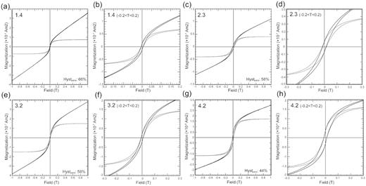
Results of the hysteresis experiments. The hysteresis curve of 1.4 (a, b), 2.3 (c, d), 3.2 (e, f) and 4.2 (g, h) members of the series.
A typical thermal change in magnetic susceptibility is shown in Fig. 3. A gentle peak or ‘hump’ may be observed at around 125 and 150 °C in the heating curve of samples 2.3, 3.2, 4.2 (Figs 3a, c and d). A similar hump is also seen at around 200 and 250 °C in samples 2.3 and 5.2. Most of the heating curves display a decreasing value of susceptibility at around 300 °C, followed by an increase between 320 and 400 °C (Fig. 3a). This phenomenon is very characteristic in the kT curve of 2.3 (Figs 3a and c). Above that, most of the heating curves show a linear decrease with steps e.g. at 450 °C (samples 2.3 and 4.2; Figs 3a and c) and 530 °C (2.3, 3.2, 5.2; Figs 3a and c) up to about 570 °C, followed by a sharp drop at 580 °C, the Curie temperature of magnetite, and a peak and then a gradual decrease to zero at about 680 °C, the Curie temperature of haematite (Figs 3a, c and d), with the exception of sample 1.4, in which no peak could be identified. During cooling, susceptibility recovered rapidly, at 400–500 °C in sample 3.2 (Fig. 3d), gradually with steps in samples 2.3, 4.2 and 5.2 (Fig. 3c), and gradually, similar to the heating curve in sample 1.4, until 50 °C (Fig. 3b).
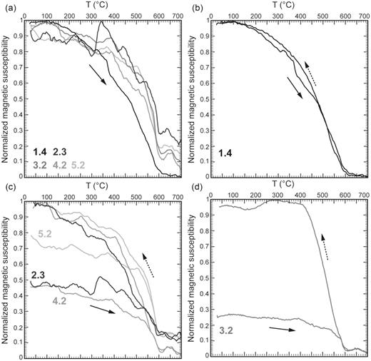
Temperature variation in magnetic susceptibility (kT plot). All of the normalized heating kT curves (a), and separately by their characteristics during heating and cooling: no characteristic change in susceptibility during cooling (b), moderate increase of the cooling susceptibility compared to the heating curve (c) and rapid increase of susceptibility during cooling (d).
The highest □fd per cent (SP contribution) was notified in the samples from Series 1 (∼10–14 per cent). Series 3, 4 and 5 are characterized by lower, ∼6–10 per cent SP components. The lowest □fd per cent, 2–8 per cent, was revealed in the samples of Series 2 (see the Supporting Information).
3.2 Magnetic fabric parameters
The basic MF characteristics (κlf, P and T) of the studied series were described using box–whisker plot analysis (Fig. 4). All of the samples in the series are characterized by a low κlf. It should be noted that the range of κlf values of Series 2, 3, 4 and 5 is lower, narrower and more well-defined than that of the κlf of Series 1 (Fig. 4a). This is characterized by slightly higher and more scattered values (Fig. 4a). Two types of P distribution of samples were revealed by the analysis (Fig. 4b). Series 1 and 2 samples were characterized by a narrow range of P, while Series 4 and 5 values were distributed over a wider band. Series 3 was characterized by a slightly wider range of P than Series 1 and 2 (Fig. 4b). All of the T distributions of the series were scattered and contain negative values, indicating the appearance of lineation and prolate MF (Fig. 4c). An exception is Series 2, in which the distribution of T is narrow and most of the samples were characterized by moderate/strong oblate (foliated) MF (T > 0.5).
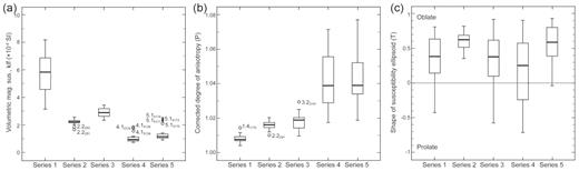
Broad characterization of the κlf (a), P (b) and T (c) distribution in the studied series. The interquartile ranges are represented by the lower and upper whiskers (T-bars). Circles indicate outliers and asterisks mark the extreme outliers. The black line within the box indicates the median value.
The significance of lineation and foliation of individual specimens was tested and characterized in numerous ways (Fig. 5) The ε12–F12 plot reveals a significant lineation (F12 > 4) for most of the Series 1 and 2 samples and a weak and non-lineated fabric is observed for Series 3, 4 and 5 (Figs 5a and b). The plot of all data L–ε12 indicates a moderate/weak inverse relationship (exponential trend, R2: 0.28), while the L–ε12 plots with the series displayed separately show a stronger linear relationship (R2: 0.4–0.58, respectively; Fig. 5b). As an exception, a weak correlation is observed for the plot with only Series 2 data (R2: 0.19). No significant relationship is observed between the bulk susceptibility and F12 (Fig. 5c). Most of the samples from various series are characterized by values of F23 > 10 in the plot F–F23 (Fig. 5d).
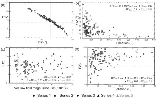
Data verification and characterization of the foliation and lineation in the MF by (a) a ε12–F12 plot, (b) an L–ε12 plot, (c) κlf–F12 plots and (d) F–F23. The symbols are 50 per cent transparent to show the overlapping of the members from various series.
A Jelinek diagram was employed to reveal the ‘in-series’ differences between the members (Fig. 6). The members of Series 1 were characterized by the lowest P among the studied series (PAVG: 1.007–1.009) and by the scattering of T between the strongly oblate and prolate MFs (TAVG: −0.43 to 0.81; Fig. 6a). Compared to other series, the P and T values of Series 2 were less scattered, and there are no significant differences between the P (1.012–1.019) and T (0.51–0.65) values of the members (Fig. 6a). The P and T distribution of Series 3 was similar to that of Series 1 with slightly higher and more scattered P (PAVG: 1.016–1.019; TAVG: 0.11–0.41). The P of Series 4 (PAVG: 1.027–1.051) and Series 5 (PAVG: 1.037–1.045) were similar and the highest among the studied series (Fig. 6c). Of the two series, the members of Series 4 were characterized by lower T, oblate and prolate susceptibility ellipsoid (TAVG: −0.24 to 0.37) than those of Series 5 (TAVG: 0.46–0.8), indicating a mainly moderate/strongly oblate, foliated MF (Figs 6d and e).
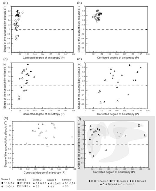
The distribution of the AMS parameters on the Jelinek diagram. The various grey tones of the symbols indicate different members of Series 1 (a), Series 2 (b), Series 3 (c), Series 4 (d) and Series 5 (e), respectively. (f) The distribution of the samples of the reclassified groups and the average group statistics (P and T) of the original members of Series 1 to 5, respectively (grey background area). The reclassification of the samples is based on LDA. During the reclassification, AMS parameters were used; thus, each group represents a different MF type with a characteristic P and T distribution. The polygons (Groups A, B, C, D and E) indicate the distribution of P and T values of the samples from each mathematically created group (for more information please see Sections 2.2 and 3.2).
Wilk's Lambda analysis was carried out on the original data set to reveal which AMS parameters are significantly different in and characteristic of each series (Series 1 to 5). The Wilk's Lamda analysis shows the importance of various AMS parameters in the differences in the series. Based on the Wilk's lambda, P (0.3), F (0.44) and L (0.55) were the most important AMS parameters (see the Supporting Information). The analysis showed that 63 per cent of the original grouped cases were correctly classified, meaning that 63 per cent of the samples are similar to the other members of the studied series, on the basis of mathematical analysis. It also demonstrates the possibility of overlapping between the characteristics of the magnetic fabric of the series. Although there are differences between the sedimentary character of the studied series (Series 1 to 5), the mathematical analysis suggests some similarities and an overlapping in AMS parameters, possibly indicating a similar origin for the MF (Section 4.2).
3.3 The reclassification of the samples and the AMS characteristics of the artificial sample groups
Along with the characterization of the series, artificial groups of samples were created through the reclassification of the samples by LDA based on their AMS parameters (Section 2.2).
The P and T of the samples of various artificial groups were plotted on a new Jelinek diagram (Fig. 6f). The samples from five groups were located in various parts of the plot. Samples from Groups A and B were located in moderate and weak, oblate and prolate (0.6 > T > −0.4) susceptibility ellipsoid area, with weak anisotropy (P < 1.02; Fig. 6f). Samples from Group C were located in the area of the strongly oblate (T > 0.6) susceptibility ellipsoid but relative weak anisotropy (P < 1.02; Fig. 6f). Samples from Group D were located in the strong and moderate oblate (1.0 > T > 0.2) susceptibility ellipsoid area, with stronger anisotropy (P > 1.03; Fig. 8). And samples from Group E were located in the strong oblate to strong prolate (0.8 > T > −0.8) susceptibility ellipsoid area, with stronger anisotropy (P > 1.02; Fig. 6f).
The average T and P values of the members of the original series were added to the plot to reveal any possible similarities and differences in the MF of the studied series. Series 1 and 3 members fell within the area of Groups A and B defined by scattering T between the oblate and prolate fabric and weak anisotropy (Fig. 6f). The average T and P of the members from Series 2 were located on the borderline of the area of Group C defined by strong oblate and weak anisotropy (Fig. 6f). The average T and P of the members of Series 4 and 5 were settled in the overlapping area of the locations of Groups D and E, with stronger anisotropy and various T (Fig. 6f).
3.4 Stereoplot analysis
Stereoplot analysis was applied to reveal the alignment of the magnetic grains in the fabric. Most of the under- and overlying members of the studied series were characterized by quasi-horizontal foliation occasionally with a dip of a few degrees, indicated by the ∼90° inclination of κmin (1.1 and 1.2 in Fig. 7a; 2.1 in Fig. 7b; and 4.1 in Fig. 7d), and its discrepancy of a few degrees from the vertical (5–15°) in some cases (3.1 and 3.3 in Fig. 7c and 5.3 in Fig. 7d). The kmax and kint principal susceptibilities are poorly to well aligned on a quasi-horizontal plane.
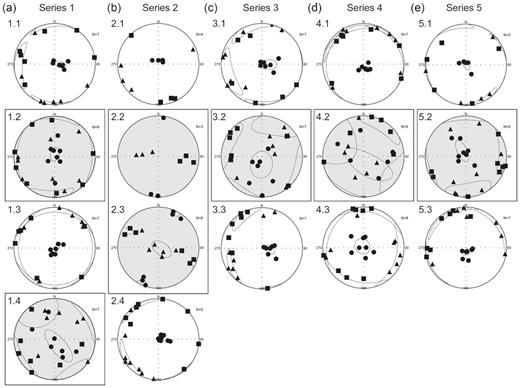
Unusual magnetic fabric of some units from Paks. Series 1 to 5 (letters ‘a’ to ‘e’) represent various parts of the studied succession (for a detailed description of the sampled units, please see Section 2.1) and contain three or four members, marked by 1.1, 1.2, 1.3 … 5.3. The first number indicates the series, where the studied member belongs, and the second number marks its position in the series, counted by the top. Members with an unusual MF were marked by grey colour. The principal susceptibilities are plotted in equal area projection, geographical coordinate system, and marked by ▓ maximum susceptibility, ▲ intermediate susceptibility, and ● minimum susceptibility. The alignment and scattering of the principal susceptibilities are represented by 95 per cent confidence ellipsoids.
In the MF of samples 3.2, 4.2 and 5.2, the κmax is moderate/well clustered and κmin and κint are intermixed along an axis on the foliation plane (Figs 7c–e). The alignment of the principal susceptibilities followed a similar but poorly aligned and difficult to define pattern in the MF of samples 1.2 and 1.4 (Fig. 7a). In the MF of 2.3, κmin directions are well clustered and κmax and κint are settled, slightly intermixed along an axis, on the foliation plane (Fig. 7b).
4 DISCUSSION
4.1 Rock magnetic components of the series
Based on the rock magnetic experiments, various types of ferromagnetic minerals with a mixture of SD and MD magnetic grain sizes contribute to the magnetic fabric of the samples, along with a significant amount of paramagnetic components in the fabric of 1.4, 2.3 and 3.2.
The gentle peak in samples 2.3, 3.2, 4.2 at around 125–150 °C (Figs 3a, c and d) suggests the transformation of goethite (αFeOOH), at 120 ± 2 °C (Özdemir & Dunlop 1996; Fig. 3). The slight increase in susceptibility about 200 °C likely reflected the unblocking of SD particles (Liu et al.2005), which suggests that those samples contain ultrafine pedogenic ferrimagnetic grains of a size near the SD/SP boundary (2.3 and 5.2; Fig. 3c). There was also a slight decrease in susceptibility at 250–320 °C, followed by a rapid increase at 320–330 °C (2.3 and 5.2; Figs 3a and c), which probably represented the neoformation of magnetite, likely from the decomposition of maghaemite into magnetite (Liu et al.2010; Liu et al.2013) or, alternatively, the alteration of maghaemite to haematite (Sun et al.1995). Step-like decreases at various temperatures, for example 400–450 °C (samples 2.3 and 4.2) and 530 °C (2.3, 3.2 and 5.2), could be due to titanomagnetite/titanomaghaemite with various Ti contents (e.g. Deng et al.2000; Lattard et al.2006; Figs 3a and c). The presence of ilmenite/titanomagnetite was also supported by the SEM study in both sediment and palaeosol samples (Bradák et al.2018a). The decrease in magnetic susceptibility at 580 °C shows that magnetite grains were also present. This decrease was followed by a further gradual decrease followed by a gentle peak to about 680 °C, the Curie temperature of haematite. The peak observed in all samples except 1.4, with a local maximum around 660–680° C, may be identified as a Hopkinson peak (Figs 3a, c and d), a characteristic mark of haematite at around its Curie temperature. Although the appearance of high-coercivity magnetic components, most likely haematite, was already verified by isothermal remanent magnetization experiments in Hungarian loess (including Paks; e.g. Bradák et al.2011, 2018a), the formation of haematite by the oxidation of maghaemite during the in-air experiments cannot be excluded.
In sample 3.2, the recovered magnetic susceptibility was much higher than the original susceptibility, and significantly higher in samples 2.3, 4.2 and 5.2, also. This phenomenon may possibly be related to the neoformation of magnetite (or maghaemite) from clay minerals during the heating treatment (e.g. Ao et al.2009; Figs 3c and d).
We cannot exclude the possibility of the influence of paramagnetic contributors to the susceptibility signal of samples characterized by a magnetic susceptibility of κlf < 5 × 10⁻⁴ SI (e.g. Hrouda & Jelinek 1990). The contributions of paramagnetic components were roughly estimated by the hysteresis curves (Fig. 2; Richter & van der Pluijm 1994). In summary, possible contributors to the magnetic fabric include the mixture of SD and MD magnetite, titanomagnetite, ilmenite, maghaemite, haematite and paramagnetic grains such as muscovite, biotite and chlorite. The appearance of the suggested contributors is supported by the results of the SEM observation presented in Bradák et al. (2018a,b).
4.2 Differences and similarities in the MF of the series
The AMS experiments revealed that the most common among the studied MFs is the flow-oriented fabric. All the over- or underlying units of horizons with irregular fabric in the series were characterized by a flow-oriented fabric (Fig. 7), except the MF of unit 5.1, identified in Series 5 where gravitation dominated during the sedimentation (Fig. 7e). The MF of 5.1 displays a quasi-horizontal foliation with a dip of a few degrees and scattered alignment of the elongated grains over a horizontal plane, without any characteristic fabric lineation.
There are two characteristic depositional environments of loess in which the mentioned regular MFs were formed. In the first type of environment, through the development of non-flow-aligned (poorly lineated, mainly foliated) fabric, the gravitational force dominates over the tangential force (stereoplots 1.1 and 5.1; Figs 7a and e). The theory of a poorly lineated, mainly foliated loess is supported by studies conducted by Hus (2003), who observed that the gravitational force and compaction play leading roles in the development of the MF of loess. In the second type of environment, where the most common flow-aligned loess MF developed, the elongated grains tend to align parallel to the direction of transport and usually display an up-flow tilting (imbrication; Figs 7a–e, except stereoplot 1.1, 5.1 and the marked irregular samples). The imbrication can be observed in the 5–20° dip of the MF to the horizontal plane of foliation (a deviation of κmin from the vertical; e.g. Nawrocki et al.2006). As already mentioned, the flow-aligned MF type is the most common in loess deposits and is reported in numerous studies, such as that of Thistlewood & Sun (1991), Begét et al. (1999), Lagroix & Banerjee (2002), Zhu et al. (2004, 2004a), Bradák (2009), Zhang et al. (2010) and Liu & Sun (2012).
Irregular MFs are defined as those with a biaxial prolate orientation/flow-transverse/or L-tectonite fabric (stereoplot 1.2, 1.4, 2.2, 2.3, 3.2, 4.2 and 5.2; Fig. 7). Along with these, a unique, new loess MF was identified in Series 2 (stereoplot 2.3; Figs 7b and 8a) by comparing the characteristics of the irregular MF to each other.
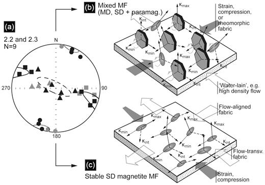
The interpretation of the alignment of magnetic minerals and some theories about the origin of the unique MF found in 2.3 of Series 2. The principal susceptibilities are ploted in equal area projection (a), a geographical coordinate system, and marked by ▓ maximum susceptibility, ▲ intermediate susceptibility and ● minimum susceptibility (grey coloured—2.2; black coloured—2.3). The alignment and scattering of the principal susceptibilities are represented by 95 per cent confidence ellipsoids.The grey-coloured elongated-shape grains represent the MD, SD and SP ferromagnetic components, such as magnetite. The grey-coloured polygons represent paramagnetic contributors, such as biotite. The small arrows indicate the orientation of the principal susceptibility axis: solid line—κmax; dashed line—κint; dotted line—κmin. The white, wide and transparent arrows indicate sedimentary processes, the direction of the palaeocurrent (windt or water-lain processes). The dark grey, wide and transparent arrows indicate strain, compression, triggered by mass movements (e.g. creeping) or seismic activity. The light grey arrows indicate rolling grains during the transportation by the palaeocurrent.
In the irregular MF of 2.3, characterized by well-clustered kmin directions, kmax and kint are mixed along an axis on the foliation plane (Fig. 8a). This type of MF had not been previously observed in loess, and there some hypothesis about the interpretation of the results and the forming of such fabric:
The alignment of the principal susceptibilities possibly indicates the appearance of the mixture of rotated elongated minerals (along the shortest axis; e.g. magnetite) and vertically oriented (platy) minerals (e.g. phyllosilicates; Fig. 8b) and interference with the ferromagnetic fabric by paramagnetic components. In materials with low κlf (κlf < 5 × 10⁻⁴ SI; Figs 1 and 4), such as the Series 2 samples (∼2.2–2.3 × 10⁻⁴ SI), interference with the ferromagnetic fabric by the paramagnetic components has been suggested by Rochette (1987), Hrouda & Jelinek (1990) and Hrouda et al. (1997). Previous SEM observations also revealed a significant amount of paramagnetic components (especially but not limited to phyllosilicates) compared to the amount of ferromagnetic contributors in Paks loess (Bradák et al.2018a,b). In the fabric containing phyllosilicates, the well-aligned κmin directions are subparallel to the crystallographic c-axis and perpendicular to the depositional plane (Biedermann et al.2014). Compared to κmin, the κmax and κint axes are randomly or poorly aligned. In the case of 2.3, the mixing of κmax and κint possibly indicates the rotated orientation of elongated, high saturation magnetization minerals and the vertical orientation of the two longer crystallographic axes of phyllosilicates, such as muscovite and/or biotite, which are possibly oriented by some kind of sin- or post-depositional horizontal strain, for example compression (Fig. 8b).
Due to the sedimentary character of the studied material (Section 2.1), which indicates water-lain processes, the redeposition of the material as water-lain redeposition or water-saturated high-density flow can be also assumed. Unfortunately, the MFs of water-lain redeposition or high-density materials are flow-oriented, flow-transverse or chaotic (e.g. Taira 1989; Bradák et al.2011; Tamaki et al.2015) and therefore the observation of high-density sediments (e.g. turbidite) does not support the idea.
As it was suggested above, the lamination of the unit possibly indicates water-lain primer processes, which are generally characterized by a quasi-horizontally foliated fabric (with a flow-oriented or flow-transverse MF). The irregular fabric may form by water saturation and the later-stage deformation of primer foliated fabric possibly associated with the slow emplacement of the material (slope processes, e.g. creeping). A similar deformed, but not tectonized, so-called rheomorphic MF was introduced by Tarling & Hrouda (1993).
Interpreted differently, the MF of 2.3 can be interpreted as an MF composed of predominantly ultrafine (stable single domain—SSD) magnetite grains that are lying on the quasi-horizontal sedimentation plane (Fig. 8c). The κmax of SSD magnetite indicates the short crystallographic axis, and the κmin indicates the orientation of the longest crystallographic axis (Hrouda 1982). Thus, the observed alignment can be described as an MF made of elongated-shape ultrafine SSD minerals, which aligned perpendicular to or parallel to the current on a horizontal depositional plane (Fig. 8c). It can be interpreted as an MF possibly oriented by some kind of sin- or post-depositional horizontal strain, for example compression (Fig. 2c). The mixed mineral composition of 2.3 (see above, in the rock magnetic results) does not support the idea of an exclusively ultrafine SSD MF.
During the classification of the irregular fabrics, three different types of series can be recognized in the five MF series based on the stereoplot analysis (Fig. 7), the relationship of the AMS parameters (Figs 5 and 6) and the reclassification of the samples (Fig. 6f).
The unique irregular MF of Series 2 is defined as being of the first type. There was no significant change in the P and T of the members of the MF of Series 2 (Figs 4b, c and 6b). Both the under- and overlying units and the 2.2–2.3 horizon were characterized by weak anisotropy (PAVG: 1.012–1019) and strong oblate, disc-shaped susceptibility ellipsoids (TAVG: 0.51–0.65). The similarity in the AMS parameters suggests that there was no significant change in the sedimentary environment. In contrast, the stereoplots clearly show the differences in the alignment of the principal susceptibilities, suggesting the influence of some (post)-sedimentary process, which was possibly able to realign the entire MF, including the ultrafine, coarse, ferro-, and paramagnetic components. Members of Series 2 originate from the same uniform sedimentary layers, and are characterized by very similar sedimentary and AMS parameters. Given this, a change in the sedimentary environment (e.g. catastrophic weather events that can be seen in the change of the sedimentary character also) can be excluded as a cause of the unusual MF. No marks of weathering or pedogenesis were identified in 2.3 by the field observation or, for example, by the increasing κlf and □fd per cent values (see the Supporting Information). For this reason, chemical alteration/pedogenic processes can also be excluded from the possible causes of its unusual MF. Tectonically triggered deformation is a possible candidate, as this might lead to the development of a similar, L-tectonite-type MF (Figs 7 and 8a; e.g. Borradaile 2001). The similarity in the orientation and the AMS parameters of the under- and overlying material of 2.3 possibly indicate that the environment ‘returned’ to its original (pre-event) condition after the supposed deformation. Seismic activity is one of the processes that may have caused soft sediment deformation in the unconsolidated material MF. The possible source of the seismic activity (palaeo-earthquakes) is a fault zone, identified in the neighbour of Paks (Tóth & Horváth 1999), and which is known to have been active in the Quaternary. Unfortunately, no marks of tectonic activity (e.g. faults) that might clearly demonstrate the validity, or not, of this hypothesis were detected in the profile. More (field) research is needed to verify the appearance of tectonic activity, for example by seismites in the surroundings of the Paks profile.
No characteristic change in P but a scattering T was observed in the MF of Series1 and 3 and was defined as the second type (Figs 4 and 6). A smaller, negative T of the samples indicates the change of the MF from a foliated, oblate to a prolate fabric with strengthening lineation. Despite the scattered T values, the P is quasi-constant. A constant P may well indicate a stable depositional environment, possibly forming the uniform MF in Series 1 and 3, while the unusual MF of 1.2, 1.4 and 3.2 was formed by the post-sedimentary alteration of the uniform MF (Fig. 7). Based on the marks of pedogenic processes, observed in the suggested horizons (e.g. darker colour, the presence of biogalleries; weak) pedogenesis may have been responsible for the formation of the irregular MF of Series 1 and 3. In the case of Series 1, the development of Mende Base palaeosol may have influenced the underlying horizon. In the case of Series 3, marks of weak pedogenesis were observed in the field in unit 3.2, possibly related to the formation of Phe1 or Phe2 sandy soil horizons (Section 2.1; Fig. 1). In contrast to the field observation (weak pedogenic character, bioturbation), no significant increasing □fd per cent can be observed in the sample; that is, the appearance of pedogenic processes is not supported by the magnetic measurements. It is possibly the result of very weak pedogenesis, and for example continuous sedimentation during the pedogenic phase, which did not allow the development of the soil (aggradation of the soil, when the rates of sedimentation and pedogenesis are in balance). The parallel appearance of continous sedimentation and weak pedogenesis with, for example, bioturbation (MF is similar to the disturbed MF in Bradák et al.2011) may describe the disturbed fabric and the dilution of the magnetic minerals (weak □fd per cent; see the Supporting Information).
The MFs of Series 4 and 5 samples were defined as of third type on the basis of their scattering and increasing P and T values (Figs 4, 6 and 7). Compared to the other series, the increasing P and the scattering values (Series 4—strengthening of L; and Series 5—weakening of F) possibly indicate a changing sedimentary environment in which the originally foliated MF (stereoplot 4.3 and 5.3; Figs 7a and e) weakened and reoriented by, for example, the increasing transportation energy (e.g. Bradák et al.2018a). The change in the depositional environment was not observable due to the uniform sedimentary character of the members of Series 4 and 5 in the field. By way of contrast, this may be recognized in the irregular MF of 4.2 and 5.2, which indicates rapid change by (1) the flow-oriented MF changing to a flow-transverse MF and back and (2) scattering AMS parameters (see above). The increasing energy of transportation/deposition did not cause significant change in the orientation; that is, the palaeocurrent orientation is N–NW, independent from the type of the MF (Fig. 7). The constant wind direction possibly indicates a longer and stable climatic period dominated by the same wind direction, which possibly represents the dominance of the same airmass over the region during the deposition of Series 4 and 5. These changes in the palaeoenvironment may be related to climate fluctuation or episodic, extreme weather events, such as cooler periods, with an increase in wind energy, dust/sand storms, and the redeposition of surface material during a stable longer glacial or stadial period with constant N/NW palaeocurrent (wind) direction.
5 CONCLUSION
Irregular magnetic fabrics were observed in the course of the low-field AMS investigation of a sedimentary record with various sedimentary characters in an Early Middle Pleistocene loess/palaeosol succession at Paks (Hungary). Although the materials indicate quasi-constant palaeoclimatological/palaeoenvironmental conditions over a longer geological period (e.g. a glacial in the Pleistocene), the characteristic change of the MF indicates short-term, possibly unusual event(s) during the (post-)sedimentation period. Three possible causes of the MF change and formation of the irregular MF have been suggested:
A swift, rapid change in the sedimentary environment which may be connected to abrupt climate fluctuation or extreme weather events.
Weathering and pedogenic processes, which may be responsible for the alteration of the MF during, for example, the warmer interglacials and interstadial periods of some glacial.
Meanwhile, non-palaeoclimate-related events, such as deformation processes triggered by earthquakes or palaeoseismic activity, can also overwrite the original sedimentary fabric, but more AMS study of seismic activity–related sedimentary features is needed to support this hypothesis.
Although some of the unusual MFs cannot be used for the determination of the palaeo-wind direction, the main goal of loess MF studies, this study has shown the significance of irregular fabrics in palaeoenvironmental reconstructions. The role of an unusual MF is recognized in its indication of non-linear climatic and tectonic events during the Quaternary, though its importance is not limited to this.
SUPPORTING INFORMATION
Supplementary Material 1. The AMS and rock magnetic parameters and the results of the LDA analysis, used in the study.
Suppl_mat_1online.pdf
Please note: Oxford University Press is not responsible for the content or functionality of any supporting materials supplied by the authors. Any queries (other than missing material) should be directed to the corresponding author for the paper.
ACKNOWLEDGEMENTS
We are thankful for the comments of the reviewers, Jerzy Nawrocki and an anonymous reviewer. A fellowship was awarded to BB at Kobe University, Japan, by the Japan Society for the Promotion of Science (JSPS) during the period of 2015.10–2017.10.
BB is grateful for the support and advice of Professor Masayuki Hyodo (Kobe University, Japan). We are also thankful for the rock magnetic experiments that were conducted at the Center for Advanced Marine Core Research, Kochi University.
Part of the research was supported by the Hungarian Scientific Research Fund (OTKA) K 119366.
